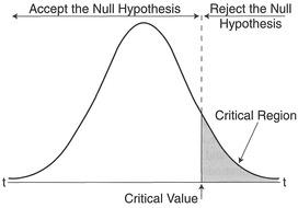
Figure 5.1 Rejection region for a probability distribution.
This chapter develops the themes discussed in Chapters 3 and 4 and is concerned with the formal statistical analysis of quantitative data, and the interpretation of results from such analysis. You should already be familiar with the process of setting up objectives or hypotheses, the construction of a sampling frame, the various types of data and the collection of data, as well as the pre-processing and the preliminary steps of data description which make up an Initial Data Analysis (IDA). Recall from Chapters 3 and 4 that these elements correspond to steps 1-4 of Chatfield's stages of a statistical investigation (see Box 5.1).
The remaining steps 5-7 are concerned with more formal statistical analysis procedures, the implications of a statistical investigation for placing the results in the wider context of established knowledge as well as in the more immediate context of the research project. It is step 5 which we shall examine in more detail in this chapter. Although elements of steps 6-7 are considered here, these elements are of more general application and are covered in more detail in Chapter 10.
It is not possible to cover in detail within the confines of one chapter all of the statistical methods of potential use to your research. We will restrict our
Box 5.1 Stages of a statistical investigation
Source: Adapted from Chatfield 1995.
focus to some of the techniques concerned with statistical inference and model construction which have been widely used by geographers. For further information on the methods described here, and additional methods which are not covered (e.g., multivariate methods), you should try to make reference to one of the various texts available on statistical methods written for geographers and social scientists which are listed at the end of this chapter. We concentrate on some of the simpler statistical methods most likely to be of use for your research. We aim to illustrate the mechanics of each statistical method using a clear step-by-step description of the procedure, with worked examples using data from real research projects. Each worked example is explained using a handworked calculation, as well as a calculation using the MINITAB statistical package (see Chapter 4). The mathematical details are kept to a minimum throughout, and knowledge of nothing more complex than a simple summation (σ) is assumed. Although some details of using MINITAB for windows are provided, further reference should be made either to the MINITAB Handbook (Ryan and Joiner, 1994) or to a book dealing with applications of MINITAB in social science (e.g., Cramer, 1997).
After having performed an IDA on the data, you may suspect that a more formal statistical procedure may be appropriate. Recall from Chapter 4 that by this stage you should have a clear objective in mind, and one or more testable hypotheses about the data should have been established. The next step is to select an appropriate statistical method to apply. Many statistical methods are often known as significance (or hypothesis) tests as they examine the extent to which a hypothesis might be significant. In the main it is these tests that we shall focus upon in this chapter, although we will also detail some other methods.
Statistical tests can be subdivided into two groups which are known as parametric and non-parametric. Parametric tests make more assumptions about the data - usually about the underlying normal distribution (see Chapter 4) - but provide more powerful analysis because of the more detailed nature of the data. As a result, parametric analysis is more sensitive to the data and is more robust with less chance of error. In general, parametric tests are used to examine ratio or interval data. However, we often find that such data do not follow a normal distribution. In these circumstances, a mathematical transformation (e.g., logarithmic, square root, power function) of the data may be used to obtain an approximately normal distribution (see Chapter 4). It is worth noting that in the face of a non-linear transformation the most meaningful variable to interpret from an analysis is often the observed (untransformed) variable. As a general rule mathematical transformations should be avoided (Chatfield, 1995) and a non-parametric test used instead. Since distributional characteristics can be established only for interval and ratio data, non-parametric tests are used to examine nominal or ordinal data sets.
Data sets that are to be compared can be either related or unrelated in nature. Related data sets are those which represent the same sample population but are collected at different times or under different conditions. For example, related data sets might be comprised of the populations of the same towns over different times, or the performance of the same respondents to draw the same sketch map in interview and non-interview conditions. Unrelated data sets represent different populations. For example, unrelated data sets might consist of the amount of unemployment in large and small towns, or the performance of males and females on the same sketch map exercise.
From some of the IDA methods detailed in the previous chapter, you may have detected what you think might be a significant difference between samples in your data. For example, you might have interviewed a random sample of 50 households from enumeration district (ED) A to compare against 50 households from ED B to determine whether income levels are different. Using some of the IDA methods described in Chapter 4 you have calculated a mean income of £18,434 for ED A and £20,210 for ED B. Although the estimate for ED B is larger, how do we determine if we have a real difference, or whether the difference has occurred purely by chance? The answer is to perform a significance test. There are four generic components common to each significance test which we describe below: null/research hypothesis; calculated/critical values of a statistic, one/two-tailed tests, and significance level. These steps follow the scheme of Kanji (1994) and Neave (1976).
Statistical tests start out with the assumption that there is no real difference between your data sets. In other words, the various treatments or changes in conditions which you might have varied to select your data sample appear not to have produced data which reflect such changes, or to have produced data in which any changes that exist are due purely to chance. Of course, from Chapter 4, such results may have been caused by the selection of too small a sample, but the possibility exists that the conditions you have varied in fact make no real difference to the data you have collected: i.e., there is an absence of a real effect. This is termed the null hypothesis and is often denoted by H0. Formally, the null hypothesis is usually expressed H0: μ1 = μ2 where μn is the mean for each group (or often the median if a non-parametric test is being used), and the subscript n denotes the group. The alternative to this is called the research hypothesis (also referred to as the alternative hypothesis), denoted by H1 and expressed by H1: μ1 ≠ μ2 It is important that you express both H0 and H1 in the context of your own research problem before collecting your data and before starting your analysis. In the enumeration district income example we might have formulated the following hypotheses:
H0: μA = μB There is no significant difference between the mean income of households in enumeration district A as compared with the mean income of households in enumeration district B: mean household income is not influenced by geographical location (i.e., location in a specific enumeration district).
H1: μA ≠ μB There is a significant difference in the mean household income for households in enumeration district A as compared with enumeration district B: mean household income is influenced by geographical location (i.e., location in a specific enumeration district).
We would then collect a sample of data from each ED. In order to determine which hypothesis to accept, to determine whether or not your sampled data sets are consistent with the null hypothesis or the research hypothesis, we would perform a probability-based significance test. However, before such a test is carried out, we must determine how big any difference has to be, to be considered real beyond that expected due to chance.
For each significance test, we can produce a probability distribution of a test statistic, termed a sampling distribution under the null hypothesis, calculated on the basis that the null hypothesis is true. A simple example might be the probability distribution curve of the Student's ^-statistic in Figure 5.1. A large difference between data sets corresponds to a probability towards the tails of the distribution, i.e., differences occurring by chance are unlikely. We can determine whether any difference between the data sets is large enough not to have occurred by chance, by determining where the difference occurs in relation to the tails of the distribution. We can define a critical or rejection region as that part of the probability distribution

Figure 5.1 Rejection region for a probability distribution.
beyond a critical value of a test statistic at a certain probability, as displayed in Figure 5.1. We compare this critical value with the test statistic calculated from the data. If the calculated value of the test statistic falls within the rejection region, the differences in the data are unlikely to have occurred by chance. More specifically, we can say that data are inconsistent with the null hypothesis which can then be rejected, and the research hypothesis accepted. It is important to note that if our calculated value does not fall within the rejection region, this does not prove the truth of the null hypothesis, but merely fails to reject it. We have deliberately talked in general terms so far to introduce some of the concepts. To proceed, we will need to become more specific regarding our definition of the rejection region.
The size of the rejection region chosen is determined by the significance level. This is the probability of obtaining a difference as great as or greater than the one observed, given that the null hypothesis is true. There are a variety of standard levels for such probability, those most commonly used being a 1 in 20 chance (5% or p = 0.05), and a 1 in 100 chance (1% or p = 0.01). By the selection of either a 5% or a 1% significance level, what we are saying is that we are willing to accept either a 5% or a 1% chance of making an error in rejecting the null hypothesis when it is in fact true. This is known as a Type I error (Table 5.1) and is often represented by the parameter a. Conversely, a Type II error represents the probability of not rejecting the null hypothesis when it is in fact false, and is often represented by the parameter β.
Table 5.1 Possible results from a significance test.
| Decision | Null hypothesis is true | Null hypothesis is false |
|---|---|---|
| Null hypothesis not rejected | Correctly not rejected | Type II error |
| Reject null hypothesis | Type I error | Correctly rejected |
Sources: Clark and Hosking 1986; Wright 1997.
In order to simplify the calculation of significance tests without computers, tables of critical values have been calculated at specific probabilities, usually for α = 0.05 (5%) and 0.01 (1%). How do we choose between these significance levels? Strictly speaking this depends on whether you are more concerned to avoid making a Type I error or a Type II error. Choosing a 1% significance level decreases the possibility of making a Type I error but increases the probability of making a Type II error. Some statistical packages such as MINITAB directly report the significance of the calculated test statistic in terms of a probability value p. Where p < 0.05 this would indicate a significant result at a 0.05 (5%) level, and p < 0.01 would indicate a significant result at a 0.01 (1%) level, often termed 'highly significant'.
The results of significance tests are often reported in a standard form, for example: 'The difference was significant (F (2,16) = 16.59, p < 0.05)'. In this example, we are saying that the calculated value of F with 2 and 16 degrees of freedom is 16.59, which is significant at the 0.05 level. Do not worry if the meaning of 'F' and 'degrees of freedom' is unclear at this point: F is a calculated test statistic for the F distribution, and the degrees of freedom are determined by the sample size. We will explain these terms in the context of some of the tests in Sections 5.5-5.7 below. You might also find asterisks after the computed value of a significance test, for example t = 3.12** (where t is from the Student's f-test discussed below). The asterisks represent the following probability ranges (Sokal and Rohlf, 1995):

If we have a significant result, it is often useful to comment on the position of the calculated test statistic within the critical region: for example at the 0.05 significance level, a result of p = 0.045 would indicate some evidence that the null hypothesis should be rejected, whereas p = 0.001 indicates considerable evidence (Kanji, 1994).
If we were to test our hypotheses about enumeration district income stated above, we would perform a two-tailed test. This is because we have to allow for the average income for enumeration district B to be either larger or smaller than that for enumeration district A. We could have chosen a slightly different research hypothesis, for example:
H1: μA > μB. The mean household income for households in enumeration district A is significantly larger as compared with enumeration district B: mean household income is influenced by geographical location (i.e., location in a specific enumeration district).
This is termed a one-tailed test since we are only interested in a difference in one direction, in this case positive differences (larger). The research hypothesis H1 is usually expressed as either H1: μA > μB or H1: μA < μB. The choice of a two-tailed or one-tailed test will determine the distribution of the rejection region displayed in Figure 5.2 and, more importantly, the tabulated critical value that we use. Although the table of critical values listed in Appendix A (Table A.2) displays probabilities for both one- and two-tailed tests, often only the probabilities for a one-sided test are tabulated. In this case if we wish to use the conventional 0.05 (5%) significance level in conjunction with a two-tailed test, we must use the 0.025 (2.5%) value in the table. This means that it is easier to get significant results by adopting one-tailed tests. This does not mean that on the calculation of a given test statistic for a data sample you would be able to adjust your hypothesis to perform a one-tailed test, as your hypothesis should always be determined in advance of performing the test (Robson, 1994).
In the context of your research project, once you have rejected or failed to reject H0, the next step would be to take the results and try to determine why you have the results you do. This is covered in more detail in Section 5.8.
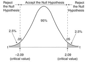
Figure 5.2 One- and two-tailed tests (source: Redrawn and adapted from Cohen and Holliday 1982).
If taken calmly and carefully, most students and researchers are able to perform the mechanics of the statistical tests considered below without difficulty. However, choosing the right test to use in a given analytical situation is more difficult. Consider the following hypothetical question and answer section taken from Chatfield (1995):
Q: What do you want to do with your data?
A: A t-test.
Q: No, I mean why have you carried out this study and collected these data?
A: Because I want to do a t-test (with a puzzled look).
Q: No. I mean what is your prior hypothesis? Why do you want to do a t-test?
A: My supervisor wants me to.
Q: No, I mean what is your objective in analysing these data?
A: To see if the results are significant. . .
The point here is that you do not undertake statistical tests in isolation, or test for significance in some arbitrary fashion. The main motivation for choosing a statistical test to apply to a set of data has to be driven by the objectives of your research project, and as indicated in Chapter 4, your project should have been designed and data sampled with a certain test or set of tests in mind. If not (for example, you may want to use secondary data that were collected by someone else or for another purpose), then you might like to consider the following questions modified from Chatfield (1995) to suggest an appropriate method (or methods):
The choice of an appropriate statistical test can be determined by a consideration of the number of samples, the type and nature of data you have collected. With reference to Section 5.1 above and then Table 5.2, we can categorise the tests discussed below in terms of being parametric/non-parametric (or dealing with a certain data type), in terms of the number of data samples, and whether we are interested in establishing differences or examining associations.
How do you decide whether to use a non-parametric or a parametric test? Clearly if you are using nominal or ordinal data you are restricted to non-parametric tests. If you wish to use a parametric test, you should try to establish whether your data conform to the assumptions required for such tests. Although we list the main assumptions for each test in Sections 5.6-5.7 below, the common characteristics of both parametric and non-parametric tests are listed in Box 5.2. The evaluation of your data should consider the normality of the distribution, the presence/impact of outliers, the homogeneity of variance and the sample size (Pett, 1997). Normality can be assessed in three ways. First you could calculate the skewness (degree of symmetry)
Box 5.2 Common characteristics of parametric and non-parametric tests
Source: Adapted from Pett 1997.
and kurtosis (flat or peaked shape) of the distribution. Next, you could plot the shape of a distribution, using the histogram, stem-and-leaf and box-and-whisker plots from Chapter 4. Finally, there are several statistical tests (e.g., the Shapiro-Wilks test of normality) which could be used to try to fit the data to a normal distribution. Outliers can be identified using box-and-whisker plots. The homogeneity of variance can be assessed by comparing the variances between subgroups. These should be similar: a formal statistical test (e.g., the Levene test) can be applied if necessary. Although it is generally agreed that small samples are inappropriate for parametric analysis, it is not clear from the literature what size is too small (Pett, 1997). For further details, you should consult one of the basic statistical texts listed at the end of this chapter. A clear treatment can be found in Pett (1997), in particular in Chapter 3, 'Evaluating the characteristics of data'.
However, if you are still not sure, useful advice is to try both the parametric and non-parametric tests where possible. If you get similar results you would be more likely to believe them; if not, you may have to look more closely at the assumptions concerning the data (Chatfield, 1995). Of course, if your data appear to violate some of the underlying assumptions, you might wish to use a data transformation (see Section 4.7), and then use the appropriate parametric test. Again, a possible course of action might be to apply the test before and after the transformation, and see if the result changes.
In Sections 5.6 and 5.7 we describe the mechanics of some of the more common and useful statistical tests. We have included the calculation of both parametric and non-parametric correlation coefficients, and linear regression, which all include the calculation of tests of significance for the coefficients. Note that the coverage of tests in this book is not exhaustive: in particular we have not included several nonparametric tests such as the Friedman, McNemar or Cochran's Q. For further details you should consult Pett (1997) or Coshall (1989) for examples in a geographical context.
Methods are divided into parametric and their nonparametric equivalents. For each technique we have adopted a common format, similar to that used in Chapter 4:

If you know what type of test you wish to perform, we advise that you read through fully all of the above sections for the appropriate test, particularly the step-by-step description of the test and the explanation. Step-by-step details are also given for doing the calculations by hand and using the MINITAB statistical package. Even if you intend only to use MINITAB, it is often useful to have some experience of performing the calculations by hand - if only for the worked example, to understand how the test works. To understand the distinction between certain tests, you might have to read this section or indeed the chapter fully, but by this time we hope that you should understand the major elements of significance testing so that you are able to select, execute and interpret the results of an appropriate test.
We would like to encourage the use of the IDA techniques outlined in Chapter 4 as an essential preliminary to each test described below. This is mainly for two reasons. First, each test makes assumptions about the data being analysed. Parametric tests in particular make certain assumptions about the data distribution. Although some tests are robust and resistant to outliers in the data and non-normal distributions,
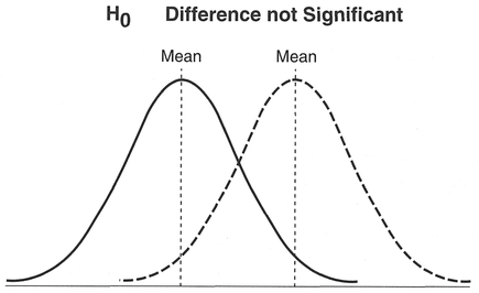
Figure 5.3 Differences in means and populations.
IDA techniques will help to establish whether or not the assumptions made about the data for each test appear to be warranted. This may well influence your choice of test, and we will discuss this further below. Second, the use of appropriate IDA techniques will give you a better understanding of, and feel for, your data, which can be helpful in determining whether you need a formal test at all, and perhaps more importantly will give you a good idea to anticipate what the results of any given test might be (Wright, 1997). Differences between groups may be so large as to be obvious without a test, and anticipating the results can help avoid errors in calculation.
Experimental design: Independent data sets.
Level of data: Interval/ratio.
Type of test: Parametric.
Function: Test of difference.
What the test does: Compares two unrelated data sets by inspecting the amount of difference between their means and taking into account the variability (spread) of each data set.
Assumptions:
Explanation and procedure: With two groups of data, a two-sample f-test is used to determine if the difference in means is significant. The t-test used here is a comparison between two sample means allowing for the variability in the data. This is in the form:

The larger the difference in the means, the more likely that a real, significant difference exists, and our samples come from different populations (Figure 5.3).
We do not have any information about the population variances (if we did, we could use a Z-test: see Section 4.6).
Lay out the data such that you can calculate the squares of each case, or enter data into the MINITAB spreadsheet (Step 1). It is vital that you summarise and check the data for the presence of outliers or errors before starting to use the methods described in Chapter 4. Extreme values in the data could dramatically affect the results of a t-test, and could indicate that the data come from a non-normal distribution. If such values do not appear to exist, we can proceed with the test. Proceed with checking the assumptions, and the calculation of sample variances using sums, means and squares (Steps 3-7).
An important preliminary step is to determine whether the sample variances for each group are equal, for which we use an F-test (Steps 8 and 9). The variances are calculated for each group, and then the value of F is obtained:

The next step is to compare the calculated value of F with a critical value of F at the 0.05 significance level with DF = n — 1 for each sample (Step 10). If the calculated F is greater than the critical value, the variances of each sample are significantly different. If the variances are significantly different, substitute the mean and variance and number of samples for each data set into the following formula to estimate t:

where x̄a, x̄b = mean,  = variance, and na, nb = number of samples of data sets A and B respectively. If the variances are not significantly different, a pooled variance can be used. Substitute the mean and variance and number of samples for each data set into the following formula to calculate t:

If the pooled variance has been used in Step 11 then calculate the degrees of freedom (DF) = na + nb - 2 (Step 12). Otherwise, the DF can be calculated as follows:
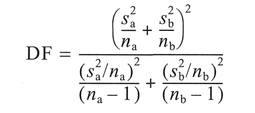
Lastly, check the critical value of t at the 0.05 significance level. If the calculated value of t is greater than the critical value, it is significant and we can reject the null hypothesis H0 (Step 13).
To illustrate the t-test, we will make use of the data set in Table 5.3 on domestic household waste production. The calculations are given in Boxes 5.3 and 5.4.
| Null hypothesis H0: μ1 = μ2 |
There is no difference between the quantity of domestic waste produced from households using bags and the quantity produced from households using bins. |
| Research hypothesis H1: μ1 > μ2 |
Households using bins produce a larger quantity of waste than households using bags. |
| Significance level: | 0.05. |
Interpretation: In the example above, the results of the F-test indicate that the sample variances are equal
Box 5.3 Handworked example: unrelated t-test

 (columns 2, 4, 6 and 8 in the table above).
 column by adding together all the data values, and call the sum Xx2. Repeat for
 Step 8 Calculate the variance of each data set (see Section 4.5.4):


Box 5.4 MINITAB example: unrelated t-test
Enter the bag data into C1 and the bin data into C2.

MINITAB results:
MINITAB will place the calculations for the variance of C1, C2 in C3 (= 80.30) and C4 (= 50.58), and the calculation of F in C5 = 1.587.

MINITAB results:
Inverse Cumulative Distribution Function
F distribution with 34 d.f. in numerator and 31 d.f. in denominator
| P(X <= x) | x |
|---|---|
| 0.9500 | 1.8055 |

MINITAB results:
| MTB > two-sample c1 c2; |
| SUBC > pooled. |
Two Sample T-Test and Confidence Interval
Twosample T for C1 vs C2
| N | Mean | StDev | SE Mean | |
|---|---|---|---|---|
| C1 | 35 | 12.13 | 8.96 | 1.5 |
| C2 | 32 | 16.95 | 7.11 | 1.3 |
95% C.I. for mu C1 - mu C2: ( -8.8, -0.8)
T-Test mu C1 = mu C2 (vs not =): T = -2.42 P = 0.018 DF = 65
Both use Pooled StDev = 8.13

at the 0.05 significance level, and the calculation of t using the 'pooled' estimate produces a calculated value of t which exceeds the one-tailed critical value at the 0.05 significance level. The MINITAB results produce p = 0.018, which confirms the handworked result. We reject the null hypothesis. It would appear that at the 0.05 significance level, households using bins produce a larger amount of waste than households using bags. However, we cannot say at this point as to why bins produce more waste. This would need further investigation.
Experimental design: Related data sets.
Level of data: Interval/ratio.
Type of test: Parametric.
Function: Test of difference.
What the test does: Compares the actual size of differences between the matched/related scores in each condition or time. The test uses the mean difference for the group and also individual variation in the size of the differences for individual related pairs to compare data sets.
Assumptions:
Explanation and procedure: In contrast to the test above, this is a one-sample t-test for use with related data, which are also termed 'matched pairs' data. Generally, the analysis of data in terms of matched pairs is more powerful because the design of a matched pairs scheme minimises unwanted 'background' variability which might be present in an independent randomised sampling scheme (Heath, 1995). This is reflected by a decrease in the standard error (denominator) of the t-test equation:

The mechanics of the test are very similar to those of the standard t-test described above, except that we are concerned with the differences between each matched pair of data values from two groups.
To calculate the value of t by hand, lay out your data in two columns such that you can estimate the difference between each matched pair of values (Step 1). MINITAB will also require you to enter your data into the spreadsheet in this fashion, as you will have to obtain the differences similarly to the handworked method. Summarise and check the data for normality and outliers, and consider the use of a non-parametric technique or transformation of the variables. Next, calculate the mean of each group (Step 2). Then obtain the differences by subtracting each paired value from the group with the smaller mean from the corresponding paired value of the group with the larger mean. Insert this column into the data set. Square each of these differences to create another new column in the data set (Step 3). Proceed with the calculation of the sum of the differences (Step 4), and then the calculation of the standard deviation of those differences (Steps 5 and 6). Next calculate the value of t using the following formula (Step 7):

where d = the differences, and n = number of observations. Then determine the degrees of freedom (Step 8). Finally, obtain the tabulated critical value of t at the 0.05 level for comparison - Table A.2 in Appendix A (Step 9). If the calculated value of t is greater than the critical value, it is significant and we can reject the null hypothesis H0- we can be 95% confident that there is a significant difference between the two data sets.
To illustrate the related t-test, we have used data (Table 5.4) on occupied office space in the US, from Sui and Wheeler (1993): see Boxes 5.5 and 5.6.
| Null hypothesis H0: μ1 = μ2 |
There is no significant difference between the growth rates of occupied office space in large metropolitan areas in 1985 and 1990. |
| Research hypothesis H1: μ1 ≠ μ2 |
There is a significant difference between the growth rates of occupied office space in large metropolitan areas in 1985 and 1990. |
| Significance level: | 0.05. |
Box 5.5 Handworked example: related t-test


Box 5.6 MINITAB example: related t-test
Enter the 1985 location quotient into C1 and the 1990 location quotient into C2. Calculate the difference between the two data sets by subtracting the data set with the lower mean from the other (e.g., Type: Let C3 = C1 - C2).

MINITAB results:
MTB > ttest 0 C3
Test of MU = 0.0000 vs MU N.E. 0.0000

Interpretation: In the example above, the calculated value of t is less than the critical value of t at the 0.05 significance level. The MINITAB results produce p = 0.094 which confirms the handworked result. We therefore fail to reject the null hypothesis. At the 0.05 significance level, there is no significant difference between the growth rates of occupied office space in large metropolitan areas in the US in 1985 and 1990 (note that there is a difference at the 0.1 level).
Experimental design: Independent data sets.
Level of data: Interval/ratio.
Type of test: Parametric.
Function: Test of difference.
What the test does: The test examines the differences between three or more groups by looking at each group mean. The null hypothesis H0 states that there is no difference between group means and any differences have been generated by chance.
Assumptions:
Explanation and procedure: If you have data which are classified into groups and you want to find out if the means of each are different, you perform an analysis of variance (ANOVA). Why not just do lots of i-tests? If you use 0.05 as the significance level, the probability of getting a significant result using a Mest when there is really no difference between the means is 5%. But if you make multiple comparisons, say between 10 pairs of means, then the probability of getting a significant result purely by chance is (Grant, personal communication):

If we pool all data - ignoring any classification into groups for the moment - we can calculate an overall total variance. This can be partitioned into two components: the variance between groups and the variance within groups (or residual variance). Here the model we are working from is:

The between-group variance is in the form of the squared deviations between each group mean and the global mean, known as the between-group sum of squares (SSB), which, divided by the degrees of freedom, gives the between-group mean square (MSB). Similarly, the within-group variance is obtained from the sum of squared deviations between each group observation and the group mean, known as the within-group sum of squares (SSW), which, divided by the degrees of freedom, gives the within-group mean square (MSW). The ratio between the MSB and the MSW is known as the F-test. This is approximately 1 when the null hypothesis H0 is true, since we are saying that we expect MSB = MSW = σ2. When there are large differences between group means, the MSB will be larger and the F-ratio will be larger than one. The differences in means and distributions under both a null hypothesis and a research hypothesis for three groups are shown in Figure 5.4.
The analysis of variance makes several assumptions about the data. The variance within each group is similar; the data are normally distributed and come from an independent random sample. You should organise your data into a table (Step 1) and perform an IDA on the groups to check these assumptions prior to launching into an ANOVA. Individual group standard deviations can be compared but it is often sufficient to compare the mean, median and range (Step 2). Note that with small groups the range may be used to measure spread rather than the standard deviation. It may be useful to examine the results graphically using a box-and-whisker plot for each group. This may also reveal group differences to be obvious, which may indicate that an ANOVA is not necessary (Step 3). Small variations between groups are not too important. Targer variations between groups can be dealt with by a data transformation as explained in Chapter 4 (Step 4), or by the adoption of a non-parametric technique such as the Kruskal-Wallis test rather than ANOVA.
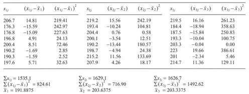
The within-group sum of squares (SSW) (Step 5) is defined as:

where x1j is each observation in group 1, and x̄1 is the mean for group 1. The SSWs of all groups are then added together. The between-group sum of squares (SSB) (Step 6) is defined as:

where x̄i is the mean of each group of ni values. We can divide the SSB and the SSW by the between-group degrees of freedom (k -1) and the within-group DF (n - k) (Step 7), where n denotes the total number of observations to obtain the mean square (MS) (Step 8) for the group means:

and within each group:

The F-statistic is calculated (Step 9) from:

The results of an ANOVA are usually presented in the following form (Step 10):
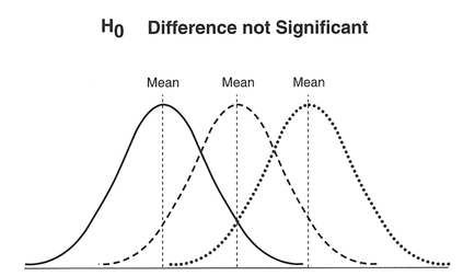
Figure 5.4 Differences in means and populations for the analysis of variance.
| Source of variation | DF | SS | MS | F |
|---|---|---|---|---|
| Between groups | k - 1 | SSB | SSB/(k - 1) | MSB/MSW |
| Within groups | n - k | SSW | SSW/(n - k) | |
| Total | n - 1 | SSB + SSW |
Note that the within- and between-groups of variation are additive and will sum to the total sum of squares, as will the degrees of freedom. This provides a useful check on the calculations. If F < 1, there is less variation among the means than you would have expected by chance, and you have obtained a nonsignificant result. For F > 1, using DF1 = (k - 1) and DF2 = (n - k), look up the critical value of F from a table of percentage points of F distribution at 0.05 level (see Table A.1, Appendix A) (Step 11) and determine whether or not the H0 can be rejected (Step 12).
If the ANOVA produces a significant result, how do we tell which groups are different from each other? There are a variety of tests which can be used, termed multiple comparison tests (see Sokal and Rohlf, 1995, for a survey), the choice of which depends initially on whether you are making planned comparisons (a priori) which are planned before we perform the sampling and ANOVA. In this case, if the number of comparisons is orthogonal it is simply a matter of performing a modified t-test for each comparison, but if the number of comparisons is nonorthogonal, the overall error rate must be proportionally reduced: see Sokal and Rohlf (1995) and Wright (1997) for details. If, however, you are not sure what comparisons to make in advance of performing the test, you need to adopt an unplanned comparisons (a posteriori) procedure. Again, there are a variety of methods which can be used here, one of the more popular being known as 'Tukey's honestly significant difference method' - the Tukey test for short - which is the simplest method to use, ideally in the presence of equal sample sizes. The idea is to obtain a critical difference based on sample characteristics and a critical look-up value. For this a parameter T can be defined as follows:

where Q is a special statistic for significance testing called the studentised range. The parameter Q is obtained at the 0.05 level using the number of groups k and DF = (n - k) (see Table A.3, Appendix A).
Substitute Q into the equation above to calculate T. If the difference between any pair of means (e.g., x̄1 — x̄2) exceeds or equals T then those means are significantly different.
As an example, Table 5.5 details the total distance estimates by blind individuals A—H between a number of locations along a route after walking the route on three separate (trial) occasions. The data were generated using a ratio-scaling technique, where respondents are given a ruler which represents the total length of the route and are asked to estimate the length between pairs of locations as a proportion of the ruler's length. Boxes 5.7 and 5.8 show the calculations.
| Null hypothesis H0: μ1 = μ2 |
There is no significant difference between the distance estimates of blind people on different trials. |
| Research hypothesis H1: μ1 ≠ μ2 |
There is a significant difference between the distance estimates of blind people on different trials. |
| Significance level: | 0.05. |
Interpretation: In our example above, the F value did not exceed the critical value at the 0.05 significance level, and the MINITAB results produce p = 0.108. This means that the sample variances of the data within each condition (trial) did not differ significantly. Note that, although the value of F is not significant, we have produced the results for the Tukey test to give an example of the MINITAB output. Since all of the pair comparison confidence intervals contain a zero, we deduce that none of the pairs is significantly different - not a surprise, given the test results. Given that the respondents were learning a new route, and that the trials represented the first three times this route was walked, we might expect there to be a significant difference between trials as respondents' knowledge of the relative distances between places increased. The fact that we have not found such a difference can be interpreted in two ways: (1) either it takes longer than three trials before there are significant increases in the accuracy of distance estimation, or (2) the respondents were very accurate in their responses, right from the first trial. The only way to determine this is through further testing, relating all (remember we have used only the totals) the cognitive estimates of the blind respondents to the real distances. Such analysis has been performed by Jacobson et al. (1998) using linear regression (see below), and revealed that, contrary to what might be thought, blind respondents were very accurate in their distance estimations, right from the first trial.
Experimental design: Independent data sets.
Level of data: Interval/ratio.
Type of test: Parametric.
Function: Test of association.
What the test does: Determines if two variables are interdependent, i.e., the degree to which they vary together.
Assumptions:
Explanation and procedure: Pearson's product moment correlation coefficient provides a measure of the linear association between two variables and varies between -1 (perfect negative correlation) and +1 (perfect positive correlation). After laying out the data and checking the assumptions (Step 1), an important second step is to produce a scatter plot of one variable against the other to assess whether the calculation of a correlation is appropriate (Step 2). In simple terms Pearson's correlation coefficient is a ratio of the variance shared between the two variables to the overall variance of the two variables (Cramer, 1997):
Box 5.7 Handworked example: ANOVA

| Source of variation | DF | SS | MS | F |
|---|---|---|---|---|
| Between groups | 2 | 718.01 | 359.01 | 2.48 |
| Residual | 21 | 3034.13 | 144.48 | |
| Total | 23 | 3752.14 |
Box 5.8 MINITAB example: ANOVA
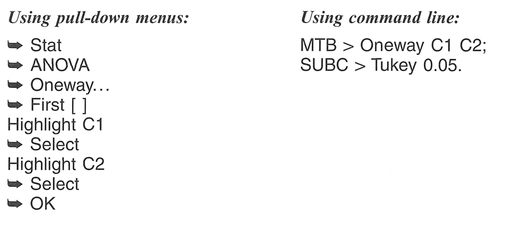
In MINITAB a one-way analysis of variance can be performed using the command 'aovoneway', which requires' each group to be in a separate column, or 'oneway' which has all data listed in the first column and the group membership in the second column. We will make use of the latter alternative. Note that MINITAB performs the Tukey multiple comparisons test by printing out a confidence interval for the population value of the difference between each pair of means. If this interval includes zero, the pair of means is not significant.
Place each length estimate into C1, placing a number representing the group membership (termed a subscript) in C2. For example:

MINITAB results:
One-way Analysis of Variance
| Analysis of Variance on 1 | |||||
|---|---|---|---|---|---|
| Source | DF | SS | MS | F | p |
| 2 | 2 | 718 | 359 | 2 .48 | 0 .108 |
| Error | 21 | 3034 | 144 | ||
| Total | 23 | 3752 | |||

Tukey's pairwise comparisons
| Family error rate | = | 0.0500 |
| Individual error rate | = | 0.0200 |
Critical value = 3.56
Intervals for (column level mean) - (row level mean)
| 1 | 2 | |
|---|---|---|
| 2 | -26.88 | |
| 3.38 | ||
| 3 | -2 6.58 | -14.83 |
| 3.68 | 15.43 |


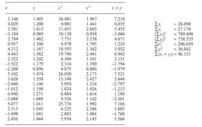
The covariance and variance are based on the difference between the scores and the mean of each variable, and the calculations to estimate covariance/ variance can be broken down into a number of simple steps. First (Step 3), create two new columns of data consisting of the square of each x score (i.e.,  in one) and the square of each y score (i.e.,
  in the other). Next (Step 4), create a fifth column of data by calculating the product of each x and y score (i.e., xi x yi). Calculate the sum Σxi of all the observed x scores and the sum Σyi of all the observed y scores (Step 5). Obtain the squares of these sums, i.e., (Σxi)2 and (Σyi)2 (Step 6), and sum the column of
  to give
  and similarly with
  to give
  (Step 7). Finally, sum the remaining column of xi X yi products to give Σ(xi x yi) (Step 8). The correlation coefficient r can then be calculated (Step 9):

If the variance shared between the two variables is high, then this ratio will approach either +1 or -1, i.e., a perfect positive or negative correlation. The significance of the ratio can be calculated by calculating t and looking up a value of t in Table A.2, Appendix A (Step 10), where:

The choice of a one- or two-tailed test will be dependent on the directionality (if any) of the research hypothesis.
As an example, we will use two variables selected from Table 5.6 (columns C2 and C6), compiled by researchers at the School of Environmental Sciences, University of East Anglia. We will make further use of the data in this table for demonstrating Spearman's correlation coefficient and linear regression later in this chapter. Boxes 5.9 and 5.10 show the calculations.
| Null hypothesis H0: μ1= μ2 |
There is no significant association between the child accident rate and the Townsend material deprivation score. |
| Research hypothesis H1: μ1≠ μ2 |
There is a positive association between the child accident rate and the Townsend material deprivation score. |
| Significance level: | 0.05. |
Interpretation: In the example, we have used data from Table 5.6 which is a data set collected to examine accidents to pre-school children (aged 0-4 years) and the influence of social variables in 21 areas in Norwich. The results above, correlating childhood accidents with the Townsend material deprivation score (see Townsend et al, 1988), produce an r = 0.807, and indicate a strong positive association between the two variables, which we might expect since childhood accidents are most common in households living in poor circumstances. Further, this positive association is significant at the 0.05 significance level.
Experimental design: Independent data sets.
Level of data: Interval/ratio.
Type of test: Parametric.
Function: Examining trends.
What the test does: Bivariate regression analysis is concerned with the prediction of the values of one variable, knowing the other, the estimation of causal relationships between two variables, and the description of functional relationships where only one of the variables is known exactly. Strictly speaking, it is not a test but rather seeks to examine trends within data. The expressions of the trend can, however, be tested for significance.
Assumptions:
Explanation and procedure: In the previous section, we examined how the strength of a bivariate relationship could be measured in terms of a correlation coefficient. However, we often need to know exactly how one variable varies with respect to another. This usually means that we have to fit a mathematical equation - often called a line of best fit - to the paired data values. Unless the two variables are perfectly correlated (i.e., fall on a straight line), there will be a degree of scatter between them and subsequently many different linear and non-linear mathematical equations can be fitted to the data. We will only consider linear equations within this chapter for situations where there are individual data points comprising each pair. You should make reference to a more specialised text such as Bates and Watts (1988) for details on fitting non-linear functions.
One group of techniques fits a linear function, described as a least-squares linear regression, on the basis of minimising the squared deviations between the data points and the function. Deviations can be minimised in either an x-direction, a v-direction or even perpendicular to the line of best fit. For a least-squares regression of the y variable on x, we would minimise the deviations in the y direction as seen in Figure 5.5.
The variables that we assign to x and y in this case depend on our understanding of the relationship between them. The variable we assign to x varies in either a known fashion (Type I regression) or an unknown independent fashion (Type II regression), but is somehow related to the variation observed in y. In other words, values of y are dependent on the values of x. Following convention, y refers to the dependent variable (also known as the response variable) and x refers to the independent variable (also known as the predictor variable). In the worked example above, we return to the data in Table 5.6 on child accidents in Norwich and focus on the Child
Box 5.9 Handworked example: Pearson's correlation coefficient
 and insert in column 3. Do the same for each y score to produce
  and insert in column 4.
 to give
  and similarly with
  to give


Box 5.10 MINITAB example: Pearson's correlation coefficient
From Table 5.6, place C2, 'Child Accident Rate', in C1; and C6, 'Townsend Material Deprivation Score', in C2. Transform CI by taking natural logs: place the result in C3. The 'plot' command (see Box 5.12) can be used to produce a scatterplot of one variable plotted against the other.

MINITAB results:
MTB > Correlation C2 C3.
Correlations (Pearson)
Correlation of C2 and C3 = 0.807

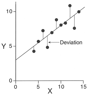
Figure 5.5 Least-squares regression.
Accident and Percentage Unemployed variables. In this case, the 'Percentage Unemployed' is the independent x variable, and 'Child Accidents' is the dependent y variable, which we think may somehow be linked to variations in the unemployment rate (which we are using as a surrogate for deprivation). In fact, the same could be said of any of the other variables in Table 5.6 other than Child Accidents: these variables were all selected as potential causal factors explaining the Child Accident variable. Establishing causal relationships constitutes one important use of linear regression in human geography.
The least-squares form of regression used here is appropriate only under specific circumstances: usually that the independent variable x is free of error, or if error exists it is known to be negligible. This is the Type I regression mentioned above, which we have described in this section. Where there are errors in both variables, a Type II regression is more appropriate. In this situation, other techniques for fitting functions to paired data, commonly known as structural analysis, are more appropriate, but are not discussed here.
We can model the data shown by the points in Figure 5.5 in terms of the relationship

where e = y - ŷ represents the deviations which we minimise. In contrast, the form of the equation fitted in Figure 5.5 is

We have discussed the meaning of the terms x and y, but the final two terms in the above equation also need to be explained. Both are constants and together they are known as regression coefficients. The a coefficient is the intercept, which is the value of y obtained when x is zero (i.e., when the line of best fit intercepts the y-axis). The b coefficient is the slope (gradient) of the line, which tells us how much change we will observe in the y variable with a specific change in the x variable.
To perform a linear regression we need to estimate the a and b coefficients in the equation above. For the b coefficient:

Note that the equations for the variance and covariance are equivalent to the definitions in Sections 4.5.4 and 5.6.4. We make use of an abbreviated form here. In order to be a best-fit line, the regression line must pass through the means of both the x and y variables, and once we have obtained b, the a coefficient can be obtained from

The model of variance in our regression is often expressed in a form similar to that used with the analysis of variance discussed earlier in this chapter:
| Sum of squares explained by the regression (RSS) | = | Total sum of squares (TSS) | + | Sum or squares unexplained by the regression (ESS) |
We can assess the goodness-of-fit of the linear regression by looking at the ratio of the total sum of squared deviations (TSS) to the sum of squared deviations explained by the regression (RSS), with the resulting parameter R2 known as the coefficient of determination. When the regression is a good description of the relationship, the two terms above will be similar in size and the value of R2 will be high. However, when the regression is a poor description of the relationship, the RSS will be small, as will the value of R2.
Once we have fitted a regression model, it is important to assess the significance of the estimated coefficients. It is possible to calculate the standard error around regression coefficients with associated confidence limits, and to perform tests of significance upon regression parameters. There are a variety of methods which can be used, and hypotheses which can be tested. For example, to test whether the regression coefficient b comes from a population where the population slope β = 0, we can also make use of a Student's t-test. To obtain the calculated value of t we make use of a form of the formula which we encountered with the Pearson correlation coefficient:

which can then be compared with the critical value of t at n — 2 degrees of freedom. If the calculated value of t exceeds this, then β is significantly different from 0. In a similar fashion the coefficient a can be tested to see if the population intercept α is significantly different from 0.
The calculation of standard errors and confidence limits should never be the final step in a regression analysis. The examination of the residuals in a least-squares linear regression can supply much useful information concerning the appropriateness of the linear model and insights into the structure of the data. Residuals are defined as

They are often converted into leveraged coefficients, and then calculated in a standardised form. One of the main aims of the analysis of residuals is to identify influential observations. Chatfield (1995) defines an influential observation as one whose removal would lead to substantial changes in the fitted regression model. Cook's distance D is a measure of the influence of individual observations: values of D which exceed 1 indicate that the observation is influential. In addition, residuals can be plotted against both the calculated fits, and the x and y variables. If the linear regression provides a good description of the data, such a plot should reveal no particular pattern, but it could reveal (1) a few much larger residuals which could be outliers; (2) a curved regression on fitted values; (3) change in the variability of residuals; and (4) a skewed or non-normal distribution of residuals.
The data displayed in Figure 5.6 have been taken from Anscombe (1973). Although they display four very different patterns, they produce the same R2 and the same regression parameters. The results presented here, although extreme, provide examples of the different effects which may make the final calculated regression parameters misleading. This demonstrates the necessity of not only carefully plotting both the x and y variables in the form of a scatterplot prior to the regression analysis, but also plotting the residuals after the analysis.
To calculate linear regression, first check the assumptions, and construct a scatterplot to determine if a linear model is appropriate (Step 1). Regression is often used inappropriately (see above for explanation). For each variable, sum and divide by the sample size n to obtain the means x̄ and ȳ . Obtain x2, y2 and x x y, and the respective sums of each: (Σx2),
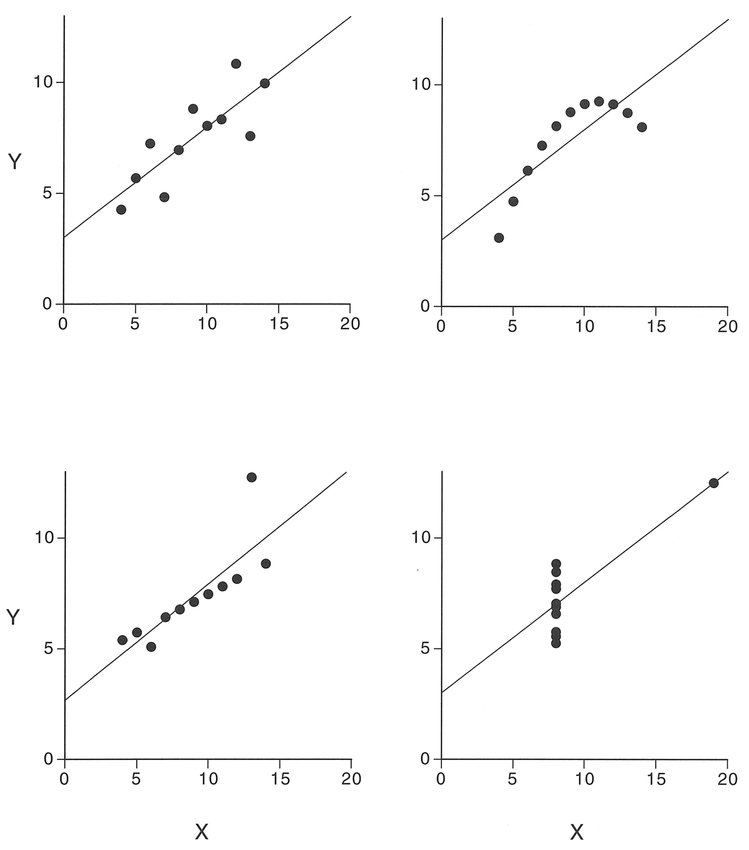
Figure 5.6 Patterns of residuals from a linear regression (redrawn from Anscombe 1973).
(Σy2) and (Σxy) (Step 2). Remember that x is the independent variable and y the dependent variable. To obtain the regression slope coefficient b, substitute into the following equation (Step 3):

Next calculate the intercept coefficient a by substituting into the following equation (Step 4):

The sum of squares explained by the regression (RSS) is obtained (Step 5) from:

and the sum of squares unexplained by the regression (ESS) is obtained (Step 6) from:

The total sum of squares (TSS) is most simply obtained (Step 7) from:

Finally, the coefficient of determination (R2) is obtained from:

Note: The following steps concern the estimation of the standard error and confidence limits around some of the regression coefficients calculated above and should be used only as required. Many of the quantities used have already been calculated, arid can simply be substituted into the appropriate equation.
The standard error (SE) around the slope coefficient b is calculated from the equation below (Step 8):

The 95% confidence limits around the slope can be obtained using the Student's t-distribution with the appropriate value of t obtained using n — 2 degrees of freedom:

We can then test the regression slope coefficient b, making use of the Student's t-distribution (Step 9) where the value of t is calculated from:

The standard error (SE) around the intercept a is calculated from the equation below (Step 10):

Again, the 95% confidence limits can be obtained using the Student's t-distribution with the appropriate value of t obtained using n — 2 degrees of freedom:

In a similar fashion to the b coefficient above, we then can test the intercept regression coefficient a:

Similarly we can calculate the standard error (SE) around the mean value of the dependent variable (Step 11):

with the 95% confidence limits obtained, again making use of the Student's t-distribution (as above):

As an example (Boxes 5.11 and 5.12), we will make use of data from Table 5.6, except this time we will examine the relationship between the child accident rate and the proportion of economically active males who are unemployed. Note that we will include the calculation and plotting of residuals from this regression only in the MINITAB example (Box 5.12).
Interpretation: The equation for the linear model is y = 0.974 + 2.90x, with an R2 of 57.6%. Note that the results of the significance tests for both the intercept and slope coefficients are significant at the 0.05 significance level. The advantage of linear regression over a measure of correlation is that we can predict a measure of y (in this case, the child accident rate) from a measure of x (in this case, unemployed economically active males). Note, however, that although the pattern of residuals shows no clear trend, the percentage of variation which is explained by the linear regression is only 57.6%, which still leaves some 42.4% unexplained. Although there is a significant linear relationship, we would not have considerable confidence in any predictions of y based on x. In fact, a more useful model would be constructed if we regressed the child accident rate against several of the variables from Table 5.6 in a multiple regression, although we will not consider this in this book. You should consult one of the more advanced texts listed at the end of this chapter for further details.
Box 5.11 Handworked example: linear regression


Then, to obtain the coefficient of determination (R2), substitute into the equation to give:


From Table A.2 in Appendix A, the two-tailed Student's t-value at a 0.05 significance level, using n - 2 = 19 degrees of freedom = 2.093; therefore the 95% confidence interval is:

i.e., from 1.70 to 4.09.

In this case, we compare this value with the two-tailed critical value at a 0.05 significance level with n - 2 degrees of freedom from above (2.093). The calculated value exceeds the critical value, therefore b is significantly different from zero.

For the 95% confidence interval substitute in SE(a) and the value of t from above (2.093)

i.e., from 0.83 to 1.12.

Again, we compare this value with the two-tailed critical value of t at n - 2 degrees of freedom from above (2.093). The calculated value considerably exceeds the critical value, therefore a is significantly different from zero.

with the 95% confidence interval:

i.e., from 1.22 to 1.37.
Box 5.12 MINITAB example: linear regression
In addition to the regression equation and R2, MINITAB provides as standard the SE ('StDev') and t tests for significance ('t-ratio') of the regression coefficients, as well as ANOVA statistics which could also be used for testing the coefficients. Any 'unusual' observations are also identified. In addition, we have requested residuals and fits to be stored in columns C4 and C5. We will only graph fits against residuals, although you should also consider graphing residuals against the original variables or producing a histogram of the residuals for further analysis.
Place the data for the proportion of economically active males unemployed in CI and the accident rate per 1000 days at risk in C2. Transform C2 using natural log, placing the results in C3.


MINITAB results:
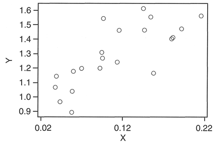
Figure 5.7 MINTAB output: scatterplot.

Analysis of Variance
| SOURCE | DF | SS | MS | F | p |
|---|---|---|---|---|---|
| Regression | 1 | 0.50286 | 0.50286 | 25.83 | 0.000 |
| Error | 19 | 0.36985 | 0.01947 | ||
| Total | 20 | 0.87270 |
Unusual Observations

R denotes an obs. with a large st. resid.
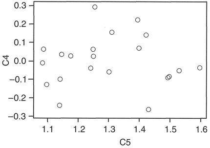
Figure 5.8 MINTAB output: residuals.
Experimental design: Frequency or count data.
Level of data: Nominal/categorical.
Type of test: Non-parametric.
Function: Comparing proportions.
What the test does: This test helps to establish whether there is a significant difference in the distribution of data between two or more variables or whether any differences are due to chance. A comparison is made of observed frequencies with the expected frequencies if chance is the only factor operating.
Assumptions:
Explanation and procedure: The first step (Step 1) is to check whether the data satisfy the test assumptions. Then assemble the data into a contingency table consisting of the categories of one variable for each row i against the categories of the other variable for each column j, with the observed frequency O in each cell. Next (Step 2), sum the total of observed frequencies Oij for each row i and column j. Obtain the grand total, checking that this is the same for summing all rows as for summing all columns. Once Steps 1 and 3 are completed, you may suspect that your data follow a trend: there may appear to be more counts in one category than another. But how large do the differences have to be in order to be significant and not to have arisen by chance? The chi-square goodness-of-fit test allows you to test whether any observed differences in your data table are in fact significant. More specifically, it tests the null hypothesis H0 that 'rows and columns are independent', in other words that the probability of an observation Oij falling in any particular column j does not depend on the row i the observation is in (and vice versa) (Chatfield, 1995).
The test is based on estimating the expected frequency Eij of observations in each cell. This is obtained by distributing the data according to the proportions each row and column make with the overall total (Step 3). Eijis calculated for each cell by multiplying the row total by the column total and dividing by the grand total, i.e.:
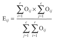
Now, examine the distribution of expected frequencies Ey. If more than 20% of the expected values are less than 5, merge these categories with adjacent, related categories in the table and then recalculate the expected frequencies (Step 4). This formula calculates the difference between the observed and expected frequencies, squaring the result and then dividing by the expected frequency. Calculate the total degrees of freedom (DF) available, which for a 1 x 1 table is (number of columns - 1) or for a 2 x 2 (or greater) table is (number of rows - 1) x (number of columns - 1) (Step 5). If DF > 1, calculate the chi-square statistic using the standard formula as follows. For each cell take the absolute difference between the observed and expected cell values Oij Eij (Step 6). Take the square of the result and sum together for all cell values:

A further correction is made if you are using a small 2x2 table: this is termed Yates' continuity correction (Step 7). This is necessary because the chi-square statistic is derived from the continuous probability distribution, which is being used as an approximation to the discrete probability distribution of observed frequencies. The calculation of χ2 is the same as in Step 6 except for the subtraction of 0.5 from Oij - Eij:

If the sample size is reasonably large this correction has little effect, and the standard formula should be used (see Step 6). Once applied to each cell in the table, the results are then summed to produce a calculated value of chi-square (χ2) which can then be compared against the critical value of χ2 (see Table A.4, Appendix A) (Step 8). The chi-square test is a one-tailed test since differences will always lead to a large value of χ2 (Chatfield, 1995). If the calculated value of the chi-square statistic is greater than the critical value, the null hypothesis H0 can be rejected and it can be concluded that there is a significant association between the variables (Step 9). Everitt (1992) provides an exhaustive summary of the analysis of contingency tables, including alternatives to pooling
Table 5.7 Household head income (weekly) by dwelling type for those aged under 65 m Aberdeen.
| Multi-storey and flatted | Tenement | Terraced and semi-detached | Total | |
|---|---|---|---|---|
| Under £50 | 18 | 20 | 12 | 50 |
| £50-£74 | 13 | 18 | 20 | 51 |
| £75-£99 | 23 | 19 | 45 | 87 |
| £100+ | 21 | 30 | 58 | 109 |
Source: Williams et al., 1986.

Box 5.13 Handworked example: chi-square
| Multi-storey and flatted | Tenement | Terraced and semi-detached | Total | |
|---|---|---|---|---|
| Under £50 | 18 | 20 | 12 | 50 |
| £50-£74 | 13 | 18 | 20 | 51 |
| £75-£99 | 23 | 19 | 45 | 87 |
| £100+ | 21 | 30 | 58 | 109 |


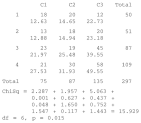
Box 5.14 MINITAB example: chi-square
Enter the income data into CI (Multi-storey), C2 (Tenement) and C3 (Terraced).

MINITAB results:
MTB > chisquare c1-c3.
Chi-Square Test
Expected counts are printed below observed counts

categories where the expected values are less than 5. Also, for a small 2x2 table, a simplified version of the χ2 formula may be used (see Everitt, 1992, Section 2.3).
To illustrate this test, we will use a data set (Table 5.7) which compares dwelling type against income for a sample of those aged under 65 in Aberdeen: see Boxes 5.13 and 5.14.
| Null hypothesis H0: |
Dwelling type is independent of tenant income (i.e., there is no significant difference in tenant income with dwelling type). |
| Research hypothesis H1: |
Dwelling type depends on tenant income (i.e., there is a significant difference in tenant income with a change in dwelling type). |
| Significance level: | 0.05. |

Interpretation: In the handworked example above, the calculated value of chi-square exceeds the critical value and is therefore significant at the 0.05 significance level. Similarly, using MINITAB we obtain p = 0.015, which is less than 0.05 and therefore significant. We
can reject the null hypothesis H0 and be 95% certain that dwelling type depends on tenant income.
Experimental design: Frequency data in ordered classes (one or two samples).
Level of data: Ordinal.
Type of test: Non-parametric.
Function: Comparing distributions.
What the test does: Compares the data sample with some expected population distribution (one sample) or compares the distributions of two data samples.
Assumptions:
Explanation and procedure: The Kolmogorov-Smirnov test can be used with both a single sample and two samples. In the single-sample case, it is used to determine whether the goodness of fit of a sample is similar to a particular distribution, i.e., whether the observed frequencies of the sample coincide with what we would expect given a particular probability distribution. In the two-sample case, we are assessing whether the populations from which the samples have been drawn differ. Coshall (1989: 17) notes that the Kolmogorov-Smirnov test makes more complete use of the available data than the chi-square test, as it does not require the 'lumping together' of categories, and because it takes advantage of the ordinal nature of the data. That said, it is rarely used in human geography applications.
The Kolmogorov-Smirnov test makes use of the cumulative frequency (or probability) distribution. The first step in the analysis is to assemble the data for each sample in a frequency form, which should be placed in an ordered table (Step 1) and then in cumulative frequency form (Step 2). The cumulative frequency proportions are obtained by dividing the cumulative frequencies by the total number of observations in each sample (Step 3). The absolute differences between the cumulative frequency proportions for each column are obtained (Step 4) with the D statistic defined as the maximum value of the differences (Step 5). The critical value of D (at the 0.05 significance level) is obtained from a table of critical values (Table A.5, Appendix A) or, if either sample size n is greater than 25, from the equation (Step 6):

If the calculated value of D exceeds the critical value, then the null hypothesis is rejected (Step 7).
As an example data set, we have made use of the waste data from Table 5.3 above expressed in terms of class frequencies (see Table 5.8): see Boxes 5.15 and 5.16.
| Null hypothesis H0: |
There is no significant difference between the quantity of domestic waste produced from households using bags and that from households using bins: the samples come from similar distributions. |
| Research hypothesis H1: |
There is a significant difference between the quantity of domestic waste produced from households using bags and that from households using bins: the samples come from different distributions. |
| Significance level: | 0.05. |
Interpretation: From the data listed above, we find that at the 0.05 significance level, the two distributions do differ significantly, which matches the result obtained for the unrelated West above (Section 5.6.1). Pett (1997) notes that this test has the advantage over the t-test in that it compares the entire distribution, not just measures of central tendency.
Experimental design: Independent data sets.
Level of data: At least ordinal.
Type of test: Non-parametric.
Function: Comparison.
Box 5.15 Handworked example: Kolmogorov—Smirnov


Box 5.16 MINITAB example: Kolmogorov—Smirnov
MINITAB does not perform a Kolmogorov-Smirnov test as of version 10.1. However, you can get the software to do most of the hard work for you, and if either sample size exceeds 25, you can also calculate the critical value of D. Place Set A in CI and Set B in C2.

Repeat for C4, C5 and C6, substituting the expressions listed for the command line instructions above.
MINITAB results:
The calculated D statistic will be in C5 (0.35) and the critical value of D will be in C6 (0.3326).

What the test does: Determines whether two independent samples are from the same population. The scores in each data set are compared by ranking the individual scores and determining whether the ranks are evenly divided.
Assumptions:
Explanation and procedure: The Mann-Whitney U test is the non-parametric counterpart of the t-test for unrelated (independent) data. The test is used to determine whether ordinal data collected in two different samples differ significantly. For example, we might want to determine whether towns in two different regions have differing mortality rates or whether men and women assign the same familiarity ratings to an area. The test calculates whether there is a significant difference in the distribution (based on the median) of data by comparing the ranks of each data set.
The first step in the calculation is to check whether the data fulfils the test assumptions (Step 1). Next, rank all data as if one group giving the lowest score are ranked as 1. At this stage maintain group identity (Step 2). Now, find the sums Ra and Rb of the ranks in data sets A and B. For example, for set A (Step 3):

where na is the number of values in data set A. If these sums differ substantially, then there is reason to suspect that the two samples come from different populations (Pett, 1997). Then calculate Us for the smaller sample using the following formula (Step 4):

where R1 is the sum of ranks for the smaller sample, n1 is the size of the smaller sample, and n2 is the size of the larger.
Calculate U1 for the larger sample:

Select the smaller of Us and U1 and call it U (Step 5). Check the critical value of U in Table A.8, Appendix A (Step 6). If U is less than the critical value it is significant and we can reject the null hypothesis there is a significant difference between the two data sets. If one or both samples are greater than 20, convert the U value into a Z-score using the formula:

When ties occur between the ranked observations of two samples, the Z-score can be adjusted as follows:

where  tj is the number of observations tied at a particular rank j, and N is the total number of observations in both samples. The significance of Z is assessed by checking the Z-score in the critical table (Table A.8, Appendix A). The test is illustrated by a data set (Table 5.9) comparing the performance of football teams in the UK before and after a merger in 1921: see Boxes 5.17 and 5.18.
| Null hypothesis H0: |
Teams from the old Southern and Northern Leagues have not differed significantly in their success since 1921. |
| Research hypothesis H1: |
There is a significant difference in the degree of success enjoyed by teams from the old Southern and Northern Leagues since 1921. |
| Significance level: | 0.05. |
Interpretation: These results (see Boxes 5.17 and 5.18) reveal that the two data sets are significantly different, and we can reject the null hypothesis at the 0.05 significance level. The MINITAB results reveal that if these data are two independent random samples, the median of data set A (Southern) is between -41.0 and -16.99 units higher/lower than the median of data set B (Northern) and that the chance of observing two samples as separated as these, when in fact the populations from which they are drawn do not differ, is only 0.0004. We can therefore be confident that the teams from the old Southern and Northern Leagues have differed in their success since 1921. Note that we cannot say why, only that we are 95% confident that there is a difference.
Box 5.17 Handworked example: Mann—Whitney U test


Box 5.18 MINITAB example: Mann—Whitney U test
Enter the test data into the Data Screen with the Southern League data entered into CI and the Division 3 (North) entered into C2. Return to the MINITAB environment and using either the pull-down menus or command line calculate the Mann-Whitney statistic.
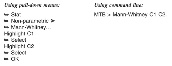
MINITAB results:
MTB > mann-whitney c1 c2.
Mann-Whitney Confidence Interval and Test
| C1 | N = 20 | Median = 18.50 |
| C2 | N = 18 | Median = 47.50 |
Point estimate for ETA1-ETA2 is -29.00
95.2 Percent C.I. for ETA1-ETA2 is (-41.00, -15.00)
W = 269.0
Test of ETA1 = ETA2 vs. ETA1 > ETA2 is significant at 0.0004
The test is significant at 0.0004 (adjusted for ties)
Experimental design: Related data sets.
Level of data: At least ordinal.
Type of test: Non-parametric.
Function: Comparison.
What the test does: The test examines the differences between data from the same phenomenon collected in two different conditions or times by examining the ranks of the difference in values over the two conditions.
Assumptions:
Explanation and procedure: The Wilcoxon signed ranks test is the non-parametric counterpart of the t-test for related data or paired t-test. The test is used to determine whether ordinal data collected from the same phenomenon differ between conditions or times. For example, we may want to know whether a town's mortality rate changes significantly between dates or whether the conditions under which a questionnaire or interview is conducted influence the findings of a study significantly. The test calculates whether there is a significant difference by examining whether the ranks of individual phenomena differ between conditions or times.
To calculate a Wilcoxon signed ranks test, first check the test assumptions (Step 1). If the test assumptions are met then calculate the difference between the two sets of data by subtracting one data set from the other (Step 2). Next, calculate the rank of the differences, ignoring the sign (-/+) of the difference. Any pairs with zero values should be ignored and omitted from the ranking and further analysis. When two or more differences have the same rank, take the average of the ranks they would have received had they differed and assign this average to each (Step 3). Sum the ranks for each sign, with the smaller of the two assigned to T (Step 4). Check the critical value of T in Table A.6, Appendix A (Step 5). Remember that n is the number of samples in the data set minus the number of entries where there was no difference between the two data sets. If T is less than the critical value it is significant at that level and we can reject the null hypothesis H0, i.e., there is a significant difference between the two data sets. If the number of samples n exceeds the table limits, the T value has to be transformed to a Z-score using the formula (Cohen and Holliday, 1982):

When extensive ties occur between ranks (e.g., the majority of the data are assigned to the same five or six tied ranks) then a correlation factor is introduced:
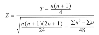
where u is the total number of tied ranks. The significance of Z is assessed by checking the Z-score in critical Table A.7, Appendix A.
To illustrate this test, we will examine the scores obtained by individuals participating in a sketch map exercise (Table 5.10): see Boxes 5.19 and 5.20.
| Null hypothesis H0: |
There is no significant difference between median sketch map scores in each of the two conditions. |
| Research hypothesis H1: |
There is a significant difference between median sketch map scores in each of the two conditions. |
| Significance level: | 0.05. |
Interpretation: From our calculations we can conclude that at the 0.05 significance level there is a difference between the performance of respondents in interview and non-interview conditions, and that this difference did not occur by chance. This is confirmed by the MINITAB test, with p = 0.041. Note that this result tells us only that there is a significant difference but tells us nothing about why the difference has occurred.
Experimental design: Three or more samples.
Level of data: At least ordinal.
Type of test: Non-parametric.
Function: Comparison.
Assumptions:
Explanation and procedure: The Kruskal-Walhs test is the non-parametric equivalent to the one-way ANOVA test discussed in Section 5.6.3. This test requires that we rank all data from the largest to the smallest ignoring group subdivision, and average those ranks which are tied. Similar to the Mann-Whitney U test discussed above, if the populations from which we have sampled are not significantly different, we would expect that the rank sums for each group would be approximately the same.
The first step in the calculation is to check the assumptions and lay out the data in a table (Step 1). Next, rank all the observations taken together as one group where the lowest rank = 1 (Step 2). For tied ranks, allocate the average rank to each tie. Now create new columns in the data table and enter the ranks (Step 3). Sum the ranks separately for each group k to give Rk, using the formula (Step 4):

where nk is the number of observations in group k. Next, substitute into the following formula to calculate H (Step 5):

Box 5.19 Handworked example: Wilcoxon signed ranks test
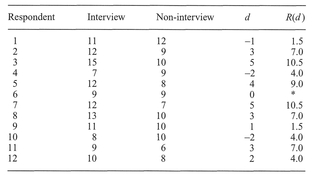

Box 5.20 MINITAB example: Wilcoxon signed ranks test
Enter the interview data into C1 and the non-interview data into C2. Then calculate the differences between the two and store in C3: C3 = C1 - C2. We want the two-tailed statistic, so we select 'not equal to' in the menu sequence below. You would select 'less than' or 'greater than' if you were performing a one-tailed test. The equivalent selection at the command line is 'Alternative 0' for a two-tailed test, with the replacement of the '0' with a -1 or +1 for a one-tailed test. Note that MINITAB reports the larger sum of ranks as the Wilcoxon statistic. Some statistics packages and tables are based on this sum rather than the smaller sum.
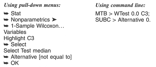
MINITAB results:
Wilcoxon Signed Ranks Test
| TEST OF MEDIAN = 0.000000 | VERSUS MEDIAN N.E. 0.000000 | ||||
|---|---|---|---|---|---|
| N | N FOR TEST | WILCOXON STATISTIC | P-VALUE | ESTIMATED MEDIAN | |
| C3 | 12 | 11 | 56.5 | 0.041 | 1.750 |
where n = total number of all ranks. If there are tied scores, the formula in Step 5 must be adjusted. Otherwise, go straight to Step 9. For each tie, the number of observations included in the tie t is used to obtain the parameter T. For each group of ties j, the parameter  is calculated from (tj - 1) x tj x (tj + 1) (Step 6). Sum together all the Tj, and substitute into the following equation to calculate parameter D (Step 7):

where m = the number of groups of ties.
Now calculate the corrected value of H by dividing by D (Step 8). Compare this with a critical value of χ2 (see Table A.4, Appendix A) and if H exceeds this critical value then reject the null hypothesis - there is a significant difference between the two data sets (Step 9). Similar to an analysis of variance, this does not tell you which groups are significantly different. To do this requires a similar post hoc approach to multiple comparisons as used in ANOVA, with a variety of options available. The Mann-Whitney U test can be used to establish whether pairs of groups are significantly different (Pett, 1997: 219). The reader is directed to Coshall (1988) or Pett (1997) for further details.
The data set we have chosen to illustrate the Kruskal-Wallis test is a set of data (Table 5.11) collected by Coshall (1988) to examine the trends between numbers of retail outlets and population: see Boxes 5.21 and 5.22.
| Null hypothesis H0: |
There are no significant differences in the numbers of retail outlets in the four samples of towns of varying population sizes. |
| Research hypothesis H1: | There is a significant difference in the numbers of retail outlets in the samples of varying population sizes. |
| Significance level: | 0.05. |
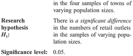
Interpretation: In our handworked example, the null hypothesis is rejected, and we can conclude that at the 0.05 significance level there is a significant difference in the numbers of retail outlets in the towns when classified according to their population sizes. Note how marginal the results are: MINITAB provides p = 0.049. Similar to the analysis of variance we cannot tell which pairs are different, only that a difference exists.
Experimental design: Independent data sets.
Level of data: Ordinal.
Type of test: Non-parametric.
Function: Comparison.
What the technique does: Describes the degree of association between two sets of ranked data.
Assumptions:
Explanation and procedure: Spearman's rank correlation coefficient (also known as Spearman's rho)
Box 5.21 Handworked example: Kruskal—Wallis
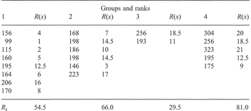


provides a measure of the linear association between two ranked variables and varies between -1 (perfect negative correlation) and +1 (perfect positive correlation). It is the non-parametric equivalent of Pearson's correlation coefficient discussed in Section 5.6.4. The basis of the statistic is the amount of disagreement between two sets of rankings. In simple terms, the value of the coefficient is a ratio of the actual amount of disagreement with the maximum possible amount of disagreement (e.g., when one rank order is the reverse of the other) subtracted from 1:

and is scaled so that r ranges from +1 to -1. The actual amount of disagreement is expressed in terms of differences between ranks, and the maximum possible disagreement is expressed directly in terms of sample size.
Box 5.22 MINITAB example: Kruskal—Wallis
Place the data in C1. Since the results are significant, the Mann-Whitney U test discussed earlier in this chapter can be used to establish which groups are different.

MINITAB results:


The first step (Step 1) in calculating Spearman's rank correlation coefficient is to plot the data in the form of a scatterplot of one variable against the other to assess whether the calculation of a correlation is appropriate. Next, create two new columns of data by ranking each of the variables separately, if not already in ranked form, giving a rank of 1 to the highest score (Step 2). Obtain the difference d between each pair of ranks and the difference squared d2, then sum the results to obtain Σd2 (Step 3). Now, calculate the denominator (n + 1) x n x (n - 1), where n is the number of values ranked (Step 4). If there are no tied ranks for each variable, calculate the correlation coefficient r using the following formula (Step 5):

However, if there are tied ranks on one or both of the variables then the formula becomes (Pett, 1997):

where the number of ties on each variable is obtained (e.g., for Tx) from:

with g = the number of groupings of tied ranks, and t = the number of ties in each group.
The calculated value of r will be -1 ≤ r ≤ 1 (Step 6). To test the significance of this result that the two variables are uncorrelated, we make use of the Student's t-distribution (Step 7):

Simply look up the value in Table A.2, Appendix A, at the appropriate significance level, using a one- or two-tailed test depending on the research hypothesis.
In the example detailed here, we make use of data from Table 5.6, concerned with child accidents and socio-economic characteristics for selected enumeration districts in Norwich. The example correlates child accident rate (x) with the proportion of households in rented accommodation (y): see Boxes 5.23 and 5.24.
| Null hypothesis H0: μ1 = μ2 |
There is no significant association between the child accident rate and the proportion of houses in rented accommodation. |
| Research hypothesis H1: μ1 ≠ μ2 |
There is a positive association between the child accident rate and the proportion of houses in rented accommodation. |
| Significance level: | 0.05. |
Interpretation: The calculated correlation coefficient between these variables is 0.777. A t-test is used to determine the significance, and in the example above, at the 0.05 significance level, we can reject the null hypothesis that the two variables are uncorrected: there is a significant positive association between the child accident rate and the proportion of houses in rented accommodation.
Many statisticians and researchers who use statistical methods are often uncomfortable about the widespread use of inferential statistical tests. This is often because of the specification of inappropriate hypotheses, the enforcement of rigid probability value p cutoffs, and the misinterpretation of the results of the statistical test. Chatfield (1995) notes that:
With respect to (1) we can produce significant effects in several ways: by selecting a research hypothesis which is obviously true, or a null hypothesis which is silly. Returning to the enumeration district example at the start of Section 5.3, would we really expect average income to be the same for two areas? Perhaps, but if the example used was for the city of Washington DC, and we selected enumeration district A on the east side of the city in an area with a predominantly low-income population, and enumeration district B in the west of the city in an area with a predominantly high-income population, we might

Box 5.23 Handworked example: Spearman's rank order correlation coefficient

Step 1 Produce a scatterplot of one variable against the other as shown in Figure 5.9.
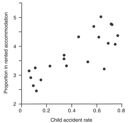
Figure 5.9 Scatterplot of child accidents against proportion in rented accommodation.


Box 5.24 MINITAB example: Spearman's rank order correlation coefficient
Place the child accident rate data in C1 and the proportion renting in C2. You should use the 'plot' command (explained in Box 5.12) to determine whether the two variables appear to be related. To perform a Spearman's rank correlation in MINITAB, you will first have to rank the data using the command 'rank', and then perform a product-moment correlation on the ranks.

MINITAB results:
| MTB > Rank C1 C3 . |
| MTB > Rank C2 C4. |
| MTB > Correlation C3 C4. |
| Correlation of C3 and C4 = 0.777 |
expect a significant difference in the average household income. Any sizeable difference ought to be clear from the IDA performed on the data, prior to using the statistical methods above. Furthermore, since statistical tests were often developed with small samples in mind, we often find that it is easy to produce significant results with large sample sizes even if the size of the difference is small. With respect to (2), a non-significant effect can be produced by using too small a sample.
Advice from statistical textbooks suggests that it is also unwise to stick rigidly to probability value p cutoffs. Freedman et al. (1978) suggest that if we calculate p = 0.052, this in fact means much the same thing as p = 0.049, even if it is strictly beyond the 0.05 significance level cutoff, in contrast to a p value of 0.9. What is more useful is to determine whether a similar result can be replicated from another independent set of data, i.e., that the results are repeatable (Chatfield, 1995).
It is important to reiterate that you should not interpret a significant result as indicating that your research hypothesis is true or has been proven; we simply do not have the evidence to reject it at that significance level (Robson, 1994). Neither does the significance test answer the question 'What caused the difference?' - all the test answers is 'Is the difference real?' (Freedman et al., 1978). This is an important point: as Freedman et al. point out, a test of significance does not check the design of a study. For a well-designed study, establishing a real difference may prove the investigator's point, but in a poorly designed study, establishing a real difference tells us nothing. The importance of good project design, with the planned use of certain statistical methods rather than their adoption as an afterthought, is essential.
After reading this chapter you should:
In this chapter, we have introduced statistical analysis procedures capable of determining the validity of a hypothesis. By the use of the techniques of Initial Data Analysis (IDA) detailed in the previous chapter, it is important that you test the assumptions required for your chosen test. Conducting a test using data that violate the test assumptions may lead to an invalid analysis and incorrect results. Similarly, you will also need to take care with both the calculation of the statistic (especially if done by hand) to prevent the production of an erroneous result, and also the interpretation of the result such that you do not draw a significant conclusion where none exists. In the next chapter, we turn our attention to the mapping and analysis of quantitative spatial data.
Ehrenberg, A.S.C. (1978) Data Reduction: Analysing and Interpreting Statistical Data. Wiley, Chichester.
Freedman, D., Pisani, R. and Purves, R. (1978) Statistics. W.W. Norton, London.
Robson, C. (1994) Experiment, Design and Statistics in Psychology. Penguin Books, London.
Rowntree, D. (1981) Statistics without Tears: A Primer for Non-mathematicians. Penguin Books, Harmondsworth.
Wright, D.B. (1997) Understanding Statistics: An Introduction for the Social Sciences. Sage, London.
Clark, W.A.V. and Hosking, P.L. (1986) Statistical Methods for Geographers. John Wiley, New York.
Ebdon, D. (1985) Statistics in Geography. Blackwell, Oxford.
Griffith, D.A. and Amrhein, C.G. (1997) Statistical Analysis for Geographers. Prentice Hall, Englewood Cliffs, NJ.
Griffith, D.A. and Amrhein, C.G. (1997) Multivariate Statistical Analysis for Geographers. Prentice Hall, Englewood Cliffs, NJ.
Shaw, G. and Wheeler, D. (1994) Statistical Techniques in Geographical Analysis. David Fulton Publishers, London.
Silk, J. (1979) Statistical Concepts in Geography. Allen and Unwin, London.
Walford, N. (1995) Geographical Data Analysis. John Wiley, Chichester.
Wrigley, N. (1985) Categorical Data Analysis for Geographers and Environmental Scientists. Longman, London.