THEOREM 11.1. Let a and b be the lengths of the two shortest sides of a triangle  , and let c be the length of the longest side. Then is a right triangle if and only if
![]()
The projects on the following pages are intended to guide you in the exploration of various topics in mathematics. While each project provides steps that guide you toward proofs of the theorems in each section, these projects can be quite demanding. At the start of each project we indicate the background that is needed in order to tackle the topic being presented.
The Pythagorean Theorem is often referred to as the “first great theorem,” so it is very suitable to examine it, even if you have only read Chapter 1. We begin by presenting one proof of the theorem, and then asking you to write up additional proofs and consider ways to extend the result.
THEOREM 11.1. Let a and b be the lengths of the two shortest sides of a triangle , and let c be the length of the longest side. Then is a right triangle if and only if
![]()
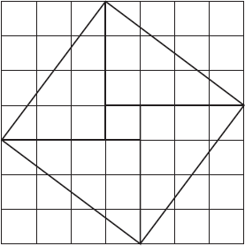
The history of this theorem is long and convoluted. It may or may not have been proven by Pythagoras of Samos (circa 500 BCE); it is a highlight of the first book of Euclid’s Elements; and it certainly was known in ancient China. In fact, Figure 1 appears in Arithmetic Classic of the Gnomon and the Circular Paths of Heaven (China, circa 600 BCE). The accompanying argument is written using the specific values of 3, 4, and 5, but it is easy to use modern notation and convert this ancient argument-by-example into what would be accepted as a modern mathematical proof.
A PROOF OF THE PYTHAGOREAN THEOREM. Let be a right triangle, with sides of length a, b, and c, where for convenience1 we have  . Then you can arrange four copies of as in Figure 1, where the right angles are in the interior of the figure, and the four hypotenuses form a bounding quadrilateral. Call this quadrilateral
  , since it has our sides.
Because the sum of the interior angles in any triangle is 180 , the sum of the two non-right angles of is 90. At each corner of the boundary quadrilateral there is a copy of each of these non-right interior angles, hence at each corner of there is a right angle. Thus is a rectangle. Furthermore, each side of comes from the hypotenuse of a copy of , so is a rectangle with four congruent sides, hence is a square. The area of is then
  . Thinking of as being composed of four triangles and a smaller interior square, we know the area of can also be expressed as
 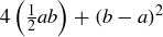 . This implies
Notice, however, that we have not yet established the full Pythagorean Theorem. This argument shows only half of it: that the lengths of the three sides of a right triangle have a certain arithmetic property. The other fact claimed in the Pythagorean Theorem, the other half of the “if and only if” statement, is equally important: triangles with this arithmetic property are right triangles. This fact was used by the ancient Egyptians in surveying and construction, and it is still used by carpenters to construct right angles.
To prove the other direction, assume we have a triangle where  . Let
. Let  be a right triangle with sides a and b and hypotenuse h. By the argument above we know
  , so
, so  . Thus and
  are congruent, and therefore is a right triangle.

You do not need to write multiple proofs to establish the validity of a mathematical theorem. But multiple proofs can provide additional insights, and there are many fun and insightful proofs of the Pythagorean Theorem. In the following example and exercise, we are proving only that the sides of right triangles satisfy the arithmetic condition.
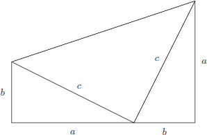
President James Garfield constructed a proof of the Pythagorean Theorem, long before he became President of the United States. His argument begins by forming a trapezoid using two copies of a right triangle, arranged so that side a of one copy and side b of the other copy lie on a line, as in Figure 2.
Exercise 11.1 Verify that Garfield’s trapezoid is composed of three right triangles. Then establish the arithmetic identity  by comparing the area formula for a trapezoid with the sum of the areas of the three triangles that comprise Garfield’s trapezoid.
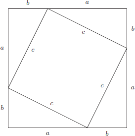
Exercise 11.2 Figure 3 is commonly used in proving the Pythagorean Theorem. Use this figure as inspiration to construct yet another proof of the Pythagorean Theorem.
Exercise 11.3 Find one additional proof of the Pythagorean Theorem, so that you will have seen at least four proofs of this result. You can try to find this proof on your own, but we are really only asking you to consult available resources and read a fourth proof. Which of these proofs do you think give the most insight into why the theorem is true? Explain!
Exercise 11.4 Let A, B, and C be the three vertices of a triangle Δ, where the side opposite to A is a, the side opposite to B is b, and the side opposite to C is c. If the angle at C is less than 90, what can you conclude, if anything, about the two values  and ? Why? What if the angle at C is greater than 90?
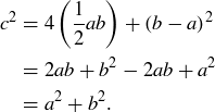
Exercise 11.5 Let  , and z be three positive real numbers, and let Δ be the tetrahedron in
  formed by the points
Because one corner of Δ corresponds to a corner of an octant in  , Δ is a three-dimensional analogue of a right triangle. In fact, a Pythagorean-style formula holds, connecting the areas of the four faces of Δ. Let A, B, and C be the areas of the faces that touch the origin, and let D be the area of the triangle formed by the points X, Y, and Z. Prove that
![]()
Chomp is a game that is easy to describe and play, and which is amenable to mathematical analysis. You should be able to work on this project after having worked through the first two chapters of this book. One of the questions makes use of a result from Chapter 4, but it is not an essential question that is necessary for the successful completion of this project. Chomp appears in Exercise 3.86, which is a nice problem, but not one that is necessary for this project.
Chomp is a fun game for two players, who we’ll call Alice and Bob. They start with an  rectangular “cake,” such as the
  cake shown in Figure 4.
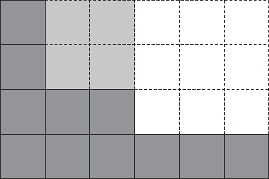
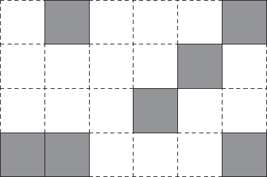
Figure 4. Two plays into the game Chomp. The nine unshaded squares were eaten first; the four lightly shaded squares were eaten second.
The players alternate turns, with Alice going first. On a turn, the player takes a right-angled “bite” from the northeast: a square is removed along with all other squares to the north and east and anywhere in between these directions. In Figure 4 the darkest shading shows the cake remaining after Alice first takes a bite (no shading), followed by a bite by Bob (lighter shading).
The loser of this game is the person who is forced to take the last bite. In the mathematical study of two player strategy games, here’s an important question: If both players use optimal strategy, who wins?
Exercise 11.6 Play Chomp with a friend on boards of varying sizes, such as  ,
,  ,
,  , and
, and  . Play several games of each size, and let each player be Alice half of the time. Make conjectures about which board sizes favor Alice, and which favor Bob. Are there certain boards that you think are guaranteed wins for Alice if she plays optimally? Guaranteed wins for Bob?
Exercise 11.7 Prove that Alice has a winning strategy for any  or
or  board, when
  .
.
Exercise 11.8 For this exercise you should focus on the case of a  game of Chomp. Label each of the six squares with an “A” or a “B” depending on who has a winning strategy if Alice’s first bite is based at that square. We have begun this process in Figure 5. Verify that our two labels are correct, and then label the remaining four squares.

Figure 5. Beginning to label a  game of Chomp. The “A” indicates that if Alice bites this position, then she has a winning strategy. The “B” indicates that if Alice bites in this position, then Bob has a winning strategy.
Exercise 11.9 Prove that, for any  board, Alice has a winning strategy so long as
  . One way to do this is via a proof by contradiction, starting with the assumption that Bob has a winning strategy, and then showing that Alice could always make use of that strategy herself.
Exercise 11.10 Here’s a related game called the Divisor Game, and you will need the Fundamental Theorem of Arithmetic (Theorem 4.11) in order to fully analyze this game. Alice and Bob start with a natural number n. They alternate turns in which a player calls out a natural number that divides n, with the following restriction: each number called out must divide n, but it can’t be a multiple of any number that has already been called out. The loser is the person forced to say 1.
Here’s an example game for  :
:
Alice starts by saying 10; then Bob says 2; then Alice says 15; then Bob says 3; then Alice says 5; and then Bob is forced to say 1. Alice wins!
Who wins for  ? For
? For  ? For any n?
The game of Chomp can be generalized in many ways. One generalization is to remove the assumption that you start with a rectangular cake, so that you allow Alice and Bob to play Chomp on a cake of any shape made up of n  squares in the square lattice. An example of the sort of cake we are allowing is shown in Figure 6. As in the original version, a bite removes some remaining square and all other squares in the northeast quadrant from it, and the player forced to remove the last square loses. In Figure 6, Alice can win by eating the square adjacent to the southwest corner square on her first turn.
Exercise 11.11 Consider the  case and the
  case.
case.
(a) When  , Alice has two choices of which square to eat, and she does not want to eat a square that would remove both squares, as then Bob would win. By examining the possible configurations of two squares, show that Alice always has a choice that will leave one remaining square, meaning that Alice has a winning strategy.
(b) Create a configuration for  where Alice has a winning strategy and a different configuration for where Bob has a winning strategy.
In this more general situation we cannot give a simple statement of which player has a winning strategy. We do, however, know that one of them does have a winning strategy.
THEOREM 11.2. For any  and any cake made up of n squares in the square lattice, one of the two players has a winning strategy for the game of Chomp beginning with that configuration.
This is an example of a more general result about certain types of two-player games: you may not know who has the winning strategy, but you know that someone does!
Exercise 11.12 Here we outline a proof by induction for Theorem 11.2. Start by establishing the base case when  .
.
For the inductive step, assume that for any value of k such that  , someone has a winning strategy for each possible cake shape made up of k little
  squares.
Now, consider Alice eating first from a cake made up of  little squares. Since after any bite she makes there will be no more than n little squares left, by the inductive assumption we know that either Alice or Bob has a winning strategy for the cake that remains after her first bite. Use this insight to prove that either Alice or Bob must have a winning strategy for the original cake.
GOING BEYOND THIS BOOK. If you would like to know more about Chomp, or the mathematics underlying many other games, we recommend Winning Ways for Your Mathematical Plays by Berlekamp, Conway, and Guy [BCG01]. Over the years there have been different editions and volumes of this work – we have listed some in the bibliography – and they are all excellent.
The arithmetic–geometric mean inequality is a fundamental result in analysis. The two-variable version was stated in Exercise 1.1: If a and b are two non-negative real numbers, then
![]()
In this project we will guide you through a proof of this result as well as its natural generalization to any finite number of non-negative real numbers. The argument is a somewhat complicated application of mathematical induction, and so we recommend having worked though Chapters 1 and 2 before beginning this project.
There are a number of ways to compute an average for a given a set of positive numbers,  . The most common method is to add them up and divide:
![]()
This is the arithmetic mean of  . Another approach is to multiply and then take a root:
![]()
This is the geometric mean. We note that the arithmetic mean can easily be applied to a mix of positive and negative numbers, while the geometric mean cannot. Hence for the remainder of this project we will be limiting ourselves to non-negative real numbers.
Exercise 11.13 Gather five or more friends. Give each of them n randomly chosen, non-negative real numbers, where n is some integer greater than 2. Your friends’ job is to compute the arithmetic and geometric means of the numbers you gave them. We will wager that in all cases  . If you can’t find five friends willing to help you with these computations, perhaps you could have a computer assist you in collecting evidence.
You should have found that the arithmetic means were always at least as large as the geometric means of your random sets of real numbers chosen for Exercise 11.13, and that the arithmetic mean was usually strictly larger than the geometric mean. The arithmetic–geometric mean inequality says that the results of Exercise 11.13 were not random. If you didn’t get such results, some of your friends probably need a refresher course on arithmetic.
The second statement, that the inequality is strict, means that
![]()
whenever there is an  that is not equal to some
  in
in  .
.
You will establish the arithmetic–geometric mean inequality via two lemmas.
LEMMA 11.4. Inequality 11.1 holds for all  ,
,  . Further, when
  the inequality is strict whenever
  for some
  .
.
The proof of Lemma 11.4 is by induction on the exponent k.
Exercise 11.14 Begin by establishing the base case, when  , of the inequality. Note that in this case
  and
and  for some
  . Explain why it suffices to establish
![]()
for all  . And then use algebra to show that this is equivalent to showing that
![]()
Since squares of real numbers are non-negative, the result follows.
Exercise 11.15 Explain how the second claim, that the inequality is usually strict, follows from the fact that when  ,
,  .
.
For the inductive step, assume the inequality holds for up to some  , and let
  . We need to establish for any list of
  non-negative real numbers, the inequality
![]()
holds.
Exercise 11.16 Define  and more generally,
  . Since each
  , our induction hypothesis says
![]()
Use the induction hypothesis and the fact that  to establish the inequality.
Exercise 11.17 Prove that the inequality will be strict should  for some .
The second lemma in the proof of Theorem 11.3 works backwards, and can be used to fill in the gaps between  and
and  .
.
LEMMA 11.5. If Inequality 11.1 holds for a natural number n, then it also holds for  .
.
Exercise 11.18 We want to show that the inequality holds for a list of non-negative numbers  to
to  , assuming it holds for lists with one additional number. Define
![]()
the arithmetic mean of the original list of numbers. Then start from the assumption that
![]()
to establish Inequality 11.1 for the original list of  non-negative real numbers.
Exercise 11.19 Verify that you continue to get a strict inequality as long as some .
We can now establish the arithmetic–geometric mean inequality.
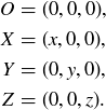
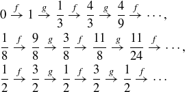
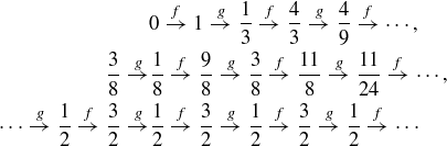
PROOF OF THEOREM 11.3. Given any there is a such that  . Lemma 11.4 shows that Inequality 11.1 holds for lists of length ; Lemma 11.5 then shows that the inequality holds for lists of length n. See Figure 7.
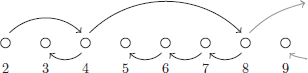
Figure 7. The structure of the proof of the arithmetic–geometric mean inequality. The arrows pointing right are applications of Lemma 11.4, while the ones pointing left are Lemma 11.5.
GOING BEYOND THIS BOOK. This proof of the arithmetic–geometric mean inequality is essentially due to Augustin Cauchy. Our presentation in this project is heavily inspired by An Introduction to Inequalities by Beckenbach and Bellman [BB61]. If this section strikes you as interesting, we strongly recommend you take a look at that book.
This project introduces the complex numbers,  , and focuses on the Gaussian integers,
  . Anyone who has worked through the first four chapters should be able to work on this project. We do use some of the language of functions, which is covered in Chapter 5, but our use of this language is minimal and we expect that it is not necessary to have completed Chapter 5 before taking up this project.
The complex numbers are formed by adding  to the real numbers. Every element of can be expressed as
  , where
  . Addition, subtraction, and multiplication in are defined keeping in mind that
  and
and  . Thus
![]()
The conjugate of a complex number changes the sign of the coefficient of  . That is, the conjugate of is
  .2 Conjugation helps explain division by non-zero complex numbers. In general, as long as
  ,
,
![]()
For example,
![]()
The complex numbers are usually represented by points in the plane, where corresponds to the point  . The distance from the origin to
  is
is  , and so the product of with its conjugate
  is the square of the distance to the origin. As we shall see, this norm
![]()
is a very useful function from to  .
.
Exercise 11.20 The Gaussian integersare the subset of the complex numbers consisting of all integer combinations of 1 and . That is,
![]()
Show that the Gaussian integers are closed under addition, subtraction, and multiplication.
Exercise 11.21 If  , we say α divides β if there is a
  with
with  . As you might expect, we denote this
  , and when α does not divide β we write
  .
.
(a) Show that  .
.
(b) Show that the only divisors of  are
are  , and
, and  .
.
(c) Show that  , and conclude that
  does not deserve to be called a prime number (in the context of Gaussian integers).
Exercise 11.22 Let  be the norm described above.
(a) Prove that, for every α and  ,
,  .
.
(b) Show that the restriction of the norm to produces a function from to  .
.
(c) Is there any  where
where  ?
?
(d) There are 12 Gaussian integers whose norm is 25. Find them, and plot them in the complex plane.
The Gaussian integers seem like a reasonable analog of the integers, just with the addition of the element . It is reasonable to see if Gaussian integers have similar divisibility properties, including unique factorization.
As a cautionary example, we note that
![]()
which might temper your hopes for unique factorization. The situation might seem less severe if one were to notice:
![]()
Thus the two expressions given above for  are connected by
![]()
Define the units of to be those elements  where
where  for some
  .
.
Exercise 11.23 Use the norm to show that if α is a unit in  , then
  . After establishing this lemma, verify that the units of are
  .
.
The norm can help in finding factorizations. For example,  . Since
  , there is a chance that
  where
where  and
and  . In fact,
![]()
Exercise 11.24 Use the norm to assist you with the following questions.
(a) Find a factorization of  where neither factor is a unit.
(b) Show that if  , then either α or β must be a unit.
(c) Just to keep your enthusiasm in check, verify that  divides
  but
but 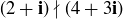 in .
in .
We are now ready to define the notion of a prime number for the Gaussian integers.
Exercise 11.25 Determine if the following Gaussian integers are prime or not. They are arranged in order of increasing norm. While there are quite a few of them, you will gain some critical familiarity with by checking them all.
(a) 
(b) 2
(c) 
(d) 
(e) 3
(f) 
(g) 
And, given your work above, you should now be able to do the following quite quickly.
(h) Prove that if  is a prime number in , then α is a prime in .
(i) Show by example that there are integers that are prime in which are not prime in .
Exercise 11.26 Prove that every Gaussian integer is a Gaussian prime or can be expressed as a product of Gaussian primes. We recommend a proof by strong induction where you induct on the norm of the Gaussian integer.
Exercise 11.27 At this point we have finished guiding you! Review the proof of unique factorization of the integers, and following that general approach, you should now be able to state and prove an analogous result for the Gaussian integers. We aren’t saying this will be easy; we are merely claiming that we have great confidence in your mathematical abilities.
GOING BEYOND THIS BOOK. If you would like to know more about the Gaussian integers and similar number systems, you should read On Quaternions and Octonions [CS03].
Exercise 1.36 asks you to prove that there are arbitrarily large gaps between consecutive primes in , so it is impossible for someone to walk from 0 to infinity along the real line, where the steps are of bounded length and the person is only allowed to step on prime integers. A currently unsolved problem asks the same question in the context of the Gaussian integers, thought of as lattice points in the plane. Namely, is it possible for someone to walk from  to infinity when the steps are of bounded length and the person must only step on points where
  is a Gaussian prime? Figure 8 displays Gaussian primes near the origin. You can read more about this problem in [GWW98], [Loh07], and the references cited by these papers.
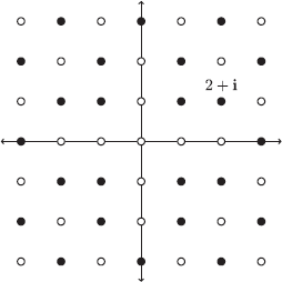
Figure 8. The Gaussian integers inside of the complex plane. The filled circles correspond to the Gaussian primes.
In this project we explore …
THE PIGEONHOLE PRINCIPLE (Lemma 5.21). Let  , where A and B are finite, non-empty sets. If
  , then f is not injective.
We proved this result at the end of Section 5.5. Here we take up some of its consequences and ask you to state and prove a generalized Pigeonhole Principle. We expect that to be successful in this project you will need to have finished the first three chapters and Chapter 5, through the proof of the Pigeonhole Principle in Section 5.5. It will be even easier if in fact you have worked through all of Chapter 5.
11.5.1. Lots of Pigeons! The Pigeonhole Principle can be generalized. For example, if you have 25 pigeons fly into 12 coops, it is certainly the case that at least one coop has more than one pigeon. In fact, it must be the case that at least one coop has more than two pigeons.
Exercise 11.28 In this exercise you will discover and prove a generalization of the Pigeonhole Principle.
(a) Let A and B be two finite sets, with  . How large must A be to ensure that given any
  there is some
  where at least three elements of A are mapped to b?
(b) Let A and B be two finite sets, with  . How large must A be to ensure that given any there is some
  where at least k elements of A are mapped to b?
(c) State a conjectured generalization of the Pigeonhole Principle.
(d) Prove your conjecture.
11.5.2. Pigeonhole Projects. The exercises in this subsection are independent of each other, so you may pick and choose those you find most interesting. Their diversity illustrates the broad applicability of the Pigeonhole Principle, and each is written in a manner that requires you to do some creative exploration of the application. Our recommendation is that you write up a presentation and proof of your generalized Pigeonhole Principle, and illustrate this result by presenting your work on one of the following exercises.
Exercise 11.29 Define a rectangular game board to be an rectangle, with  and both at least 2, which is divided into colored unit squares. A standard chessboard is one example; another example is shown in Figure 9.
(a) A  board is divided into 21 unit squares, each colored black or white. Prove that there must be a rectangular game board contained in this board whose four corner squares all have the same color.
(b) Find examples that illustrate that the claim in part (a) is not true on a  game board for any
  .
.
(c) Find another example that illustrates that the claim in part (a) is not always true for  game boards.
(d) Consider  game boards where the squares can be colored by three different colors. Can you find values of m and n that guarantee there is a game board contained in the board where all four corners have the same color?
(e) Can you state and prove a result that works for c colors, where c is an integer that is greater than or equal to 2?
(f) How might you frame questions like these for rectangular bricks which have been divided into unit cubes? What sort of results can you find in this context?
Figure 9. A  game board colored by two colors. The thick boundaries highlight a game board, and a
  game board, where in each case the four corners have the same coloring.
Exercise 11.30 The positive difference of a pair of distinct integers  is
is  . In this exercise you will consider subsets
  and prove results about the positive differences of pairs chosen from S. You may assume that the number of pairs of elements contained in a set with k elements is
  . More information about this and related formulas is presented in Section 3.8.
(a) Consider subsets  . Prove that if
  , then there are at least two pairs of elements in S with the same positive difference.
(b) Give an example that shows the claim in (a) is false if  .
.
(c) Consider subsets  . Find a value of k such that when
  , then there are at least two pairs of elements in S with the same positive difference.
(d) Conjecture a result along the lines of
Here you should give an explicit formula for f in terms of the variable n. And of course you should prove that your conjecture is correct.
(e) How might you extend your ideas to the situation where S is sufficiently large as to guarantee that there are at least three pairs of elements in S with the same positive difference?
Exercise 11.31 A lattice point in  is any point
  where x and y are both integers.
(a) Prove that if five lattice points are chosen in the plane, then there must be a pair where the midpoint between them is itself a lattice point.
(b) How many lattice points must you choose to guarantee that there are two pairs where the midpoint between each pair is itself a lattice point.
(c) State and prove a result about the number of lattice points that will guarantee that there are n pairs where the midpoint between each pair is a lattice point.
(d) Extend your ideas to lattice points in .
Exercise 11.32 In this problem you will explore the clustering of points chosen inside of a unit square.
(a) Prove that given any 9 points in the unit square, there must be three that are contained in a circle of radius  .
.
(b) Prove that given any 19 points in the unit square, there must be three that are contained in a circle of radius  .
.
(c) Prove that given any 28 points in the unit square, there must be four that are contained in a circle of radius .
(d) Conjecture a result along the lines of the previous parts of this exercise, and prove that your conjecture is correct.
(e) Conjecture a result along the lines of
![]()
Here you should give an explicit formula for f in terms of the variable n. And of course you should prove that your conjecture is correct.
GOING BEYOND THIS BOOK. Like any fundamental result in mathematics, the history of the Pigeonhole Principle is fascinating and complicated. If you are interested in this history, we recommend the article by Rittaud and Heeffer [RH14] as a good entry point to the literature.
Mirsky’s Theorem is a general result about partially ordered sets, so you should have completed Section 6.2 before working on this project, including the definition and exercises on chains and maximal chains in the end-of-chapter exercises for Chapter 6.
Consider the following sequence of nine integers:
![]()
By focusing on particular entries, you can find subsequences that are increasing like the bold entries in
![]()
and subsequences that are decreasing like the bold entries in
![]()
Call such a subsequence a monotone subsequence. We designed our sequence of nine numbers so that the longest monotone subsequences have three terms.
Exercise 11.33 Verify that our sequence contains no monotone subsequences with four terms.
Something interesting happens when a tenth integer is added into this sequence. We randomly selected a new integer and inserted it into a random location in our original sequence to produce
![]()
This sequence now contains monotone subsequences with four terms, for example,
![]()
and
![]()
Exercise 11.34 Do some experimenting to see the emergence of a monotone subsequence with four terms was an accident or if it might be an example of a larger pattern.
(a) Find your own additional integer and insert it into the sequence
![]()
at a random location. Can you find a monotone subsequence with four terms contained in your new sequence?
(b) Repeat part (a).
(c) Repeat part (a) again.
It is a fact that any sequence of ten distinct integers will have a monotone subsequence with four (or possibly more) terms. This is a special case, an example really, of a result first proved by Erdös and Szekeres in the 1930s. After we explore Mirsky’s Theorem, we will return to the Erdös–Szekeres Theorem and use Mirsky’s Theorem to prove it.
Mirsky’s Theorem connects the height of a poset to its antichains. Let  be a partially ordered set. An antichain is a subset of S where no two elements are comparable. For example, if
 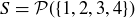 is ordered by containment, then
![]()
is an antichain.
Exercise 11.35 In this problem we will continue to work with the poset of subsets of  ordered by containment.
(a) The poset of subsets of  , ordered by containment, contains 168 antichains. Find five of them.
(b) The largest antichains in the poset of subsets of contain six elements. Find such an antichain.
(c) Find another antichain with six elements, or prove that the antichain with six elements is unique.
A maximal antichain is one that is not properly contained in any other antichain.
Exercise 11.36 For , let  be a zigzag poset with n elements. Find a formula for the size of the largest antichain in
  , and prove that your formula is correct. (Zigzag posets are defined in Exercise 6.49.)
DEFINITION 11.7. An antichain cover of a poset is a collection of antichains, whose union contains all the elements of the partially ordered set. If the antichain cover consists of the antichains 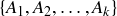 , then the cover has size k.
Exercise 11.37 The following questions provide a bit of practice with antichain covers, in the context of the poset of subsets of 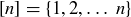 ordered by containment.
(a) Prove that for any fixed integer k,  , the collection of k-element subsets is a maximal antichain.
(b) Prove that the poset  can be covered by
  antichains.
THEOREM 11.8 (Mirsky’s Theorem). Let S be a finite set, partially ordered by  . Then the height of the poset
  equals the size of a minimal antichain cover of S.
Below we outline two approaches to proving Mirsky’s Theorem. The first proof connects the height directly to antichains, and the second is a proof by induction.
Exercise 11.38 Let be a finite poset.
(a) Prove that the intersection of any antichain with a chain can contain at most one element.
(b) Prove that if the height of is H, then any antichain cover must contain at least H antichains.
Exercise 11.39 Let  be a finite poset, and define the height of an element
  to be the maximum number of terms that occur in any chain with s as its largest element. These heights give us a function
  , where
  is the height of the element s.
(a) If H is the height of the poset , prove that h gives a surjection onto 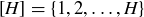 .
.
(b) Prove that if  , then
  is an antichain.
(c) Prove there is an antichain cover of consisting of H antichains.
Exercises 11.38 and 11.39 immediately imply Mirsky’s Theorem:
PROOF OF MIRSKY’S THEOREM. Let be a finite poset of height H, where a minimal antichain cover of contains A antichains. Then Exercise 11.38 shows that  , and Exercise 11.39 shows that
  . Thus
  .
.
Mirsky’s Theorem can also be proven by induction on the height of the poset.
Exercise 11.40 When you complete the following steps you will have outlined an inductive proof for Mirsky’s Theorem.
(a) Base Case: Prove that Mirsky’s Theorem holds for finite posets of height 1.
(b) Lemma: Prove that the set of all maximal elements of a finite poset forms an antichain.
(c) Lemma: Let M be the set of all maximal elements of the poset . Prove that  is a poset whose height is smaller than the height of .
(d) Use the two lemmas above to establish the inductive step.
Having proven Mirsky’s Theorem (twice!), we are now able to head toward a proof of the Erdös–Szekeres Theorem.
COROLLARY 11.9. Let m and n be natural numbers. Then in any partially ordered set with  or more elements, there is a chain with
  elements or an antichain with elements.
PROOF. Using the argument from Exercise 11.39 we see that if the height of the poset is less than then there is an antichain cover consisting of fewer than  antichains, where no two antichains overlap. Denote these antichains by
 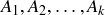 (
( ). Thus
  , and so
![]()
Thus  , and so there must be an antichain with at least elements.
Exercise 11.41 Use Corollary 11.9 to prove the Erdös–Szekeres Theorem: Each sequence of  distinct real numbers possesses a monotone subsequence with terms. As a hint, define an ordering on the terms of the sequence by saying
  if
if  and
and  .
.
For a graphical interpretation of this result, see Figure 10.
Figure 10. Mirsky’s Theorem guarantees that you can find an increasing or decreasing constellation of length in the graph of a sequence with distinct terms.
Exercise 11.42 In Exercise 6.8 we described a partial ordering on closed and bounded intervals  . Use Mirsky’s Theorem to prove that for any collection of
  closed and bounded intervals there must be either that are disjoint or that share a common point.
GOING BEYOND THIS BOOK. Mirsky first published his now eponymous theorem in [Mir71]. That paper is quite readable and is recommended, particularly for the way it discusses the connection between the result presented in this project and a related result, Dilworth’s Theorem. The original paper by Erdös and Szekeres [ES35] is also worth reading, particularly with an eye toward how these ideas have evolved over the decades since their first presentation.
We have seen that knowing the order of an Abelian group can be useful. It is immediate that  , but the order of
  is less clear. Since the elements of correspond to the integers k where
  and
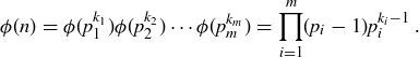
and  , we are simply wondering how many natural numbers less than or equal to m are relatively prime to m. The function
![]()
is known as Euler’s totient function. Our goal in this section is to find a nice formula for ϕ. As part of the motivation for studying ϕ comes from the units arising in modular arithmetic, this project is appropriate for students who have worked through Section 6.6.
Exercise 11.43 Explain why  for all primes p.
Here’s one that is a bit more difficult.
Exercise 11.44 Prove that if p is prime, then  .
.
For example, if you are considering  then
then
![]()
We do need to verify that this remainder map is well defined.3 To do this, consider any integer b where  . Thus
 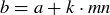 . So
. So
![]()
Thus our definition does not depend on the representative used in computing the answer.
We now get to play with this remainder map. Let’s first look at  .
.
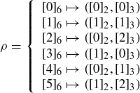
The remainder map has given us a bijection between the six elements in  and the six elements in
  . Before we make any hasty conjectures, let’s look at another example, this time considering
  :
:
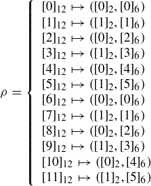
In this case we do not get a bijection. As always, this ought just to make us more curious …
PROOF. Since  , it suffices to show that ρ is injective.
If  , then n and m divide
  . Hence the least common multiple of m and n divides
  (see Exercise 4.42). Because m and n are relatively prime,
  divides . So
  .
.
Exercise 11.45 Show that the remainder map gives a bijection:
![]()
when m and n are relatively prime.
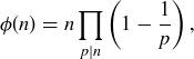
Exercise 11.46 Let the prime decomposition of n be  , with each
  . Prove that
At this point we have an effective method for computing Euler’s totient function. For example,  .
.
Finally, we are in a position to present an alternate formula for ϕ that is often preferable:
THEOREM 11.12. Let . Euler’s totient function ϕ is given by
where  stands for the set of primes p that divide n.
For example,
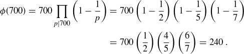
Exercise 11.48 Prove Theorem 11.12.
If you are ambitious, we recommend that you explore bounds on Euler’s totient function in the following exercise.
Exercise 11.49 Figure 11 shows the graph of Euler’s totient function  , up to
  .
.
(a) Prove that this graph is bounded above by the straight line  , as Figure 11 suggests.
(b) Prove that no line of slope  could be an upper bound on the graph of ϕ.
(c) In Figure 11 we have drawn in the line connecting the origin to  . It appears that this line gives a lower bound on ϕ. Show that this is in fact false.
(d) Prove that 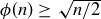 for all integers .
In Section 7.6 we demonstrated the tremendous utility of the Schröder–Bernstein Theorem, but we did not provide a proof of this theorem. The goal of this project is for you to construct a proof, and before working on this project you should review Exercise 7.18.
THEOREM 11.13 (The Schröder–Bernstein Theorem). Let A and B be sets, and assume there are injections and  . Then A and B have the same cardinality.
Every element  determines a sequence of elements, alternating between the sets A and B. The sequence starts with a and then alternately applies f and g:
![]()
It is cleaner to visualize this sequence as the filling in of blanks in the following diagram:
![]()
You can also attempt to build out this sequence to the left, essentially applying the inverse of g and f. However, this is only possible if you are working with elements in the range of g and f, respectively. Thus, while the sequence will continue to the right indefinitely, it may not extend indefinitely to the left.
![]()
We will call these sequences back-and-forth sequences, as they bounce between A and B. When discussing a back-and-forth sequence, we always assume that it has been extended as far as possible to the left.
EXAMPLE 11.14. The Schröder–Bernstein Theorem can be easily applied to show that  . For example, there are injections
  and
and 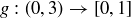 , where
  and
and  . These functions lead to the following sequences:
The top back-and-forth sequence cannot be extended to the left, because the value 0 is not in the range of g. The middle sequence can be extended one step to the left, since  . However,
  , so this sequence extends no further to the left. Finally, it is clear that the bottom sequence extends indefinitely to the left. Thus we have:
Exercise 11.50 Let and  be injections. Define a relation ~ on the elements of A by saying
  when a and
  are both in a shared back-and-forth sequence.
(a) Prove that ~ is an equivalence relation, and therefore the equivalence classes partition A.
(b) State and prove the same result for the elements of B.
DEFINITION 11.15. A back-and-forth sequence that extends indefinitely to the left is a bi-infinite sequence. Those that cannot be extended indefinitely to the left are called A-sequences or B-sequences, depending on whether the left-most element is in A or B.
Exercise 11.51 This exercise refers back to the situation described in Example 11.14.
(a) Show that there are only two A-sequences for this example.
(b) Show that there are infinitely many B-sequences.
Exercise 11.52 Let and  be injections.
(a) Prove that f is a bijection when restricted to the elements occurring in an A-sequence.
(b) Prove that  is a bijection when restricted to the elements occurring in a B-sequence.
(c) Prove that f and  are both bijections when restricted to the elements in a bi-infinite sequence.
Exercise 11.53 Prove the Schröder–Bernstein Theorem.
Exercise 11.54 Apply your proof of the Schröder–Bernstein Theorem to construct an explicit bijection between  and
and  .
.
Exercise 11.55 Show that the bijection h given in Exercise 7.18 comes directly from the injections f and g discussed earlier in Section 7.6.
This project is in fact two projects. We begin with an elementary discussion of Cauchy sequences. The first sub-project proves that a real-valued sequence is Cauchy if and only if it converges. The second sub-project, which can be done independently of the first, outlines the construction of the real numbers via Cauchy sequences of rational numbers. We make frequent use of material in Chapter 8, up to and including Section 8.5, throughout this project.
DEFINITION 11.16. A sequence  of real numbers is a Cauchy sequence if, given any real number
  , there is an
  such that
![]()
whenever m and n are both greater than N.
The first exercise provides a good test case for practicing with this definition.
Exercise 11.56 Let  be a decimal expansion of some real number r. Here
  and each
  . For each define
![]()
Prove that the sequence of rational numbers  is a Cauchy sequence.
Exercise 11.57 Construct an example of a Cauchy sequence that is not monotone.
11.9.1. Real-valued Cauchy Sequences. The goal of this sub-project is to prove that a real-valued sequence  converges if and only if it is Cauchy.
Exercise 11.58 Let be a real-valued Cauchy sequence. Because is a Cauchy sequence, by its definition there is an  such that
  for all m and n greater than N. Consider then the set of initial terms
  and the set of values that appear in the tail
  .
.
(a) Explain why the set of initial terms,  , is bounded.
(b) Show that the terms in the tail,  , are all contained in the closed interval
  .
.
(c) Combine the facts above to prove that Cauchy sequences are bounded.
Because Cauchy sequences are bounded, given a Cauchy sequence  we may define an associated sequence of upper bounds
  . We let
  be any upper bound for all the terms in . We define
  to be the average of
  and , if this average is an upper bound for
  , and otherwise we set
  . And in general
![]()
This sequence of upper bounds is illustrated in Figure 12, where the original Cauchy sequence is graphed using black circles, and the associated sequence of upper bounds (with chosen to be 4) is displayed with crosses. The figure indicates, correctly, that both sequences converge to a limiting value of 2.
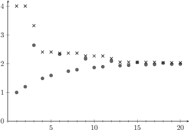
Figure 12. A Cauchy sequence is shown with black circles, and an associated sequence of upper bounds is displayed with crosses.
Exercise 11.59 Let  be a Cauchy sequence and let
  be any upper bound on the set of terms
  .
.
(a) Prove that the associated sequence of upper bounds  defined as above is a bounded, monotone decreasing sequence. Conclude that it must converge to some real number μ.
(b) Prove that the Cauchy sequence converges to μ as well.
Exercise 11.59 gives a very important method of demonstrating that a real-valued sequence converges. Constructing a proof of convergence using the original definition requires that you also already know the limit of the sequence. Proving that a sequence is Cauchy, however, requires only an argument that uses the terms of the sequence.
You are now in a position to establish the main result of this subsection. We anticipate that you will want to use the following approach: If converges to a limiting value α, then for any you know that
![]()
This is an application of the triangle inequality:  for all
  .
.
Exercise 11.60 Prove that a real-valued sequence is Cauchy if and only if it converges.
11.9.2. Constructing the Real Numbers. Given the natural numbers,  , you can construct the set of integers, , by adding 0 and defining negative numbers. Given the integers, you can construct the rationals,
  ; one method for doing this is presented in Exercise 6.75. Here we describe a way to construct the real numbers, , from the rationals.
There are various definitions that lead to the real number system, and the following set of axioms is one of the most common. This definition begins by assuming there is a set of elements denoted by , two binary operations  and
and  that map
  to , and a relation
  on . This collection defines the real numbers if it satisfies the following 12 axioms.
(1) For every a, b, and  ,
,  and
and  .
.
(2) For every a and  ,
,  and
and  .
.
(3) For every a, b, and  ,
,  .
.
(4) There is an element called 0 such that  for all
  .
.
(5) Given any  , there is an element such that
  .
.
(6) There is an element called 1 such that  for all .
(7) For every  , there is a such that
  .
.
(8) For every  and , if
  then
then  .
.
(9) For every and , if and  then
then  .
.
(10) For every a and  , exactly one of the following is true:
  ,
,  , or
, or  .
.
(11) For every a and and every  , if then
  .
.
(12) If S is a non-empty subset of that is bounded above, then S has a least upper bound.
Our goal then is to start with the rational numbers, construct a set along with  and , and verify that the axioms above hold. In order to do so, we limit our discussion in this section to rational sequences, that is, sequences
  where every
  . If q is a rational number, we let
  be the constant sequence,
![]()
DEFINITION 11.17. Two Cauchy sequences and  are defined to be equivalent if the sequence of differences
  converges to 0.
Exercise 11.61 Prove that the sequence  and the sequence
  are equivalent Cauchy sequences.
Exercise 11.62 Prove that the “equivalent” relation defined above lives up to its name and is indeed an equivalence relation on the set of Cauchy sequences.
We define to be the set of equivalence classes of rational Cauchy sequences. We define addition and multiplication of rational Cauchy sequences via
![]()
For example,
![]()
Exercise 11.63 Addition and multiplication are defined for specific sequences, not for equivalence classes. And our definition of states the the elements of are not sequences, but rather equivalence classes of sequences. This means you have some work to do! We need to establish that the sum and product of rational, Cauchy sequences are rational Cauchy sequences. We also need to verify that these operations are well defined on equivalence classes.
(a) Prove that if  and
and  are rational Cauchy sequences, then so is
  .
.
(b) Prove that if and  are rational Cauchy sequences, then so is
  .
.
(c) Let  and
and  be equivalent sequences. Prove that
![]()
(d) Let and be equivalent sequences. Prove that
![]()
Exercise 11.64 Verify that the Algebraic Axioms hold, with the constant sequence  functioning as the additive identity 0 and
  functioning as the multiplicative identity 1.
DEFINITION 11.18. For two rational Cauchy sequences and  , define
  if they are not equivalent and if there is an
  such that
  for all
  . We say
  if either the two sequences are equivalent or if
  .
.
Exercise 11.65 We have defined for specific sequences, not on equivalence classes of sequences. We need to verify that makes sense on equivalence classes, and then verify that the order axioms hold.
(a) Let and be equivalent sequences. Prove that
![]()
Thus our definition is well defined on equivalence classes.
(b) Verify that the order axioms hold.
Exercise 11.66 Let S be a set of rational Cauchy sequences which is bounded above. Prove that S has a least upper bound by mimicking the “sequence of upper bounds” approach from the previous subsection. If you are working with representatives from the equivalence classes, be sure to verify that your arguments hold regardless of the chosen representatives.
Finally, having constructed the real numbers, it is a good idea for us to verify that the usual description in terms of decimal expansions is indeed accurate. Define a standard decimal expansion sequence to be a Cauchy sequence of the form discussed in Exercise 11.56, with the added requirement that given any  there is an
  such that
  , so that decimal expansions are not allowed to have a tail of repeating 9s. This final exercise justifies the use of decimal expressions to represent the real numbers.
Exercise 11.67 Prove that every rational Cauchy sequence is equivalent to a standard decimal expansion sequence.
GOING BEYOND THIS BOOK. There are other ways of constructing the real numbers that do not involve equivalence classes of Cauchy sequences. The method of Dedekind cuts is nicely presented in Abbott’s Understanding Analysis [Abb15]. Both the approach via Cauchy sequences and the approach of Dedekind date to the early 1870s. It should be noted, however, that the history of constructions of is complicated, with credit certainly being due to Cantor, Heine, Dedekind, Méray, and Weierstrass (at the least!). Some would also include work of Simon Steven on numbers with unbounded decimal expansions in the 1600s, and perhaps even work of Eudoxus in ancient Greece. While it is not particularly focused on constructions of , Grabiner’s The Origins of Cauchy’s Rigorous Calculus [Gra81] is an excellent history of the development of analysis.
In this project we introduce the Cantor set, a subset of the closed unit interval  that is formed by repeatedly removing open intervals. The Cantor set has a number of interesting and often counterintuitive properties, the most accessible being the fact that it is both a small subset of and a large collection of points in . In this project we assume you have worked through Chapters 7 and 8, or at the least have a good intuition about the real numbers.
The process for defining the Cantor set  begins with the interval
  , and then creates
![]()
The subset  consists of two closed intervals, and we remove the “middle thirds” from both of them to form
  . That is, we remove
  and
and  from to form
  :
:
![]()
The subset consists of four closed intervals. We then remove the middle thirds of each of them to form  , consisting of eight closed intervals, and we continue this process to create a subset
  for each
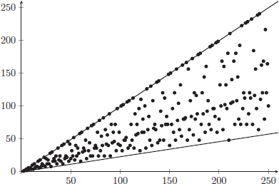
  . The process is visualized in Figure 13.
The Cantor set is the end result of this process; that is, is the set of points in that are never removed in forming any of the sets  .
.
You can also develop the Cantor set using rescaling and translating. If  and , define
![]()
For example, if  then
then  is the interval
  . And, directly related to our discussion of the Cantor set,
![]()
Exercise 11.68 Verify that the next step of forming can be expressed in the same manner:
![]()
Exercise 11.69 Prove that the set is composed of  closed intervals, each of length
  , for a total combined length of
  . Then prove that the open intervals removed in forming the Cantor set are pairwise disjoint and have combined length equal to 1.
Exercise 11.69 indicates that is small, but it is not empty. The numbers 0 and 1 are in every , hence 0 and 1 are elements in the Cantor set . And there are quite a few more points in in addition to these two.
Exercise 11.70 We pointed out that 0 and 1 must be in . Find two other real numbers that are in and explain how you know that they must be in the Cantor set. Then describe an infinite set of real numbers in .
Our discussion of the cardinality of the Cantor set will use the Nested Intervals Property of the real numbers.
THEOREM 11.20 (Nested Intervals Property). Let  be a collection of closed, bounded intervals that are nested; that is,
![]()
Then the intersection of all of these intervals is non-empty:
![]()
Further, if the widths of the intervals decrease to zero, that is
![]()
then the intersection is a set containing a single real number.
Exercise 11.71 Exercise 8.39 asked you to prove the main part of this result: the intersection is non-empty. Please complete this exercise if you haven’t done so already, and then prove that the additional claim that having the widths go to 0 implies that the intersection is a single real number.
In order to apply the Nested Intervals Property to the Cantor set we need a bit of additional notation. The first approximation to the Cantor set, , consists of two intervals,
![]()
We will refer to  as the left interval, which we denote
  , and
, and  as the right interval,
  . Thus
  .
.
In passing to we need to divide into its left and right sub-intervals,  and
and  , and we need to divide into its left and right sub-intervals,
  and
and  . Thus
![]()
Similarly listing the eight intervals that comprise  from left to right, we have
![]()
Define a properly nested sequence of Cantor sub-intervals to be a nested sequence where the first interval comes from , the second from , and so on. One example would be
![]()
Exercise 11.72 Find a one-to-one correspondence between the set of properly nested sequences of Cantor sub-intervals and the Cantor set, and prove that your function is a bijection.
Exercise 11.73 Prove that the Cantor set is uncountable. (We recommend using the idea behind Cantor’s Diagonal Argument, applied to properly nested sequences of Cantor sub-intervals.)
In Exercise 11.69 you showed that the Cantor set is formed by removing open intervals of total length 1, starting from the closed interval . This indicates that must be rather small. Yet in Exercise 11.73 you proved that has the same cardinality as . That is a good stopping place. However, if you feel like pushing forward just a bit more, feel free to work on a final exercise.
Exercise 11.74 If A and B are two sets of real numbers, we can define the sum of A and B as
![]()
For instance, if  and
and  , then
![]()
As another example, if A and B are both equal to the closed interval , then 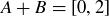 . What’s remarkable is that, despite how small seems to be as a geometric subset of , you can show that
  is equal to the entire closed interval
  as well.
(a) Recall that 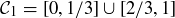 . Thus
  consists of four solid squares in the first quadrant, as shown in Figure 14. Prove that
  consists of those
  such that the line
  intersects . For example, Figure 14 shows that
  .
.
(b) Conclude that  .
.
(c) Use induction to prove that  .
.
(d) Prove that  . Warning: This does not follow immediately from the previous statement!
In Section 10.8 we explored ways you can distinguish some groups of order 12. In this project you will come up with arguments proving that five groups of order 8 are indeed distinct, that is non-isomorphic. It is also the case that these five groups are the only groups of order 8, meaning that any group of order 8 must be isomorphic to one of these five groups. Proving that they are the only groups of order 8 is, however, beyond what we can do given our limited introduction to group theory.
Exercise 11.75 Prove that the three Abelian groups
![]()
are distinct. That is, no two are isomorphic.
Exercise 11.76 Show that the symmetries of a square –  from Section 10.2 – is a non-Abelian group of order 8. What result proves that this group cannot be isomorphic to the three Abelian groups of order 8 in Exercise 11.75?
Let’s look at one more group of order 8, the unit quaternions. Let
![]()
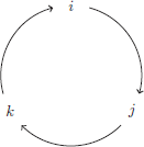
where all products can be determined from the following equalities:  ,
,  ,
, 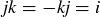 and
and  . These rules can be remembered by using the circle shown in Figure 15: the product of two consecutive elements is the third one, going clockwise. The same is true going counterclockwise, except that you get the negative of the third element.
Exercise 11.77 Make a Cayley table for  , and illustrate via examples that is not Abelian.
Exercise 11.78 If you have had exposure to matrices and matrix multiplication, then you can also view  as a group of eight matrices. As examples, the elements i and j are described by the following
  matrices:
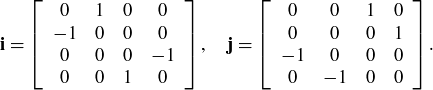
Write down all eight matrices that form .
Exercise 11.79 In order to prove that we now have five non-isomorphic groups of order 8, you need to show that and are not isomorphic. One approach would be to determine how many elements in each group have order 2.
If you would prefer a bigger challenge, where we have not given as many guiding hints, then you might explore groups of order 18 as an alternative to this project. There are five non-isomorphic groups of order 18. Find them, describe them, and prove that it is the case that no two of them are isomorphic.
1 Why is it important for us to say “for convenience” when making this assumption? Why is it also a legitimate step?
2 The conjugate of a complex number α is usually denoted by placing a bar over α, as in  .
.

 is
is  , then exactly one of
 , where both are at least 2. Define the
  by
by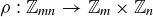
 .
.
 and
and  be as above. Define the set
  to be
to be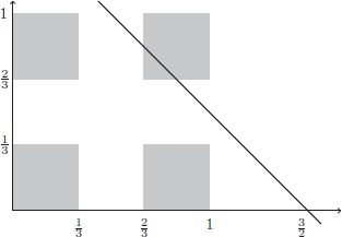
 for Exercise