In recent decades, there has been a substantial increase in the use of personal computers for the purposes of technical analysis. Not surprisingly, this has encouraged many traders and investors to use their own mechanical, or automated, trading systems. These systems can be very helpful as long as they are not adopted as a substitute for judgment and thinking. Throughout this book I have emphasized that technical analysis is an art, the art of interpreting a number of different and reliable scientifically derived indicators. I believe that mechanical trading systems should be used in one of two ways. The preferred method is to incorporate a well thought-out mechanical trading system to alert the trader or investor that a trend reversal has probably taken place. In this method, the mechanical trading system is an important filter, but represents just one more indicator in the overall decision-making process. The other way in which a mechanical trading system can be used is to take action on every signal. If the system is well thought out, it should generate profits over the long term. However, if you pick and choose which signal to follow without other independently based technical criteria, you run the risk of making emotional decisions, thereby losing the principal benefit of the mechanical approach.
Unfortunately, most mechanical trading systems are based on historical data and are constructed from a more or less perfect fit with past, in the expectation that history will be repeated in the future. This expectation will not necessarily be fulfilled because market conditions change. A well thought-out and well-designed mechanical system, however, should do the job reasonably well.
Remember that you are interested in future profits, not perfect historical simulations. If special rules have to be invented to improve results, the chances are that the system will not operate successfully when extrapolated to future market conditions.
One of the great difficulties of putting theory into practice is that a new factor, emotion, enters the scene as soon as money is committed to the market. The following advantages therefore assume that the investor or trader will follow the buy and sell signals consistently:
• A major advantage of a mechanical system is that it automatically decides when to take action; this has the effect of removing emotion and prejudice. The news may be atrocious, but when the system moves into a positive mode, a purchase is automatically made. In a similar vein, when it appears that nothing can stop the market from going through the roof the system will override all possible emotions and biases and quietly take you out.
• Most traders and investors lose in the marketplace because they lack discipline. Mechanical trading requires only one aspect of discipline: the commitment to follow the system.
• A well-defined mechanical system will give greater consistency of profits than a system in which buying and selling decisions are left to the individual.
• A mechanical system will let profits run in the event that there is a strong uptrend, but will automatically limit losses if a whipsaw signal occurs.
• A well-designed model will enable the trader or investor to participate in the direction of every important trend.
The disadvantages of using mechanical systems are as follows:
• No system will work all the time, and there may well be long periods when it will fail to work.
• Using past data to predict the future isn’t necessarily a valid approach because the character of the market often changes.
• Most people try to get the best or optimum fit when devising a system, but experience and research tell us that a historical best fit doesn’t usually translate into the future.
• Random events can easily jeopardize a badly conceived system. A classic example occurred in Hong Kong during the 1987 crash, when the market was closed for 7 days. There would have been no opportunity to get out, even if a sell signal had been triggered. True, this was an unusual event, but it’s surprising how often special situations upset the best rules.
• Most successful mechanical systems are trend-following by nature. However, there are often extended periods during which markets are in a nontrending mode, which renders the system unprofitable.
• “Back-testing” won’t necessarily simulate what actually would have happened. It is not always possible to get an execution at the price indicated by the system because of illiquidity, failure of your broker to execute orders on time, and so forth.
A well-designed system should try to capitalize on the advantages of the mechanical approach, but should also be designed to overcome some of the pitfalls and disadvantages already discussed. In this respect, there are eight important rules that should be followed:
• Back-test over a sufficiently long period with several markets or stocks. The more data that can be tested, the more reliable the future results are likely to be.
• Evaluate performance by extrapolating the results over an earlier period. In this case, the first step would involve the design of a system based on data for a specific time span, such as 1977 to 1985 for the bond market. The next step would be to test the results from 1985 to 1990 to see whether or not your approach would have worked in the subsequent period. In this way, rather than “flying blindly” into the future, the system is given a simulated but thorough testing using actual market data.
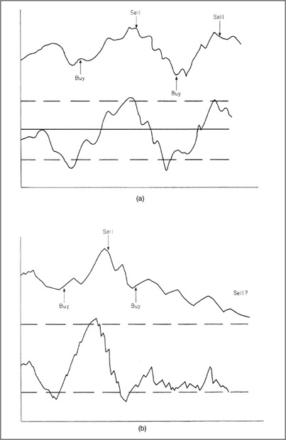
• Define the system precisely. This is important for two reasons. First, if the rules occasionally leave you in doubt about their correct interpretation, some degree of subjectivity will permeate the approach. Second, for every buy signal there should be a sell signal, and vice versa. If a system has been devised using an overbought crossover as a sell and an oversold crossover as a buy, it might work quite well for a time. An example is shown in Figure 34.1a. On the other hand, there could be long periods during which a countervailing signal is not generated, simply because the indicator does not move to these extremes. Failure to define the system precisely can, therefore, result in significant losses, as shown in Figure 34.1b.
FIGURE 34.1 Overbought/Oversold Crossovers

• Make sure that you have enough capital to survive the worst losing streak. When devising a system, it is always a good idea to assume the worst possible scenario and to make sure that you start off with enough capital to survive such a period. In this respect, it is worth noting that the most profitable moves usually occur after a prolonged period of whipsawing.
• Follow every signal without question. If you have confidence in your system, do not second-guess it. Otherwise, unnecessary emotion and undisciplined action will creep back into the decision-making process.
• Use a diversified portfolio. Risks are limited if you place your bets over a number of different markets. If a specific market performs far worse than it ever has in the past, the overall results will not be catastrophic.
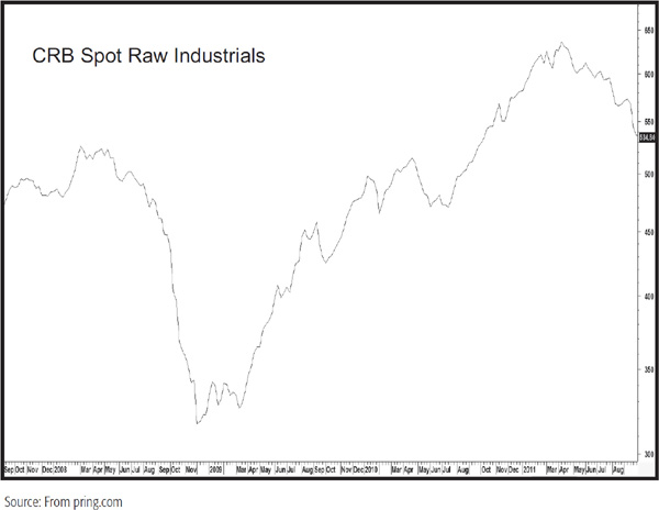
• Trade only markets that show good trending characteristics. Chart 34.1 shows the lumber market between 1985 and 1989.
CHART 34.1 Lumber, 1985–1989

During this period the price fluctuated in a volatile, almost haphazard, fashion and clearly would not have lent itself to a mechanical trend-following system. On the other hand, the Commodity Research Board (CRB) Spot Raw Industrial Materials Index (Chart 34.2) shows an example of both a downtrending and uptrending price trend. Although it is subject to the odd confusing trading range, it has, by and large, moved in consistent trends.
CHART 34.2 CRB Spot Raw Industrials, 2007–2011
• Keep it simple. It is always possible to invent special rules to make back-testing more profitable. Overcome this temptation. Keep the rules simple, few in number, and logical. The results are more likely to be profitable in the future, when profitability counts.
There are basically two types of market conditions: trending and trading range. A trending market, as shown in Figure 34.2, is clearly suitable for moving-average (MA) crossovers and other types of trend-following systems.
FIGURE 34.2 Trade-off Between Timeliness and Sensitivity
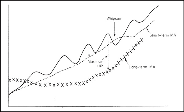
In this kind of situation, it is very important to define the risk since an MA is a trade-off between volatility and sensitivity. In Figure 34.2, the maximum distance between the short-term MA, shown as the dashed line, and the series, shown as the solid line, is the maximum risk. Unfortunately, the short-term MA whips around and gives several false signals. Although the risk of the individual trade defined by the crossover of this MA is small, the chances of unprofitable signals are much greater. On the other hand, a longer-term MA, shown by the X’s, offers larger maximum risk but fewer whipsaws.
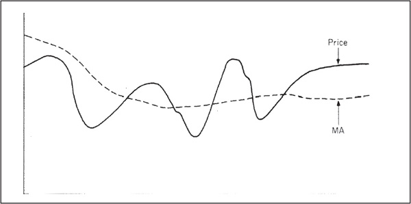
MAs, as shown in Figure 34.3, are virtually useless in a trading range market since they move right through the middle of the price fluctuations and almost always result in unprofitable signals. Oscillators, on the other hand, come into their own in a trading range market. They are continually moving from overbought to oversold extremes, which trigger timely buy and sell signals. During a persistent uptrend or downtrend, the oscillator is of relatively little use because it gives premature buy and sell signals, often taking the trader out at the beginning of a major move. The ideal automated system, therefore, should include a combination of an oscillator and a trend-following indicator.
FIGURE 34.3 MA Crossovers in Trendless Markets
The risk and reward for oscillator-type signals generated from overbought and oversold extremes are shown in diagrammatic form in Figure 34.4.
FIGURE 34.4 Relationship Between Profits and Risk Per Trade Based on Opportunities

The number of potential trading opportunities is represented on the horizontal axis and the risk on the vertical axis. There are very few times when an oscillator is extremely overbought or extremely oversold, but these are the occasions when the profit per trade is at its greatest and the risk the smallest. Moderately overbought conditions are much more plentiful, but the profits are lower and the risk higher. Taken to the final extreme, slightly overbought or oversold conditions are extremely plentiful, but the risk per trade is much higher and profits are significantly lower. Ideally, a mechanical trading system should be designed to take advantage of a situation in which profits per trade are high and risk is low. Execution of a good system, therefore, requires some degree of patience because these types of opportunities are limited.
Turning points in price trends are often preceded by a divergence in the oscillator, so it is a good idea to combine signals from extreme oscillator readings with some kind of MA crossover. This won’t result in a perfect indicator, but it might help to filter out some of the whipsaws.
When the simulated results of a mechanical system are being reviewed, there is a natural tendency to look at the bottom line to see which system would have generated the most profits. However, top results do not always indicate the best system. The reasons for this are as follows:
• It is possible that most, or all, of the profit was generated by one signal. If so, this would place lower odds on the system’s generating good profits in the future since it would lack consistency. An example of an inconsistent system is shown in Table 34.1, which represents signals generated by a 10-day MA crossover of an oscillator that was constructed by dividing a 30-day MA by a 40-day MA (a form of moving-average convergence divergence, or MACD). The market being monitored was Hong Kong during the 1987–1988 period. The system would have gained nearly 1,200 points, compared to a buy-hold approach, which would have lost 800 points. However, this excellent gain would have actually resulted in a loss had it not been for the fact that a prescient short-sell signal occurred just before the 1987 crash.
TABLE 34.1 Hang Seng 3-Month Perpetual 30/40 Oscillator Performance, 1987—1988

• Another consideration involves the identification of the worst string of losses (the largest drawdown). After all, it is no good having a system that generates a large profit over the long term if you don’t have sufficient capital to ride out the worst period. There are two things to look for in this respect: the string of losing signals and the maximum amount lost during these adverse periods.
• A system that generates huge profits but requires a significant number of trades is less likely to be successful in the real world than is a system based on a moderate number of trades. This is true because the more trades that are executed, the greater the potential for slippage through illiquidity and so on. More transactions also require more time and involve greater commission costs.
In virtually every situation, the best signals invariably occur in the direction of the main trend. It is easy to pick out the direction of the primary trend in hindsight, of course, but in the real world we have to use some kind of objective approach to determine the direction of the main trend.
One idea might be to calculate a 12-month MA and to use the position of the price relative to the average as a basis for determining the primary trend. The trading system would be based on daily and weekly data and would be acted upon on the long side only when the index was above the average; short signals would be instigated when it was below.
There are two drawbacks to this approach. First, the market itself may be in a long-term trading range in which MA crossovers do not correctly identify the main trend. Second, the first bear market rally quite often occurs while the price is above its 12-month MA. In effect, the buy signal associated with that rally would be operating against the main trend. By and large, though, most markets trend, and this approach will filter out a lot of the countercyclical moves.
An alternative is to use a long-term momentum series, such as the monthly Know Sure Thing (KST), calculated along the lines discussed in Chapter 15. When the KST is rising and the price is above its 12-month MA, a bull market environment is indicated, and all trades would be made from the long side. When the KST is falling and the price is above its 12-month MA, the chances are that the primary trend is in the process of peaking; no positions would be instigated. If you already had some exposure, the topping-out action of the KST would indicate that some profits should be taken, but total liquidation of the position would probably be better achieved at the time of a negative MA crossover. A trade would be activated only when the KST and the price, vis-à-vis its MA, were in a consistent mode. For example, when the KST peaks out and the market itself falls below its 12-month MA, a bear market environment is indicated and only trades on the short side should be initiated. If you do not have access to the KST, the MACD, using an 18/20/9 combination on monthly data, is a close substitute.
A technique that enables investors to take advantage of both trending and trading range markets is to combine an MA and an oscillator in such a way that buy signals are triggered when the oscillator has fallen to a predetermined oversold level and the price itself subsequently crosses above an MA.
The position is liquidated if the price crosses below the MA. On the other hand, if the oscillator crosses to an overbought level prior to an MA crossover, part of the position will be sold in recognition of the possibility that the market might be experiencing a trading range. The other part of the position will continue to ride until an MA sell signal is triggered.
This approach will make it possible to capitalize on the potential of a trending market, but some profits will be taken in case subsequent market action turns out to be part of a volatile trading range.
Recognizing that oscillators often diverge at important market turning points, an alternative might be to wait for it to move to an extreme for a second time before buying on an MA crossover. The same rules as previously described would be used for selling.
Now it is time to take an actual example of a system by combining these two techniques. The security I chose is a continuous contract for U.S. T-bonds, an MA, and a price oscillator, as shown in Chart 34.3. A price oscillator was calculated by dividing a short-term MA by a longer-term one. In this case, I used a one-period MA, that is, the close as the shorter average and the10-day simple MA as the longer-term one. The 10-day average is plotted in the upper panel with the oscillator underneath.
CHART 34.3 Treasury Bonds and a 1/10 Price Oscillator
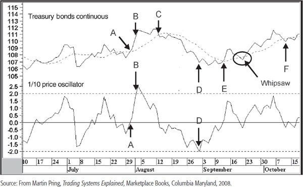
Chart 34.3 shows the way the system works. It is really very simple: Buy when the price crosses above the 10-day MA (as it does in late July at point A). Then sell when it crosses below the average or when the price oscillator reaches a specific predetermined level. The oscillator reaches the designated overbought level a few days later (B). In this case, I selected the +2 and –2 percent. This means the overbought and oversold lines are the equivalent of the price being 2 percent above and below the 10-day MA. Then, in early August, the price crosses below the average and this initiates a short signal (C). The position covered at the end of the month is fairly close to the actual low as the oscillator touches its oversold zone (D). The next buy signal comes on an MA crossover in early September (E). The oscillator never has a chance to move to the +2 percent level because the MA crossover comes first. The next short signal is a whipsaw, followed by the final buy that resulted in a small profit (F).
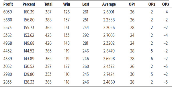
I optimized (optimization is the systematic search for the best indicator formula) this system by using one variable for the MA and the oscillator, and another for each of the overbought and oversold conditions. The best overall returns were given by the 26/2/–4 combination, as you can see in Table 34.2. This was not the one I finally chose, however, because I like to see identical levels for the overbought and oversold triggering points. The rationale for this arises from the fact that oscillator sensitivity to overbought and oversold conditions depends on the direction of the primary trend. In a bull market, oscillators move to higher overbought levels and rallies are generated from moderate oversold levels. If you know you are in a bull market, you could skew the triggering points to the upside, and vice versa. Unfortunately, we never learn that the primary trend has reversed until sometime later. Also, if we go with numbers skewed to a bull market environment, the system is definitely going to be under pressure when a bear market begins. It makes sense to evenly balance the overboughts and oversolds. That is why I chose the 28/2/–2 combination. I could have chosen the 26/2/–2 combo, but the profit was only slightly better. The 28-day MA generated fewer signals, and fewer signals mean fewer chances for mistakes.
TABLE 34.2 Treasury Bonds Price Oscillator Optimization Results, 1981–1998
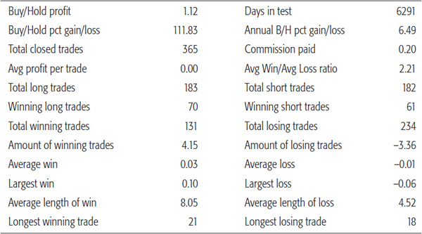
On the face of it, the number of losing signals of 234 to 131 winners looks pretty grim. However, when you look at the more detailed report of Table 34.3, the average win was 2.2 times greater than the average loss, which shows this system did a reasonable job of cutting losses short.
TABLE 34.3 Treasury Bonds Using the 28/2/-2 Combination, 1981–1998
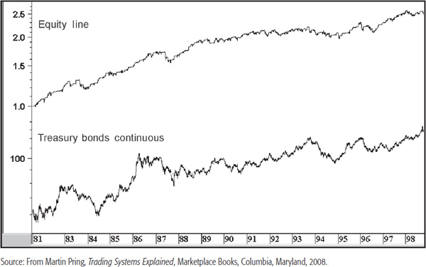
The top panel of Chart 34.4 shows the equity line. The starting amount of $1 was increased to $2.55. Even though the system trailed the buy-hold approach, there were no major drawdowns in terms of peak-to-trough equity. The one in 1994 of 10 percent was the worst. Not bad, considering the 150 percent gain was achieved at a 9.4 percent annualized rate.
CHART 34.4 Treasury Bonds, 1981–1998, Featuring the 28/2/–2 Price Oscillator System
Other tests on many closed-end mutual funds covering the 1980s and 1990s have shown that the 28/5/–5 combination of a 28-day MA and a close divided by a 28-day MA using +5 and –5 as the overbought/oversold triggering points worked consistently well.
One important principle that should be followed when designing a system incorporating several triggering mechanisms is to make sure it incorporates different indicators based on different time frames. The contrasted time frames are important because prices at any one time are determined by the interaction of many different time cycles. We cannot make provisions for all of them, of course. If we can ensure there is a good time difference that separates the indicators used in the construction, we will at least have made an attempt to monitor more than one cycle.
A system I devised in the late 1970s combines an MA crossover with a signal from two rate-of-change (ROC) indicators. These are a 10-week simple MA, a 6-week ROC, and a 13-week ROC. Thus, we have two different types of indicators: a trend-following MA and two oscillator types. The system also consists of three different time frames. The buy and sell rules are very simple. Buy when the price is above the 10-week MA and both ROCs are above zero. Sell when all three go negative, that is, when the ROCs cross below zero and the price crosses its MA. Signals cannot be generated unless all three agree. This is because we want to make sure the various cycles reflected in the three different time frames are all in gear. Originally, when I introduced this system, it was applied to the pound/dollar relationship because it was one that trended very consistently.
Let’s take a close look at Chart 34.5 to see how it works by starting off with a simple 10-week MA crossover between mid-1974 and 1976. Buy signals are once again indicated by the upward-pointing arrows and short positions by the downward-pointing ones. There were 13 signals for a total profit of $0.19 on an initial $1 investment, from both the long and the short side. This compares to the buy-hold approach, with a loss of almost $0.70. Taken on its own, this was a fairly commendable performance, but let’s remember that for a significant portion of the time, that is, most of 1975 and 1976, the British pound was in a sustained downtrend. It is true there were a number of whipsaws in late 1975 and early 1976. These are shown in the two ellipses, but they were of minor consequence as it turned out.
CHART 34.5 British Pound System and a 10-Week MA

The next step is to introduce a 13-week ROC. Buy and sell signals are triggered when the 13-week ROC crosses above and below its zero reference line. This approach, shown in Chart 34.6, nets a gain of $0.23 with six signals. This was better than the results with the MA crossover, especially since fewer signals dramatically reduced the potential for whipsaws. Even so, there were a couple of nasty whipsaws in 1976.
CHART 34.6 British Pound System and a 13-Week ROC
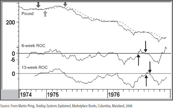
The next step is to introduce a second ROC indicator to filter out some of the whipsaws. A 6-week ROC was chosen mainly because it spans approximately half the time span of the 13-week series. The result was an improved $0.24, but the number of signals increased to 12. The 6-week ROC is shown in the middle panel of Chart 34.7.
I put all three indicators together in Chart 34.7 so you can see how their integration improves things. The actual result was a slight increase in profit over the previous 6-week ROC test. However, the important thing was that the signals were reduced to only three. A closer look at Chart 34.7 shows that the first sell comes in October 1974, as the 6-week ROC follows the others into negative territory. Then, in December, the 13-week ROC crosses above zero, and this is closely followed by an MA crossover. Finally, the 6-week series moves above zero for a buy signal. All three then move into negative territory in April 1975. The MA and 6-week ROC go bearish simultaneously, and this is then followed by the 13-week series. The system stays bearish all the way through late 1976. It almost goes bullish when the price crosses its average and the 6-week ROC goes positive in February 1976. However, the 13-week series, which had been bearish, now goes bullish, but by this time, the currency had slipped below its MA and the 6-week series fell below zero. As a result, all three indicators were never in agreement. The same is true in the July–August period of 1976 when the two ROC indicators take turns in being bullish and bearish. This was a type of a negative complex divergence described in Chapter 13. The combination of all three indicators works extremely well in this environment.
CHART 34.7 British Pound System and Three Indicators
This is about as good as it gets.
I originally introduced this approach in my book International Investing Made Easy (McGraw-Hill, 1981) with some hesitancy because there was obviously no guarantee it would continue to operate profitably. It was subsequently reintroduced in the third edition of this book in 1992 with the same proviso. What I said was, “It is important to understand this approach will not necessarily offer such large rewards in the future. The example of the British pound must be treated as the exception rather than the rule, but it is introduced to give you an incentive to experiment along these lines.”
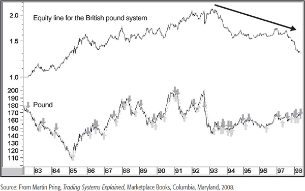
The system continued to work extremely well, as you can see by looking back at the equity line in the upper panel in Chart 34.8. However, I am glad I used the cautionary statement, because once we move past 1993, the system fell apart. Just look at the declining equity line between 1993 and 2002 in Chart 34.8. Indeed, though it made money for the next 10 years, the peak 1993 equity has never been surpassed. The initial drop was due to the many whipsaws arising from the trading range that followed the drop from $2.00 in 1993. This goes to show that even if a system works well for 20 years, as this one had, market conditions can and do change, so you must be prepared for such instances. Obviously, we do not know until sometime after the fact that the market environment was different. Is there anything we can do to avoid such situations? One possibility is to run a very long-term MA or trendline through the equity line.
CHART 34.8 British Pound System Results, 1983–1998
In Chart 34.9, I have plotted a 300-week simple MA against the equity line of the three-indicator pound system when applied to the Hang Seng Index. I used 300 weeks because I felt it necessary for the system to undergo a fairly long period before it can be considered out of touch. The idea is when the equity line crosses below the MA something is seriously wrong with the system, and it should be at least temporarily abandoned. At this point, it would make sense to reappraise it and see if it could be improved, and I do not mean by introducing special rules to block out a bad period. You could also wait until the equity line crosses back above the MA again, but in the case of the “busted” pound system, as far as the pound was concerned, even that approach was problematic. Unfortunately, such eventualities are unavoidable, which is why it’s a good idea to diversify among securities and systems in order to reduce risk.
CHART 34.9 British Pound System Applied to the Hang Seng Index, 1981–2012

So far, we have just considered particular securities or markets in isolation, using statistically derived data from that security alone. An alternative approach is to adopt a tried and tested intermarket relationship as a cross-reference.
Better results are often obtained in this way. An intermarket relationship develops when one market consistently influences another. The first step is to rationalize why such a relationship exists in the first place. Perhaps the most basic one is between equities and short-term interest rates. This was described in Chapter 31, where it was established that changes in the trend of short-term interest rates lead equity prices.
What we do not know is the lead time or the magnitude of the ensuing stock rally. The answer is to classify the trend of money-market prices, which is what the inverted short rate actually is, with an MA crossover. When a rising trend of money-market prices has been established, it is then time to look at the trend of equities to see when they respond. The rationale is that a rising trend of money-market prices sets the scene for an equity bull market. However, this is not confirmed until the S&P Composite crosses above its MA. Just think of this as something akin to an unconscious swimmer receiving mouth-to-mouth resuscitation. You know the treatment is good for the patient, just as falling rates are good for equity prices. However, we do not know how much treatment is required and whether the patient will recover until he or she is able to breathe by him-or herself. In our analogy, the stock market is shown to respond to the interest-rate treatment when it crosses its MA.
Here is how it works. Look at Chart 34.10. In October 1981, the inverted commercial paper yield crosses above its 12-month MA (shown in the ellipse), indicating the environment is now bullish for equities. However, the equity market does not respond by bottoming out until August 1982. When the S&P rallies above its 12-month MA (A), it indicates that the market is responding to the positive interest rate environment. In this case, the crossover comes in August 1982. At that time, both trends are bullish and so is the system. It remains positive until either series moves back below its average, which, in this case, developed in June 1983 (B). It then goes bullish again in January 1985 (C).
CHART 34.10 S&P Composite, 1980–1988, versus 3-month Commercial Paper Yield
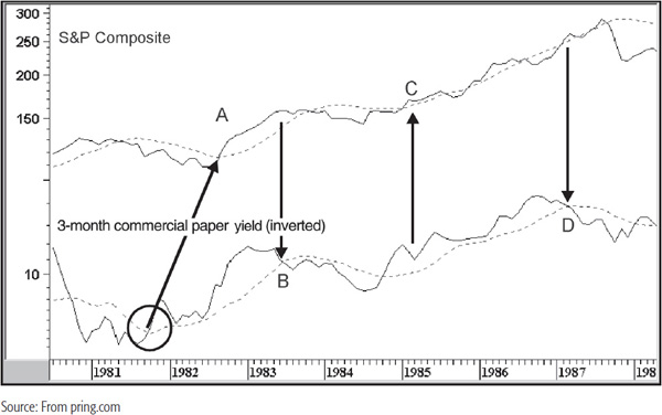
Finally, the inverted yield falls below its average in early 1987 (D). The market continues to rally, but the system is no longer bullish. In most instances, it would be better to generate the sell signals after the S&P crosses below its average. In this instance, though, the 1987 crash was over before the average was penetrated. Since the risk increases as the money-market series crosses below its average, it is probably best to act on the signal in two parts. This would involve taking off half the position as the money-market series goes negative and then liquidating the rest when the S&P crosses its average.
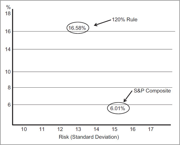
Figure 34.5 compares the risk and reward for the system between 1900 and 2009 to that for the S&P Composite. The vertical axis measures the monthly reward on an annualized basis, and the risk is measured on the horizontal axis. In this sense, risk is measured as volatility. The best place for any system to be is in the top-left corner, often referred to as the northwest quadrant. This is where the reward is high and the risk, or volatility, is low. In the case of this system, you can see that the risk was slightly lower than that for the S&P, but the reward was substantially higher. At Pring Turner Capital, we call this the 120 percent rule because it has had such an excellent and consistent track record for over 100 years.
FIGURE 34.5 The 120% Rule Risk versus Return
The system says nothing about periods when the market is above its average and rates are not, since those are obviously bullish periods as well. However, once rates move above their 12-month MA, there is a real danger that the next correction could be the first downleg in a bear market. It is true that sooner or later the S&P Composite will cross below its MA, thereby stopping us out, but why run the risk when good returns and little volatility can be had under more favorable conditions? During those periods when both were in a negative mode, the annualized loss was 9.58 percent.
If you are a short-term trader, you probably feel this approach is worse than useless. However, it can be put to very good use if you realize that when the system is bullish, short sell signals are more likely to result in losses. They are not just going against the main trend, but are occurring in one of the most positive equity environments you can get. By the same token, this knowledge can be used to take positions yourself on the long side when a short-term buy signal is triggered. I am not going to say that sharp corrections will never happen when this system is positive, because there have been periods such as 1971 when a fairly large retracement move did materialize. It is merely that when the system is positive, the odds favor strong short-term rallies and whipsaw reactions.
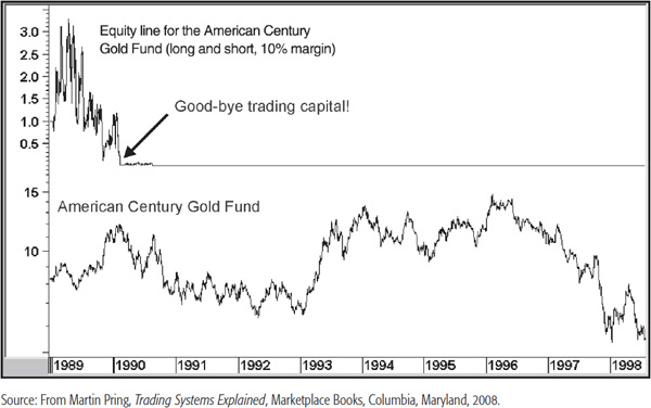
All the systems described here were tested on a cash basis with no margin. You might think that it makes sense to go out and apply a system using lots of margin. That way the gains would multiply. In actual fact, this is not necessarily the case. Chart 34.11 shows a simple 10-day MA crossover system using no margin, and Chart 34.12 shows it using a 10 percent margin requirement. Since the initial trades were losers, the account was wiped out in just over a year. Remember: Leverage works both ways.
CHART 34.11 American Century Gold Fund, 1989–1998
CHART 34.12 American Century Gold Fund, 1989–1998
1. There are two ways in which systems can be used: act on each signal without question, or use the signals as a filter so the current system becomes one more indicator in the weight-of-the-evidence approach.
2. The principal advantage of a mechanical system is that it removes subjectivity and encourages the adoption of discipline.
3. No system will ever work all of the time. It is important to understand the pitfalls of automated systems so that they can be programmed out.
4. Systems should be designed to take account of the fact that there are two different types of market environment: trading range and trending.
5. Because no system works perfectly, it should be exhaustively tested before being applied to the marketplace.
6. The use of any system should involve diversification to spread the risk for any period where it does not operate successfully for a specific security.
7. Incorporating a tried and tested intermarket relationship into the system acts as a cross reference and usually enhances results.
8. The use of margin exaggerates the results, both on the upside and the downside. The actual performance will depend on the chronological sequence of the good and bad signals.