All the effects of nature are only mathematical results of a small number of immutable laws.
P. S. LAPLACE
In the seventeenth century one of the most pressing problems of the times was time itself. The increasing scientific activity, particularly in an age which had decided to measure and to seek quantitative laws, created the need for convenient, accurate methods of measuring time. Moreover, as we have already had occasion to mention in other connections, the seventeenth and eighteenth centuries were concerned with the very practical problem of improving the method by which ships determined their longitude at sea. Here a good clock is the simplest answer. Suppose that the longitude of a given place on land is known and that a ship has on board a clock set to agree with the time prevailing at that given locality. Since the earth turns through 360° of longitude in one day, it turns through 15° in each hour. Hence for each 15° that a ship is west, say, of the fixed locale, midday occurs one hour later compared to the time at the fixed position on land. If a ship’s officer notes (by means of the sun’s position) when midday occurs at his position at sea and finds, for example, that his clock reads 3 o’clock whereas it should, of course, read 12 o’clock, he knows that the longitude of his position is 45° west of the given reference locality on land. We can see then why scientists decided to search for a reliable and accurate clock.
The thought which suggested itself almost at once was to look for some physical phenomenon which repeated itself regularly. The day contains 24 hours; hence when the number of repetitions per day is known, the duration of each repetition is readily calculated. Where then could one find a repetitive or periodic physical phenomenon? Two prospects attracted the attention of seventeenth-century scientists. The first of these was the motion of a mass, called a bob, attached to a spring and oscillating up and down, and the second was the motion of a pendulum, that is, a bob attached to a string and swinging to and fro. Now first reactions to the possibility of using the motion of a bob on a spring or a pendulum as a measure of time are apt to be negative. The bob on a spring, for example, does go through each cycle, that is, each complete up and down motion, in the same time so far as the eye can judge, but the motion soon dies down. The same is true for the pendulum. But, if air resistance could be minimized or perhaps compensated for, then these motions might become truly periodic and should therefore merit investigation. The scientist or mathematician who expects to see at once the solution of a problem he sets out to study will never accomplish much. The best he can hope for at the outset is an idea or a clue to pursue.
In this chapter we shall examine first the physical problem of the motion of a bob on a spring, a prime example of oscillatory motion. To study such motions mathematicians created a new class of functions, the trigonometric functions. We shall then discuss these functions and see how they are used to derive some knowledge about the physical problem which motivated their introduction. Surprisingly, trigonometric functions proved to be admirably suited for the study of sound, electricity, radio, and a host of other oscillatory phenomena. Of these latter developments we shall learn more in the next chapter.
The problem of investigating the motion of a bob on a spring was undertaken by one of the greatest experimentalists in the history of physics, the Englishman Robert Hooke (1635–1703). Hooke was professor of mathematics and mechanics at Gresham College. His claim to fame also rests upon his success as an inventor. To his credit are a telescope moved by a clock mechanism and devices for measuring the moisture in the atmosphere, the force of the wind, and the amount of rainfall. He improved the microscope, the barometer, the air pump, and the telescope. One of his findings, namely, that white light passed through thin sheets of mica breaks into many colors, parallels Newton’s work on light. He also discovered the cell structure of plants. Hooke was very much interested in designing a useful clock and thought that springs would furnish the essential device. While working on the action of springs, he discovered a basic law, still known as Hooke’s law, which we shall discuss later.
Let us follow Hooke in studying the motion of a bob on a spring. The upper end of the spring is attached to a fixed support, and a bob is attached to the lower end. Because gravity pulls the bob downward, the spring will be extended until the tension in the spring offsets the force of gravity. The bob then comes to rest in some position which is called the rest or equilibrium position (Fig. 18–1). If one now pulls the bob downward some definite distance below the rest position and then releases it, the bob moves up to the rest position, continues past that point to some highest position, and then moves downward. When it reaches the point to which it had been pulled down, it starts upward and repeats its former motion. Following Galileo’s plan of idealizing the physical situation, let us suppose that air resistance is negligible. (Strictly speaking, energy is also lost in the expansion and contraction of the spring, but this loss is negligible.) Then the bob will continue to move up and down endlessly.
Fig. 18–1.
A bob on a spring.
To begin to get some mathematical description of this motion let us introduce a Y-axis alongside the bob (Fig. 18–1) and suppose that y = 0 corresponds to the rest position of the bob. When the bob is above or below the rest position, the bob is said to be displaced and the distance that it is above or below the rest position is called its displacement. To distinguish displacements above from those below the rest position, we shall call the former positive and the latter negative. Each displacement may then be described by a value of y. Thus ![]() means that the bob is
means that the bob is ![]() unit below the rest position.
unit below the rest position.
To study the motion of the bob mathematically, it would be most helpful if we could find the formula which relates the displacement of the bob and the time it is in motion. Let us therefore seek such a formula.
No one of the formulas that we have considered thus far would be useful to represent the motion of the bob, for the peculiarity of the present phenomenon is that after each up and down motion, or oscillation, has been completed, the displacements go through their former sequence of values. Hence we apparently must seek a new type of formula which expresses the periodic character of the motion of the bob. We do not seem to have any clue, but a little imagination may supply one.
Suppose a point P moves around a circle of unit radius at a constant speed. Let us denote some of its positions by P1, P2, . . . (Fig. 18–2). We can, if we wish to, introduce a point Q on the vertical line through the center O such that Q always has the same height that P has above or below the horizontal through O. The point Q is called the projection of P on the vertical line. Thus to the position P1 of P there corresponds Q1; to P2 there corresponds Q2; and so on. Why should we introduce the point Q? Well, let us imagine P moving around the circle through many revolutions starting from the position S at the right. What does its “shadow” Q do? It moves up from O to a highest position, moves down again to O, moves past O to a lowest position on the vertical line, moves up again to O, and then repeats this up and down motion. The motion of Q certainly seems to have the essential characteristics of the motion of the bob on the spring. Hence perhaps by pursuing further the motion of Q we may obtain the function we are seeking.
Fig. 18–2.
Successive positions of a point P which moves around a circle at a constant velocity, and the corresponding positions of Q.
Fig. 18–3
Fig. 18–4
Let us introduce coordinate axes as shown in Fig. 18–3. If P starts from the X-axis and reaches, say the position P1, then we may describe the position of P by the angle A shown in the figure. The height of Q above the X-axis is the same as the y-value of P. Now
![]()
Hence
Thus if the position of P is described by the angle A, then the position of the corresponding point Q on the vertical line is given by (1).
But now suppose P has moved to the position P4 shown in Fig. 18–4. The angle A which describes the position of P4 is the obtuse angle shown in the figure. This angle is no longer an acute angle of a right triangle, and we therefore have no right to speak of sin A. However, let us extend the meaning of sine so that, by definition, sin A is the y-value of P4. Since the height of Q4 above Q equals the y-value of P4, we may continue to write y = sin A to describe the position of Q. That is, the distance of Q from O on the vertical line will be given by y = sin A.
Fig. 18–5
Fig. 18–6
Fig. 18–7
Suppose next that P occupies the position P5 shown in Fig. 18–5. The angle A which describes how far around the circle P has moved is now the angle shown. Let us agree again that by sin A we shall mean the y-value of P5, which is also the distance below the X-axis of the point Q5. Then we again may write y = sin A to describe the position of Q. Note that y is now a negative quantity.
If P reaches the position P6 shown in Fig. 18–6, then its position is represented by the angle A shown, and if we again agree to mean by sin A the y-value of P6, we shall be able to say here too that y = sin A describes the position of Q. In this instance also, y is a negative quantity.
As P returns to the X-axis and starts to repeat its revolution, the angle A which describes the position of P will now be 360° plus some additional angle (Fig. 18–7). It is only by including 360° for each revolution of P that we can keep track of the number of revolutions. However, let us note that the y-values of P will recur in precisely the same order in which they appeared on the first revolution. Despite the fact that on the second revolution the values of A are larger than 360°, we shall continue to mean by sin A the y-value of P. Thus sin 390° will be the same as sin 30°. As P goes through its second revolution, Q repeats the motions of the first revolution. Hence it will still be true that y = sin A describes the position of Q on the vertical line. With each revolution of P, the y-values repeat, although the angle A increases by 360°. Since the motion of Q also repeats, its position on the vertical line will continue to be represented by y = sin A.
Fig. 18–8.
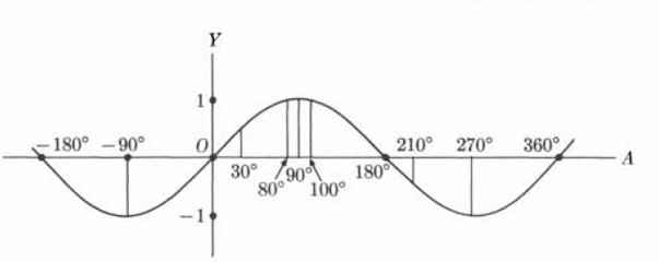
The graph of y = sin A.
If P were to revolve in the clockwise direction, then we would make only-one change, i.e., call the values of A negative. The y-value of P, wherever it is, is still, by definition, sin A and this y-value would represent the position of Q.
Let us survey what we have done. To describe mathematically the position of the point Q, we have introduced a new function: y = sin A. When A is an acute angle, as in Fig. 18–3, then sin A has the old meaning; that is, it is the ratio of the side opposite angle A to the hypotenuse of the right triangle in which A lies. (In the present case the hypotenuse is 1.) But when A is larger than 90°, then the equation y = sin A is a definition of what we mean by sin A. Since there is a definite y-value for each value of A, positive or negative, we do indeed have a function.
To appreciate the nature of this function let us graph it. Figure 18–8 shows the graph. The values of A are plotted along the horizontal axis, and the corresponding y-values are plotted in the usual way.
Do we know the precise numerical value of y for each value of A? We do. For values of A which are between 0° and 90°, the y-values are the ordinary sine values which we find in our trigonometric table. In the interval from 90° to 180°, the values of sin A repeat, but in reverse order, the values which sin A has when A varies from 0° to 90°. This statement implies that sin 100° = sin 80°, sin 110° = sin 70°, and so forth. Stated in more general terms:
In the interval from 180° to 360°, sin A has the same numerical values as when A varies from 0° to 180°. However, now sin A is negative. Thus sin 210° = −sin 30°; sin 220° = −sin 40°; and in general:
Since for each 360°-interval beyond the interval 0° to 360° sin A repeats the values that it has in the interval from 0° to 360°, sin 390° = sin 30°; sin 400° = sin 40°; and so on. In symbolic form,
The values of sin A for negative values of A are also shown in Fig. 18–8. If we look at the figure, we see that for any negative A-value, sin A is the negative of the sine of the corresponding positive A-value, That is, sin (−30°) = −sin (30°); sin (−50°) = −sin (50°), and in general:
Thus we have arrived at a definition of the function y = sin A for all values of A. Since we know quantitatively what sin A is for values of A between 0° and 90°, formulas (2) through (5) enable us to calculate sin A for all other values of A. The function we have just introduced is called a periodic function because the y-values repeat themselves in every 360°-interval of A-values. The interval of 360° is called the period of y = sin A, and the entire set of y-values in one period is called the cycle of y-values.
1. Using formulas (2) through (5) or Fig. 18–8, express the following sine values as sines of angles between 0° and 90°.
a) sin 120°
b) sin 150°
c) sin 210°
d) sin 260°
e) sin 270°
f) sin 300°
g) sin 350°
h) sin 370°
i) sin –50°
j) sin 750°
2. What is the largest value of sin A? What is the smallest value of sin A?
3. At what value of A between 0° and 360° does the function y = sin A reach a maximum?
4. Why is y = sin A called a periodic function?
5. What purpose does the function y = sin A serve with respect to the location of Q, the projection of P?
6. What is the relationship between the function y = sin A and the trigonometric ratio sin A studied in Chapter 7?
7. Describe how sin A varies as A varies from 0° to 360°; from 360° to 720°.
8. For how many values of A between 0° and 360° is sin A = 0.5?
9. Distinguish between the period and the cycle of y = sin A.
Thus far we have described the size of angles in degrees. There is, however, no need to stick to this unit. Let us return to the motion of the point P in Figs. 18–3 through 18–7. The size of angle A can be specified by describing the arc length traversed by P from its starting point on the X-axis. This arc length is as much a measure of the size of angle A as the rather arbitrary agreement that a complete revolution of one side of A should be 360°.
Suppose that we agree to use the arc length traversed by P as a measure of A. How do we express in this new unit an angle of 90°, for example? When A is 90°, P has traversed one-quarter of the entire circumference. But the entire circumference of a circle of unit radius is 2π. Then the size of A in the new unit is π/2, that is about 1.57. We call this new unit radians. Thus an angle of 90° is also one of π/2 or 1.57 radians.
The advantage of radians over degrees is simply that it is a more convenient unit. Since an angle of 90° is of the same size as an angle of 1.57 radians, we now have to deal only with 1.57 instead of 90 units. The point involved here is no different from measuring a mile in yards instead of inches. If yards are just as good on other grounds, then it is far more convenient to speak of 1760 yards than 63,360 inches.
Fig. 18–9.
The graph of y = sin A when A is measured in radians.
The fact that we measure angles in radians does not disturb at all the meaning of the function y = sin A. Instead of stating that sin 90° = 1, we simply say that sin (π/2) = 1. The same applies to any other value of A in the sinusoidal function we have introduced. Suppose, for example, that we wished to find the value of y = sin A when A = π/6. Because our table is set up in degrees, we note first that an angle of π/6 is of the same size as 30°, for π/2 radians is the same as 90°. Now from our tables we see that sin 30° = 0.5, and so sin (π/6) = 0.5.
Since we shall be using radians a good deal, we may as well become familiar with the function y = sin A when A is expressed in radians. Figure 18–9 shows the same function as Fig. 18–8 except that the units of A are now radians.
1. Express the sizes of the following angles in radians: 90°, 30°, 180°, 270°, 360°, 420°.
2. The sizes of the following angles are in radians. Express the same angles in degrees.
π/2 2π/3 5π/2 3π −π/2 1
3. Find the value of
a) sin π
b) sin (π/2)
c) sin (π/3)
d) sin (3π/2)
e) sin 3π
f) sin (5π/2).
4. Describe how sin A varies as A varies from 0 to 2π, as A varies from 2π to 4π.
The function y = sin A has a maximum value of +1 and a minimum value of −1. The maximum y-value, incidentally, is called the amplitude of the function. Such a function, even if it were suitable in all other respects, could not represent the motion of a bob whose maximum displacement is 2 or 3, say. This difficulty is easily obviated. Now that we have y = sin A, we can readily manufacture hundreds of new functions whose amplitudes are whatever we choose to make them. Consider, for example, y = 2 sin A. How does this function behave compared to y = sin A? The answer is immediate. For any value of A, y = 2 sin A is twice as much as y = sin A. Thus when A = π/4 or 45°, sin A = 0.71, and 2 sin A is 1.42. Figure 18–10 shows how y = 2 sin A looks compared to y = sin A. If we want a sine function with amplitudes 3, ![]() , or any other number, we can write one down immediately. As is evident from the nature of the function y = 2 sin A, the function
, or any other number, we can write one down immediately. As is evident from the nature of the function y = 2 sin A, the function
y = D sin A
has amplitude D.
Before we can use functions such as y = sin A or y = 3 sin A to represent the motion of a bob on a spring, we must clear one more hurdle. The function we seek should represent a relationship between displacement and time. The y-values of our functions do indeed represent the displacement of a point Q which moves up and down on a line, but our independent variable is an angle. Suppose, however, that the point P revolves around the circle ƒ times in one second. Then, since for each revolution the angle A increases by 2π radians, the size of the angle which describes the amount of revolution of P in one second is 2πf. If the point P revolves for t seconds and makes ƒ revolutions per second, it will make ft revolutions in t seconds. The angle generated during these ft revolutions will be 2πft. Hence, the value of A in t seconds will be 2πft. Thus the function y = sin A becomes
Fig. 18–10. Comparison of y = sin A and y = 2 sin A.
Fig. 18–11. The graph of y = sin 2πt.
This function requires some study. Suppose the point P makes one revolution per second. Then f = l. The function (6) then is y = sin 2πt. As t increases from 0 to 1, the quantity 2πt will increase from 0 to 2π. We must now ask, How will sin 2πt vary as 2πt varies from 0 to 2π? Since the angle which 2πt describes now varies from 0 to 2π, the function will go through the entire cycle of sine values. However, if we now label our horizontal axis with time values, we obtain the graph shown in Fig. 18–11.
Next let us consider a slightly more difficult case. Suppose the point P makes 2 revolutions per second so that f = 2. As t increases from 0 to ![]() , 2π · 2t will increase from 0 to 2π and sin 2π · 2t will go through the entire cycle of sine values. As t increases from
, 2π · 2t will increase from 0 to 2π and sin 2π · 2t will go through the entire cycle of sine values. As t increases from ![]() to 1, 2π · 2t increases from 2π to 4π. Then sin 2π · 2t takes on the values corresponding to angles from 2π to 4π. But in this range the sine function takes on the same values as it does in the range from 0 to 2π. Hence in the entire interval 0 to 1 for t, the graph will be as shown in Fig. 18–12. The conclusion, which emerges clearly from the graph, is that
to 1, 2π · 2t increases from 2π to 4π. Then sin 2π · 2t takes on the values corresponding to angles from 2π to 4π. But in this range the sine function takes on the same values as it does in the range from 0 to 2π. Hence in the entire interval 0 to 1 for t, the graph will be as shown in Fig. 18–12. The conclusion, which emerges clearly from the graph, is that
y = sin 2π · 2t
goes through 2 complete cycles in one second or, as one says, it has a frequency of 2 cycles per second.
Fig. 18–12. The graph of y = sin 2π · 2t.
We can now anticipate what happens for any ƒ. The function
y = sin 2πft
will go through ƒ cycles in one second, or it has a frequency of ƒ cycles per second.
To increase the amplitude of any of these functions, we have but to introduce the factor D. Thus the function
will have a frequency of ƒ cycles per second and an amplitude of D. Let us note that while ƒ is the number of revolutions per second of P, it is also the number of oscillations per second of Q.
The y-values of formula (7) oscillate above and below the zero value as t varies. We can make the number of oscillations per second what we please by merely inserting the proper value of ƒ and we can do the same with respect to the amplitude by inserting the proper value of D. Of course, we do not know the proper values of ƒ and D which fit the motion of a bob, but we shall see in the next section that it is not difficult to determine them.
Let us summarize what we have accomplished. We sought to represent the motion of a point which oscillates back and forth on a straight line. We were able to do so by introducing a point Q which is the projection of a point P moving around a circle at a constant velocity. Because the y-value of P equals the displacement of the oscillating point Q and because the y-value of P is expressible as a sinusoidal function, we can represent the motion of the oscillating point Q by such a function. That the approach to the oscillating point Q through the circle should be successful may be surprising, but, as Aristotle pointed out, “There is nothing strange in the circle being the origin of any and every marvel.”
1. Find the value of 2 sin A when A is 30°, 90°, π/2, π/3.
2. What is the maximum value of 3 sin A? the minimum value?
3. What is the amplitude of y = 4 sin A?
a) sin 2t when t = π/4, π/2, 3π/4, π;
b) sin 3t when t = π/6, π/3, π/2, 2π/3.
5. What is the shape of the graph of y = sin 2π · 2t as t varies from 1 to 2?
6. Graph the function y = sin 2π · 3t as £ varies from 0 to 1.
7. Graph the function y = 2 sin 2π · 2t as t varies from 0 to 1.
8. What is the frequency (in one second) of y = sin 2π · 10t?
9. Find the value of
a) y = sin 2π · 2t when t = ![]() ,
, ![]() ,
, ![]() ;
;
b) y = sin 2π · 4t when t = ![]() ,
, ![]() , 1;
, 1;
c) y = 2 sin 2π · 3t when t = ![]() ,
, ![]() ,
, ![]() .
.
What we have seen in the preceding article is that if a point P moves around a circle of unit radius at a constant speed and makes ƒ revolutions per second, then the projection Q of P onto the vertical diameter moves up and down this diameter, and the displacement y of Q from its central position at O can be represented by formula (6), namely,
Moreover, if we wished to represent the same kind of oscillatory motion but with an amplitude D instead of 1, we have merely to modify (8) to read
Our goal, however, is to represent the motion of the bob on the spring. Before we can do this we must learn one more fact about the motion of Q, namely, the acceleration of Q. The motion of Q, as we approached it, was determined by the motion of P which travels around the unit circle at a constant speed, say v. If an object moves along a circular path, then we know from our work in Chapter 15 that it must be subject to a centripetal acceleration, and by formula (24) of Chapter 15 this centripetal acceleration is v2/r, where r is the radius of the circle. In our case, since P moves on a circle of unit radius, r = 1, and so the centripetal acceleration of P is v2. This acceleration is directed toward the center of the circle.
We are, however, interested not in the motion of P, but in the motion of Q, which moves in the same way as the vertical motion of P. Hence we should seek the vertical acceleration of P. We learned in Chapter 14 that even though an object moves along a curve, we can study its motion by considering the horizontal motion and the vertical motion separately. By Galileo’s principle these two motions are independent of each other. What we should like then is the vertical acceleration of P. When we considered the motion of a shell shot from a cannon inclined at an angle A to the ground, we found the horizontal and vertical velocities by dropping perpendiculars from the end point of the line segment representing velocity onto the horizontal and vertical axes (Section 14–4).
Fig. 18–13.
Determination of the vertical acceleration of P.
Now acceleration, like velocity, is a directed quantity or a vector. Moreover, the acceleration determines the velocity. Hence we should compute the vertical acceleration of the point P in the same manner as we computed the vertical component of the velocity of the shell. Figure 18–13 shows the centripetal acceleration v2 of P as a line segment directed toward the center of the circle. If we drop a perpendicular from the end point of this line segment onto the vertical line through P, we obtain the vertical component of the acceleration. Angle A in the figure determines the position of P. We see, then, that the vertical component of the acceleration, which we shall denote by a, is
a = v2 sin A.
We know, however, from (1) that
sin A = y,
where y is the ordinate of P. Hence
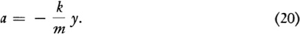
a = v2y.
However, since the acceleration is directed downward when y is positive, we must write
If now the moving point P makes ƒ revolutions per second, then P covers ƒ circumferences per second; that is, v = 2πf and v2 = 4π2f2. We substitute this result in (10) and obtain
as the acceleration of the vertical motion of P or of its shadow Q on the Y-axis.
What we have shown then is that the motion of Q, which is described by the formula
is subject to an acceleration of
We may now undertake to represent mathematically the motion of the bob on the spring. We know that this motion is periodic and has a definite frequency and amplitude. However, we do not know that the motion is really sinusoidal; that is, as t varies, do the displacements of the bob follow precisely the variation of y in a function of the form
If, for example, the motion of the bob should be faster on the upper half of its path than on the lower half, it could still have the same period for each complete oscillation and perform a fixed number of oscillations per second. Yet the motion would not be of the form (14). We need a little more insight into the motion of the bob than we now have.
This insight into the action of bobs on springs was supplied by Robert Hooke. The principle he discovered, still known as Hooke’s law, is very simple. We all know that if we stretch or compress a spring, the spring seeks to restore itself to its normal length; that is, when stretched or compressed the spring exerts a force. Hooke’s law says that the force is a constant times the amount of compression or extension. In symbols, if L is the increase or decrease in length of the spring and F is the force exerted by the spring, then F = kL, where k is a constant for a given spring. The quantity k is called the spring or stiffness constant and it represents the stiffness of the spring. If k is large, the spring exerts considerable force even for small L.
We shall now see what we can deduce from Hooke’s law. Suppose that a bob of mass m is attached to a spring. Then we know that gravity pulls the bob downward some distance d where the bob comes to rest (Fig. 18–14). The rest position is reached when the force of gravity acting on the bob, or the weight of the bob, just offsets the upward force exerted by the spring. Now the force of gravity is 32m, and, according to Hooke’s law, the upward force exerted by a spring which is pulled downward a distance d is kd. Since at the rest position these two forces just offset each other, we have
Fig. 18–14.
A bob on a spring in the rest position (center) and pulled down a distance y (right).
Now suppose the spring is pulled downward an additional distance y. If we use the convention agreed upon in Section 18–2 that displacements above the rest position are to be positive and below the rest position negative, then the total extension of the spring is now d − y because y itself is negative. The force that the spring exerts in an upward direction is, by Hooke’s law,
However, the weight of the bob, or 32m, exerts a constant downward force. Hence the net upward force is kd − ky − 32m. In view of equation (15) the net upward force is −ky. We now apply Newton’s second law of motion, which says that when a force is applied to a mass, the force equals the mass times its acceleration. Thus we have
or, by dividing both sides of this equation by m,
Formula (18) is the basic law governing the motion of the bob on the spring. For, suppose the bob is pulled down some distance and then released. The spring exerts a force which pulls the bob back toward its rest position. The acceleration created by this force is precisely that given by (18). The acceleration now determines the velocity of the bob and the velocity determines the distance covered by the bob in any specified interval of time. The argument we are presenting here is in principle the same as the one we used in Chapter 13, where we discussed the motion of a body which is raised some distance from the surface of the earth and then dropped. In this situation, gravity immediately exerts an acceleration of 32 ft/sec2, and thereafter the velocity and distance fallen by the object are determined. Of course, in the present case the acceleration is a more complicated expression, and the subsequent motion is not simply in one direction, but the argument is of the same nature.
We should now compare formula (13), namely,
and formula (18),
In both cases the acceleration is a constant times the displacement. The constant is 4π2f2 in the former case and k/m in the latter. When the acceleration is given by (19), the motion itself [see (12) and (13)] is represented by
Since the acceleration (20) is precisely of the same form as (19), except for the label of the constant, and since the acceleration determines the motion, the motion of the bob must also be representable by a formula of the form (21).
However we do not know what f is in the case of the bob. But k/m in the case of the bob plays the role of 4π2f2 in the case of the motion of the point Q. That is
![]()
so that

and

or
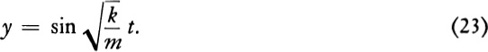
In other words, if we let f in (21) be the value given by (22), we can write the formula for the bob’s motion in terms of the quantities k and m. Thus if we substitute this value of f in (21), we obtain

or
We made one misleading statement in the preceding discussion. We said that the acceleration of the bob determines the motion of the bob, and so the formula of the bob’s motion must be of the form (21). The acceleration does determine the essential characteristics of the motion, but the initial velocity and initial displacement do have some effect. This point may become clearer if we compare the present case with the vertical motion of objects. All bodies rising or falling near the surface of the earth are subject to an acceleration of 32 ft/sec2, and this fact determines the essential nature of the motion. But if a body is thrown up into the air, the final formula depends also on the initial velocity given to the object and on the position from which it is thrown up. In the case of the bob, if it is pulled down to a distance D below the rest position and then released, this initial position must enter into the formula for the motion. To complete our determination of the formula we are obliged, with the limited mathematics at our disposal, to call upon observation, which tells us that in each oscillation the bob will rise to a height of D above the rest position and then descend a distance D below it. That is, the amplitude of the motion, D, is determined by the initial displacement. Thus the final formula for the motion of the bob is
We can now draw several conclusions about the motion of the bob. Formula (22) gives the frequency of the bob’s motion in terms of k and m. We see that the spring constant k, which represents the stiffness of the spring, and the mass m of the bob determine the frequency of the motion. If we wished to have the bob make, for example, two complete oscillations per second, we could pick values of k and m so that f in (22) should be 2. The period of the bob’s motion, that is, the time required to make one oscillation, is

or
As Hooke observed, this formula for the period is immensely significant. The period is independent of the amplitude of the motion; that is, whether one pulls the bob down a great distance or a short distance and then releases it, the time for the bob to go through each complete oscillation will be the same.
This fact is immensely useful. At the very outset of our treatment of the bob’s motion we pointed out that the resistance of the air and internal energy losses in the spring will cause the motion to die down. At the time we decided to ignore this fact and to suppose that there was no loss of energy. But there is. Suppose, however, that we were to give the bob a little upward push every time it reached its lowest position, i.e., add energy to the motion and keep the bob moving. Such an action might alter the amplitude, but would not affect the period, and each successive oscillation of the bob would therefore continue to take the same amount of time. Hence the oscillations of the bob on the spring can be used to measure time or to regulate the motion of some hands on a dial which would show time elapsed.
Of course, the motion of a bob on a spring is not quite the practical device for a clock. The device actually used can be found in every modern pocket or wrist watch. There a spring coiled in a spiral and carrying a weight called the balance wheel expands and contracts regularly. Each second the wheel is given a little “kick” which restores the energy the spring loses on each oscillation. (The energy comes from a mainspring which is wound up by hand usually once a day.) The spiral spring regulator was invented and patented by Christian Huygens in 1675. The first chronometer which was sufficiently accurate to be used by ships to determine longitude was invented by John Harrison, who in 1772 won a prize of £20,000 offered by the British government for such a device.
1. If a mass of 2 lb pulls a spring down 6 in., what is the spring constant? [Suggestion: Use (15)]
2. Suppose that one attaches a mass of 2 lb to a spring whose stiffness constant is 50. Calculate the number of oscillations per second which the mass would make if set into vibration.
3. What is the period of a mass vibrating at a rate of 100 oscillations per second?
4. Suppose a mass is set to vibrating on a spring at the rate of 50 oscillations per second. If the mass has a maximum displacement of 3 in., what formula describes the motion?
5. Suppose a mass of 3 lb is attached to a spring whose stiffness constant is 75. The mass is pulled down 3 in. below the rest position and then released. Write a formula relating displacement and time.
6. Suppose that you are given a spring with a stiffness constant of 50. Calculate the mass that you would have to place on the spring to produce a period of oscillation of one second.
7. Suppose that a mass oscillates on a spring so that the relation between displace ment and time is
a) y = 4 sin 2π · 5t
b) y = 4 sin 10t.
Describe the motion of the mass for (a) and (b).
8. Suppose that you wished to decrease the number of oscillations per second which a mass makes on a given spring. How would you alter the mass?
9. Suppose that a tunnel is dug through the earth and a man of mass m steps into the tunnel. Inside the earth the force of gravity on a mass m at a distance r from the center is F = GmMr/R3, where M is the mass and R is the radius of the earth. This force is directed toward the center. To distinguish distances above and below the center, let r be positive above and negative below the center. Then the acceleration acting on the mass m is a = −GMr/R3. Discuss the subsequent motion of the man (Fig. 18–15).
Fig. 18–15
The mathematical objective of this chapter was to introduce a new type of mathematical function, the sinusoidal function. There is not just one sinusoidal function, for all functions of the form y = D sin 2πft, no matter what D and f may be, are sinusoidal. The sinusoidal functions are also called trigonometric functions because they are obtained by extending the concept of the sine of an angle, a concept which was first created and studied in trigonometry. Other trigonometric functions can be derived from an extension of the concepts of cosine and tangent of an angle and other trigonometric ratios which we did not study. All trigonometric functions are highly useful in scientific work.
The creation of trigonometric functions was motivated by the study of vibratory or oscillatory motion. We have used the motion of a bob on a spring to illustrate such a motion, and we have shown how the mathematical description of this motion can be used to deduce information about it. We have yet to see some of the major uses of sinusoidal functions.
1. The mathematics of pendulum motion.
2. The trigonometric function y = cos A.
BROWN, LLOYD A.: “The Longitude,” in James R. Newman: The World of Mathematics, Vol. II, pp. 780–819, Simon and Schuster, Inc., New York, 1956.
KLINE, MORRIS: Mathematics and the Physical World, Chap. 18, T. Y. Crowell Co., New York, 1959. Also in paperback, Doubleday and Co., New York, 1963.
RIPLEY, JULIEN A., JR.: The Elements and Structure of the Physical Sciences, Chap. 15, John Wiley and Sons, Inc., New York, 1964.
TAYLOR, LLOYD WM.: Physics, The Pioneer Science, Chap. 15, Dover Publications, Inc., New York, 1959.
WHITEHEAD, ALFRED N.: An Introduction to Mathematics, Chaps. 12 and 13, Holt, Rinehart and Winston, Inc., New York, 1939.