”, which is the symbol for a binary operation. The symbol “” is used to produce terms such as
VI: |
APPLICATIONS |
Associated with the development of each new piece of formal machinery in the preceding chapters were applications in elementary mathematics. In most cases, the available formalism was not entirely adequate, and it was necessary for the success of the illustration to rely on a reader’s good sense and experience with mathematics. The reader, having come with us this far, can easily detect the many formal gaps in earlier chapters, where it was necessary to rely on meaning and interpretation. But the formalism now available provides a precise, flexible language for discourse about elementary mathematics. Quite rigorous treatment of an axiomatic system is now possible, enabling us to make a sharp distinction between an abstract theory on the one hand and interpretations of it on the other hand.
The present chapter’s concern is mainly with elementary algebra, partly because geometry has already received quite a bit of attention and partly because a rigorous development of geometry is formidable. A rigorous treatment of the miniature geometry, first presented informally in Chap. IV, is given in an appendix. The treatment presented there requires some additional formalism and is complicated.
In Sec. 6.2 we present an axiomatic development of the notion of a group. This abstract system deals with the behavior of a binary operation defined on a set of objects; it has interpretations in the addition of real numbers, or in the multiplication of real numbers, but not both at the same time. Later sections present an axiomatic development of the notion of a field, which deals with the behavior of two binary operations defined on a single set of objects. The resulting theory has an interpretation in the ordinary arithmetic of real numbers, and thus applies to a large part of elementary algebra.
It is well to iterate the reasons for formal developments such as those to follow. Most of the theorems proved are so familiar that they may seem trivial, particularly if the real-number interpretation is kept in mind. Long symbolic proofs are not presented to convince anyone of the truth of the statements proved. They are presented to show that the theorems are logical consequences of a relatively small set of axioms and that algebra has the same sort of axiomatic structure as has geometry. We suggest that the reader review the last three paragraphs of Sec. 1.1 before embarking on the remainder of this chapter.
Now that formal proofs are understood, we shall feel free to abbreviate formal procedures (with due warning). Informality that consists of conscious, knowledgeable abbreviation of formal steps is quite different from informality that consists of an appeal to meaning, intuition, or an interpretation. In what follows, we shall try to make it clear which kind of informality is being used.
There may be some tendency to feel that abbreviation represents a step backward. We remember a freshman in Fine Arts, who happily followed our formal development of algebra, but grew noticeably unhappy when abbreviations became a practical necessity. On being questioned, she was at first reluctant to criticize, but with some encouragement burst out, “Well! Mathematics is so beautiful that I hate to see it get sloppy like this. I like to see all the steps”. We have always been grateful to her for this remark, and regard it as reinforcing our belief that formal treatment of mathematics, properly blended with heuristic treatment, contributes significantly to appreciation of the subject.
The first step in building a theory of abstract groups is to add two undefined, nonlogical symbols to the logic. The first is “e”, which is the symbol for an individual constant. It is not possible to quantify, or to generalize on e. Such expressions as “(e)F(e)” or “(∃e)G(e)” will not appear. It will not be possible to get from “(∃x)F(x)” to “F(e)” by IE alone. It will always be possible to get from “(x)F(x)” to “F(e)” by IU.
The second nonlogical symbol is “”, which is the symbol for a binary operation. The symbol “” is used to produce terms such as

A term can be recognized as such by a finite number of applications of the following criteria:
a. An individual variable (or constant) is a term.
b. If t1 and t2 are terms, then t1t2 is a term.
For any interpretation of the abstract system we are about to build, there must be some set of objects G to act as values for variables, and some operator * defined on G to correspond to . Further, if under the interpretation, “x” corresponds to an object a and “y” corresponds to an object b, then “xy” must correspond to a*b, and a*b must be an object in G. This suggests that terms in the logic act like individual variables in some sense. In order to handle the projected theory, the inference rules IU (Sec. 5.16), IS and ISC (Sec. 5.18) must be modified to accommodate terms:
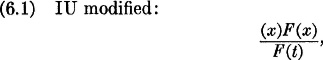
where t is a term.
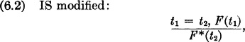
where t1 and t2 are terms.
ISC is modified similarly, but no other inference rules will be so modified. The extension of inference rules to accommodate terms is necessary for a systematic treatment of algebra, as was foreshadowed in Sec. 5.17. We shall refer to (6.1) and (6.2) by the old notation “IU” and “IS”, respectively.
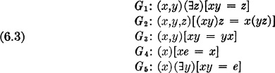
The second step in building the abstract theory is to add five non-logical axioms to the logic:
Group Axioms:
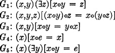
Since there is only one operational symbol involved in the system, it will be convenient to indicate the operation “xy” by simply writing “xy”. This is quite similar to the abbreviation of multiplication used in algebra. With this device the axioms are written
Two familiar interpretations of the abstract system are given by
| (6.4) | Let G be the set of all integers. Let ordinary addition be the binary operation in G. Interpret “e” as another name for zero. |
| (6.5) | Let G be the set of all positive real numbers. Let ordinary multiplication be the binary operation in G. Interpret “e” as another name for 1. |
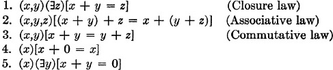
In either of these interpretations, the axioms become true statements in the interpretation. For (6.4), the axioms become the following five statements, which are easily recognized as true statements about the integers:
In the case of (6.5), the axioms become the statements:
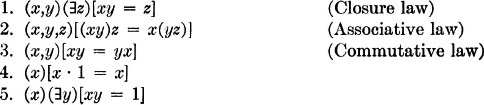
Observe that in the interpretation (6.5), the set G cannot contain the real number 0, since 0 has no reciprocal. Indeed, there is no real number x such that 0 · x = 1.
Any interpretation of the abstract system is called an Abelian group. If the commutativity axiom G3 is omitted from the system, then any interpretation of the resulting system is called a Group.
Examine the following sets of objects informally to see (a) which ones form groups and (b) which ones are Abelian groups:
1. A set consisting of just one element.
2. The set of real numbers with ordinary multiplication as the binary operation.
3. Negative real numbers with ordinary multiplication as the binary operation.
4. The integers with ordinary addition as the binary operation.
5. Integers except zero with ordinary multiplication as the binary operation.
6. The real numbers except zero with ordinary multiplication as the binary operation.
7. The set of translations in a plane with one translation following another as the binary operation.
8. The set of rigid motions (translations and rotations) in a plane with one rigid motion following another as the binary operation.
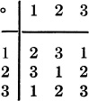
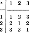
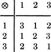
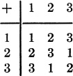
9. The set of numbers 1, 2, 3 with the binary operation defined by the table
10. The set of numbers 1, 2, 3 with the binary operation defined by the table
11. The set of rotations in a plane of an equilateral triangle ABC into itself, with one rotation followed by another as the binary operation.
12. The set of all powers of 2 with the binary operation ordinary multiplication.
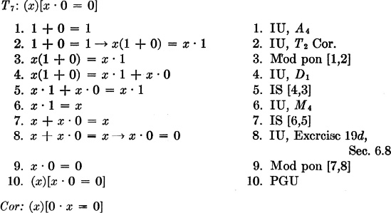
The third step in building the abstract group theory is to discover and demonstrate the lemmas and theorems that are logical consequences of steps one and two. We shall adopt an abbreviation in the application of IU and IE to axioms and previously proved theorems. For example, in deriving “ye = y” by IU from G4, we shall omit G4 as a step and merely write the result “ye = y”. Then in the analysis column will appear: “IU, G4”.
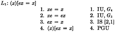
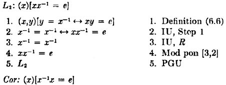
L1 can be regarded as a commutative form of G4.† It is a great convenience to have L1 since in all subsequent proofs, it will now be possible to use it to save three steps. For most of the theorems that follow, we shall follow the proof with an unproved commutative form of the theorem as a corollary.
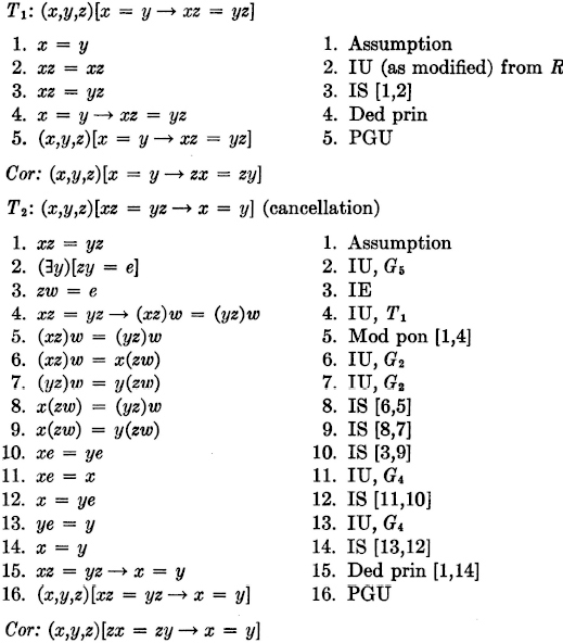
With the help of the cancellation theorem, G5 can be strengthened by showing that for each “x” there is not more than one “y” such that “xy = e”.
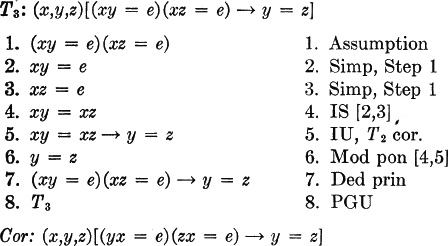
T2 and T3 together show that to each “x” there exists a unique “y” such that “xy = e”. Thus it makes sense to give a name to this uniquely determined object by the following definition:

One may regard “−1” as a singulary operation symbol that produces the term “x−1” when applied to “x”. The term “x−1” is called the inverse of “x”. It follows easily that
The next theorem shows that the individual constant e is unique in the sense that no other term has the property expressed in G4.
The next theorem shows that it is always possible to find a solution for an equation “ax = b” in an Abelian group.
EXERCISES
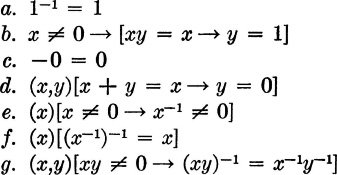
Write out a proof for each of the following statements:
† The reader will notice that we have abandoned the agreement made in Sec. 1.4 never to use a letter as the name of a statement. From now on, we shall use the symbol “G4”, for example, both as a symbolic translation of the axiom, and as a name for the axiom, and will no longer make a distinction by means of quotation marks.
The concept of an Abelian group1 is important to many branches of mathematics—algebra and topology, to name two. The Abelian groups that occur in the various branches of mathematics are interpretations of the foregoing abstract system. The development of the abstract system can be thought of as an investigation into the behavior of an arbitrary set of elements on which is defined a binary operation having certain natural properties. It is typical of modern mathematics to study such systems in the abstract, rather than via interpretations having additional properties, but properties that are irrelevant. In other words, if it is the behavior of binary operations that is of interest, then instead of investigating real numbers under addition, or rational numbers under multiplication, polynomials under addition or other existing structures, one strips away all irrelevant properties and attempts to see what happens in a system having just the properties of interest.
The investigation may be broadened by dropping some of the axioms, or adding some, or both. If axiom G3 is dropped, the resulting structure is that of a group. If G5 is dropped, the resulting structure is that of a semigroup. Group theory is often divided into the theory of finite and infinite groups. If a notion of limits is added to the group structure, the result is a theory of continuous groups. Abstract development of these notions is valuable because in a single investigation theorems are discovered and proved that have valid interpretations in many different branches of mathematics.
We have given two important examples of infinite Abelian groups in (6.4) and (6.5). We next give two examples of finite Abelian groups, and then take up the question: When are two interpretations essentially different?
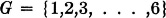
| (6.7) | Let G be the set of elements {1,2,3,4,5,6} with the binary operation taken to be multiplication modulo 7. |
To multiply x and y modulo 7, form the product xy under ordinary multiplication. Then divide xy by 7, and take the remainder to be the product modulo 7. That is,
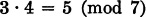
because 3 · 4 = 12 by ordinary multiplication, and on division of 12 by 7 the remainder is 5.
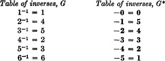
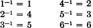
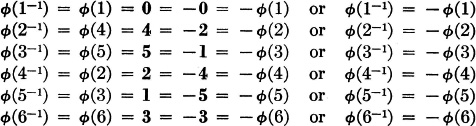
To verify that G is an Abelian group, it is necessary to check that the group axioms, considered as statements about multiplication mod 7 of the elements of G, are true. That multiplication mod 7 is defined for every pair of elements of G, and is associative and commutative follows easily from the corresponding properties of ordinary multiplication of positive integers. It is easy to see that 1 is the unit element (corresponding to e) of the group. To check for inverses, one observes, for example,

Hence, 2−1 = 4, and also, 4−1 = 2. The complete table of inverses follows, but it should be checked:
| (6.8) | Let H be the set of elements {0,1,2,3,4,5} with the binary operation addition modulo 6. |
To add mod 6, add in the usual way, then reduce the answer mod 6. It will probably be convenient here to symbolize the group operation by “+”, and to symbolize the inverse of “x” by “(—x)”. It is easy to see that “(x)[x + 0 = x]” and hence that the unit for this group is 0. The rest of the structure should be checked as in the previous example.
EXERCISES
1. A set of three objects can be ordered in six different ways. Any particular ordering is called an arrangement. The change from one arrangement to another is called a permutation. A permutation of three objects can be represented by

The numerals in this symbol refer to positions. The top row refers to the positions of the three objects before permutation; the bottom row refers to the positions the objects end up in after permutation. Thus, this permutation carries the object in the first position to the third position, leaves the object in second position fixed, and carries the object in third position to the first position. This permutation could also be written
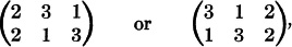
and in various other ways.
Let G be the set of all permutations on three objects. If one permutation is followed by another, the resulting effect can always be produced by a single permutation which is defined as the product of the two permutations.
a. Write out the six permutations of G.
b. Work out a scheme for finding the product of any two permutations, and check it by application to specific arrangements.
c. Which element plays the role of e?
d. Write out the inverse of each element.
e. Make up a multiplication table for the group. (Observe that the group is not Abelian.)
f. Find as many subgroups of G as you can. (A subgroup of G is a subset of elements H forming a group under the operation of G.)
g. Investigate the group of permutations on four objects.
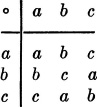
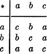
2. Let G be the set {A, B, C}. The operation is defined by the following table:
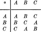
a. Which member plays the role of e?
b. Write the inverse of each element.
3. Let G be the set {1, —1,i, —i}, where i2 = —1. The operation is ordinary multiplication.
a. Which element plays the role of e?
b. Form a multiplication table for the group.
c. Write the inverse of each element.
We now consider the question: Are the Abelian groups G (6.7) and H (6.8) essentially different?
Any two interpretations of the same abstract system are “the same” in the sense that they both have all the properties expressed in the axioms of the abstract system. Every interpretation, however, has properties in addition to those of the defining system; hence, two interpretations can differ, and indeed, must differ in some sense in order to be distinguishable. We shall say that two interpretations are isomorphic if there exists a one-to-one correspondence between their respective elements that preserves the structures of the interpretations. We shall take up the meaning of the italicized phrases in this informal statement for the case of two Abelian groups, G and G*.
To say that there exists a one-to-one correspondence between G and G* means simply that to every x ε G there exists a unique corresponding element  (x) ε G*, and if x ε G and y ε G correspond to the same element of G* [that is, if (x) = (y)], then x = y. † Finally, for every x* ε G* there is an x ε G such that (x) = x*. Hence, under the correspondence , each element of G corresponds to a unique element of G*, and each element of G* corresponds to a unique element of G. (Finite groups having the same number of elements can always be paired in a 1-1 correspondence. For infinite groups, the matter is not so obvious.)
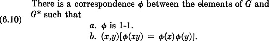
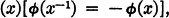
The structure of an Abelian group is determined by the multiplication table for its binary operation, the relation of each element to its inverse, and the properties of its unit element. To say that a correspondence preserves the binary operations is to say that if x (an element of G) corresponds to x* (an element of G*), and y corresponds to y*, then the product xy corresponds to the product x*y*, and this must hold for every possible choice for the elements x and y. Using the function symbol “”, we can express the property of preserving the binary operations neatly by

where it is understood that “x” and “y” name elements of G, and “(x)” and “(y)” name corresponding elements of G*. For the groups to be isomorphic, it must also be the case that
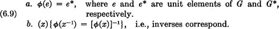
It can be proved that if the binary operations are preserved, then (6.9a) and (6.9b) also hold. Hence, isomorphism of groups is usually defined as follows:
Definition of Group Isomorphism (holds for groups as well as Abelian groups):
If G and G* are isomorphic, we write G ≅ G*.
As an example of isomorphic groups, we show that the group
with multiplication modulo 7, and the group G* = {0, 1, …, 5} with addition modulo 6, are isomorphic. We show the correspondence schematically:
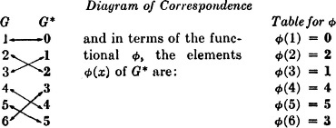
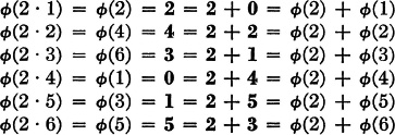
To help distinguish the groups, we symbolize the group operation in G by “·” and the operation in G* by “+”. Then, (1) = 0 shows that the unit elements correspond. We test preservation of inverses below (we indicate the inverse of x* in G* by —x*):
Then
So we have
and inverses correspond.
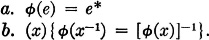
To check finally that

we proceed to check, for example, products formed with 2 (of G) as one factor:
The remaining products will be found to check similarly.
There are thirty-six different ways of setting up a one-one correspondence between the elements of G and G*. Of these 36 correspondences, or functions, some have the properties (6.10b) and some do not. It turns out that any function that does not make the unit elements correspond does not have the property (6.10b). Also, a function that makes 2 in G correspond to 1 in G* will not have the property (6.10b). However, the function  defined by the following table does have the required property:

Although it turns out that the functions and are the only ones having properties (6.10) for these groups, remember that the existence of one such function is enough to ensure isomorphism.
Now we prove that if has property (6.10b), all the structure is preserved.
T6: If is a correspondence between the elements of a group G and the elements of a group G*, such that

then
Two examples of isomorphic groups follow. Let
G be the set of integers with ordinary addition;
G* be the set of even integers with ordinary addition.
Then the 1-1 correspondence defined by the statement


The fact that G ≅ G* means that as far as ordinary addition is concerned, the integers and the even integers exhibit the same behavior. Let
G be the set of positive real numbers with ordinary multiplication;
G* be the set of real numbers with ordinary addition.
Then the existence of the 1-1 correspondence defined below demonstrates G ≅ G*
For

EXERCISES
Test the systems in each of the following exercises to see if the conditions (6.10a) and (6.10b) for an isomorphism can be satisfied:
1. G: the set of integers with ordinary multiplication
G*: the set of natural numbers with ordinary addition
2. G = {a,b,c} with the binary operation defined by the table:
G* = {1,2,3} with the binary operation defined by the table:
3. G = {2,4,6,8, … } with the binary operation ordinary addition
G* = {1,2,3, … } with the binary operation ordinary addition
4. Is there an isomorphism of the two systems of Exercise 3 if the binary operation in each case is ordinary multiplication?
5. G = {1,2,3} with the binary operation defined by the table:
G* = {a,b,c} with the binary operation defined by the table:
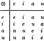
6. G = {a,b,c,d} with the binary operation defined by the table:
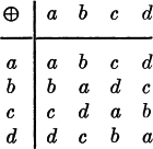
G* = {e,i,a,u} with the binary operation defined by the table:
1 For a good and accessible introduction to groups, see The Twenty-third Yearbook of the National Council of Teachers of Mathematics, “Insights Into Modern Mathematics,” chap. V, Washington, D.C.: National Council of Teachers of Mathematics, 1957.
† Recall that “x ε G”means: “x is an element of G”.
Elementary algebra has a more complex structure than that of the Abelian groups of the foregoing sections, since at least two distinct binary operations are required. Yet the group structure is to be found in elementary algebra, for the real numbers under addition form an Abelian group, and so do the real numbers (except zero) under multiplication. One way to set up an abstract system expressing the laws of algebra is to consider a universe having two distinct binary operations defined on it, with appropriate axioms to produce two Abelian groups. To connect the two groups operationally, it will be necessary to state an axiom concerning combination of the two operations. Interpretations of the resulting system are called fields.
The two operations will be symbolized by “+” and “·”. The symbols are borrowed from arithmetic and the operations are usually called simply addition and multiplication, even though they are entirely abstract operations, not to be confused with the operations of the same names in arithmetic and algebra. Two individual constants will be needed, and will be symbolized by “0” and “1”. We immediately adopt the abbreviation of writing “xy” for “x · y”.
Field Axioms:
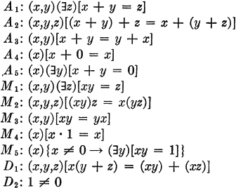
The first five axioms are just the axioms for an Abelian group. The next five axioms are also the axioms for an Abelian group, except for the restriction embodied in M5. Note that in applying IU to any axiom, 1 and 0 are legitimate values for obtaining substitution instances, even in the case of M5.
It is customary to call axioms A1 and M1 closure axioms; A2 and M2 associativity axioms; and A3 and M3 commutativity axioms. D1 is called a distributivity axiom; it connects the two field operations. We shall make the usual agreements about omission of parentheses in expressions involving both operations (see Sec. 2.9), and shall write “xy + xz” for “(xy) + (xz)” in what follows.
D2 is assumed for the purpose of ruling out the trivial interpretation consisting of a single individual. Without D2, the set consisting of the single element n would be a field if the operations were given by the table:

Inverses for the two operations may be defined as in the system for abstract groups. A5 and M5 establish existence of additive and multiplicative inverses, and the analogue of T3, Sec. 6.2, may be proved for each of the field operations to establish uniqueness of inverses. We shall not prove these analogue theorems, but state them as
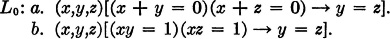
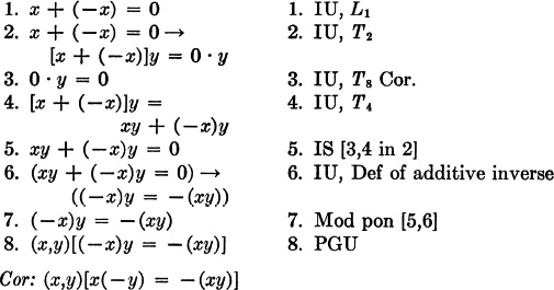
A5, M5, and L0 justify defining two inverse operators “ — ” and “−1” by means of the following equivalences:
Definition of Additive Inverse:

Definition of Multiplicative Inverse:1

The next lemma follows immediately. It is an analogue of L2, Sec. 6.2,
L1: (x)[x + (—x) = 0]
The proof is left as an exercise. A similar lemma about the multiplicative inverse has a slightly longer proof. We state it without proof:

A number of theorems can now be stated without proof since they have already been proved as theorems of the system for abstract groups of the previous section. The proofs for the present system go through in the same way with obvious notational changes.
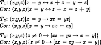
In fact, the analogue of T3 does not exist in group theory, but the proof of T3 is only a slight modification of the proof of T2, Sec. 6.2, and is left as an exercise. T3 expresses a cancellation law for multiplication, and T1 contains a cancellation law for addition.1
The next lemmas are useful in dealing with equations of the system.

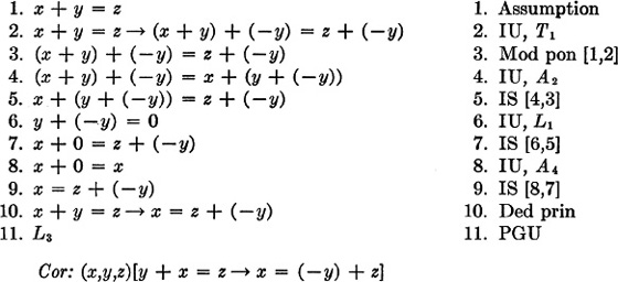
With some slight modification the next lemma is proved similarly:
1 The form of this definition entails some subtle difficulties that we do not pursue here. For a good discussion of the treatment of zero in definitions of division, see Patrick Suppes, Introduction to Logic, pp. 163–169. Princeton, N.J.: D. Van Nostrand Company, Inc., 1957.
1 These cancellation laws should not be confused with a student’s cancellation law well known to all mathematics teachers which states: “If a symbol appears twice on a page, cancel”.
An interpretation of the abstract system is a set F of objects having two operations defined on it. The abstract operations correspond with these operations defined on F. There must be two unit elements of F to correspond to the individual constants 1 and 0 of the abstract system. With the correspondences so determined, the axioms can be interpreted as statements about F; if they are true statements about F, F is called a field. Two examples follow.
The Field of Real Numbers:
| (6.13) | Let F be the set of real numbers. Take 0 and 1 as the unit elements, and ordinary addition and multiplication for the binary operations. |
All the axioms are recognizable as familiar properties of real numbers. Of course, the real numbers have other properties than those given by the axioms, or deducible from the axioms. For instance, the real numbers are ordered by an order relation (“ < ”), and there are infinitely many real numbers.
Other fields have their own special properties that distinguish them from the field of real numbers. An example is (6.14).
The Field of Integers Modulo 7 (From now on denoted by “F[mod 7]”):
| (6.14) | Let F be the set of numbers {0,1,2,3,4,5,6). Take 0 and 1 as the unit elements. Take for the binary operations addition and multiplication modulo 7. |
It is easy to see that field axioms A1 · · · A5, M1 · · · M5 are satisfied. Clearly D2 is satisfied; so there remains the check of D1.
Since there are only a finite number of substitution instances of D1 in this interpretation, we could check each one. This would entail checking 196 cases. It will be more economical of effort to show that D1 in the interpretation follows from the distributivity of the real numbers. Since we will need here to distinguish between addition and multiplication of real numbers, and addition and multiplication in our finite field, we distinguish these operations for the sake of this informal proof by using “  ” and “” to denote the operations in the finite field.
Now by definition, xy is the remainder obtained on dividing xy by 7. Hence,
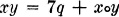
for some integer q, and
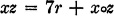
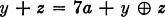
for some integer r. (Observe that both xy and xz are less than 7 by definition of remainder.) Then adding,

But,

for some integer s; so

On the other hand,
for some integer a; and so

Now,

So by substitution

But D2 holds for ordinary addition and multiplication of real numbers; so
Hence,

Now, both x(y z) and xy xz are remainders after division by 7; hence, it follows from the last equation that these remainders are equal. (If two numbers are equal, their remainders on division by 7 are equal.)
This field is finite and hence quite different from the field of real numbers. As will be shown later on, the field of integers modulo 7 cannot be ordered as can the real number field. However, F[mod 7] is a field, and one can expect to solve equations in it (simultaneous systems of equations included) and do many other of the same sorts of things that can be done with the field of real numbers.
Before proving further theorems of the abstract system, let us reiterate the purpose of these demonstrations. We are trying to show that certain statements in the system are theorems. That is, that the statements are logical consequences of the small set of axioms. As asserted earlier, we are not trying to convince anyone that the statements are true statements about numbers. One needs no convincing that the statements in a real-number interpretation are true. Perhaps conviction is not so certain in the interpretation (6.14), but in any event, we prove the theorems for formal reasons, and conviction or faith is not in question.
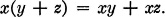
Numerous statements similar to T4 can be proved as consequences mainly of the associative and commutative axioms, with occasional use of D1. We give one further example.
EXERCISE
1. Show that subtraction is not an associative operation
a. By counter example in the field of real numbers,
b. By counter example, or other means, for the abstract system.
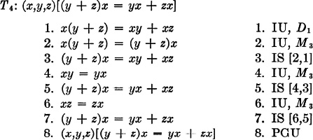
The proof of T5 is somewhat informal, since here, as in the sections on groups, we omit the statements of the axioms as steps in the proof. An unabbreviated demonstration of T5 would have, preceding our Step 1, a statement of A2. The degree of informality, or what is the same, the amount of abbreviation, permitted in proofs depends upon the purpose for carrying out the proof. As we pointed out before, a rigorous demonstration has the advantage that it is easy to check for validity since the definition of “demonstration” is relatively simple. A disadvantage of demonstrations is their excessive length. Informal proofs are usually shorter than demonstrations, but accurate description of what is meant by “proof” is much more complicated to state. Furthermore, errors in logic are less likely in demonstrations than in informal proofs. A good compromise is to consider any informal proof to be an abbreviation of a demonstration, where the types of abbreviations to be allowed are specified. The abbreviations may be of the logical forms of proof, as suggested in Sec. 3.10; or abbreviation may consist in omitting mention of certain specified theorems and axioms; or finally, the abbreviation may involve the notation, for example, the agreement to omit parentheses in “(xy) + (xz)”.
In any rigorous development of algebra from axioms, such as we have begun with the field axioms, we would not go on forever proving theorems as formally as we have. As the theory develops, abbreviations can be introduced systematically. The type of abbreviations and the timing of their introduction are a matter for good pedagogical judgment.
Algebra has a great advantage over geometry as a vehicle for teaching axiomatic structure. For not only is the required logical apparatus simpler, but rigorous demonstrations of the early theorems of algebra are far less lengthy than are demonstrations of the early theorems even of the miniature geometry, as a glance at the Appendix will show. Demonstrations of most theorems of Euclidean geometry are much longer than those of the miniature geometry. As a consequence, abbreviation of proof is much greater in plane geometry, and must come much sooner there than would be necessary in algebra. An important device for shortening proofs in plane geometry is to reason from the figure—while at the same time telling a student that he must not do this. Such devices and other abbreviations of proof are so numerous in plane geometry that it is extremely difficult to give a clear description of what a proof is. If a clear description of proof is not available, then no clear description of abbreviation of proofs is possible.
We list typical abbreviations with comments on their use in this chapter.
Logical Abbreviations |
Comment |
1. IU with major premise tacit |
1. Full use (Already discussed in this section) |
2. Multiple use of IS |
2. Generally full use (discussed below) |
3. Tacit use of commutativity, i.e., “AB” for “BA” |
3. Often used |
4. “ABC” for “(AB)C” and “A∨B∨C” for “(A∨B)∨C” |
4. Full use |
5. Discharge of an assumption by indirect proof |
5. Full use (discussed in Sec. 5.19) |
6. Logical substitution from a valid statement formula of equivalence, with the valid statement formula tacit |
6. Full use (discussed below) |
7. Modus ponens with major premise tacit |
7. Rarely used |
8. IS with one premise tacit |
8. Not used |
9. Conjunctive inference tacit |
9. Not used (will be used in Appendix) |
10. Simplification tacit |
10. Not used (will be used in Appendix) |
Multiple use of IS can be illustrated by modifying the proof of T4. Simply omit Steps 3 and 5. Then as the analysis for Step 7, write “IS [2,4,6 in 1]”. Omission of any one of the Steps 2, 4, 6 in proving T4 would be an example of abbreviation of Type 8.
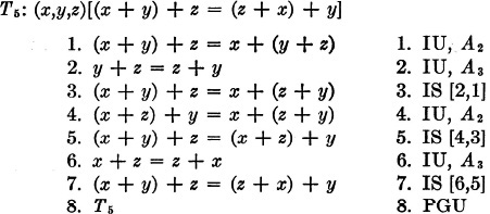
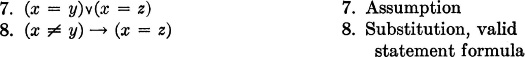
As an illustration of a Type 6 abbreviation consider that at Step 7 of a demonstration we have

and we want to obtain “x ≠ y → x = z”. A full demonstration would call for
We abbreviate as follows:
Field System Abbreviations |
Comment |
1. Omission of parentheses in mixed expressions (“xy + xz” for “(xy) + (xz)”) |
1. Full use (already discussed in this section) |
2. “x + y + z” for “(x + y) + z” “xyz”for“(xy)z” |
2. Used in interpretations, but not in the abstract system (discussed below) |
3. Associativity and commutativity tacit |
3. Used in interpretations, but not in the abstract system |
4. Use of cancellation theorems in form of derived inference rules |
4. Not used (discussed below) |
The expression “x + y + z” is not a term in the system (see Sec. 6.2). By agreement, however, it may be taken as shorthand for “(x + y) + z”. Extending the agreement, one may write “x + y + z + w” for “[(x + y) + z] +w”. It is then but a short step to the abbreviation of leaving the associative axiom for addition completely tacit. Such abbreviation is quite useful in algebra, and we may use it in interpretations of fields. We shall not use it in the abstract development, however, since to do so would obscure the role of Axiom A2. Similar remarks are of course possible about multiplication.
As an example of a Type 4 abbreviation, we might write
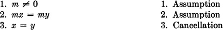
This is an abbreviation for

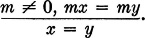
In effect, “cancellation” in the abbreviated version indicates use of an inference rule derived from T3, namely,
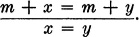
A similar inference rule could be stated for addition
There is no doubt that such inference rules are useful in algebra, and we shall sometimes use them without comment when working with interpretations of the abstract system, but never in the system itself.
A typical statement of an elementary algebra exercise might be

There are at least two distinct ways of regarding the problem. One may interpret the injunction “Solve the equation” as meaning transform the given equation by means of certain algebraic rules into an equation of the form “x = a number”. The problem is then successfully dealt with if the required activity is carried out to produce “x = 1”. Alternatively, one may interpret the problem to be: Find all solutions to the equation, which means, find all values for x that satisfy the equation. Then the problem is successfully dealt with if one discovers that 1 is the only such value.
Unfortunately, the words “solve” and “solution” are often used in both senses, and are thus ambiguous. The ambiguity is quite unnecessary. If the first interpretation is desired, the problem could be stated
Find an equation equivalent to “2x + 5 = 7” in
the form “x = a constant”.
Equivalence of equations would, of course, have to be understood. If the second interpretation is desired, the problem could be stated
Find all solutions (or roots) of “2x + 5 = 7”.
“Solution” or “root” would have to be understood as a value for x that satisfies the equation, i.e., yields a true substitution instance for the equation.
In practice, one usually finds the root of an equation by first reducing the equation to an equivalent equation of the form “x = a”, then clearly “a” is the only root. For the particular equation “2x + 5 = 7” we proceed as follows:
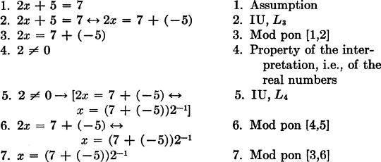
NOTE: If we want to make use of additional properties of real numbers, we may write the equation of Step 7: x = 1. So

It is well to pause here to see exactly what has been proved. The foregoing proof demonstrates

The statement (6.15) means that every true substitution instance of “2x + 5 = 7” is a true substitution instance of “x = 1”. While it is perfectly clear that substitution of “1” for “x” yields a true substitution instance of “x = 1”, we have not proved that this will yield a true substitution for “2x + 5 = 7”. In other words, we have not proved that 1 is a root of the original equation. In order to prove that 1 is a root of “2x + 5 = 7” we must prove

There are two ways of accomplishing the proof that 1 is a root. The easiest is to prove (6.16) directly from the addition and multiplication tables for real numbers. Another way is to prove

We leave the proof as an exercise. After (6.17) is proved, we use IU to get

and since “1 = 1” results by IU from Axiom R, we have (6.16) by modus ponens.
It is important to observe that while (6.15) does not mean that 1 is a root of “2x + 5 = 7”, it does mean that any root of “2x + 5 = 7” is a root of “x = 1”, and since 1 is the only root of “x = 1”, we have that 1 is the only possibility as a root for “2x + 5 = 7”. Hence (6.15) and (6.16) together establish that 1 is a root, and the only root, of “2x + 5 = 7”.
Thus, we see that when the elementary algebra student starts with the equation “2x + 5 = 7” and arrives by algebraic manipulations at “x = 1”, he has not found a root of the equation yet. The subsequent checking by substitution of “1” into the equation is a logical necessity, and not just for the purpose of guarding against error. Of course, for simple linear equations such as this, when one is able to infer “x = r”, it always turns out that r is indeed a root; so it is hard at this stage to bring home to the student the logical necessity for checking. It becomes easier when one has reached more sophisticated equations, where it is possible to infer “x = r” but r is not a root of the original equation.
It is worth noting that in the derivation, except in Steps 8 and 9, no properties of the numbers 2, 5, 7 were used that are not properties following from the uninterpreted field axioms. This suggests that it should be possible to prove as a theorem of our abstract system

The proof is left as an exercise. It turns out, as before, that [c + (—b)]a−1 is a root, and the only root, of “ax + b = c”.
Since T6 is a theorem of the abstract system, it can be used to solve equations in any valid interpretation. For example: Find roots of the following equation in the field F[mod 7],

Applying T6, by IU,

From the properties of F[mod 7],
so

and the required root is 5.
Normally one does not try to remember such theorems as T6 in an algebra, but solves simple equations like (6.18) by a combination of applications of axioms and cancellation theorems used in abbreviated form. Thus (6.18) could be solved by first multiplying both members by 2 to obtain

Then add 1 to both members of (6.19) to get

EXERCISES
Write out proofs for each of the following lemmas, theorems, or corollaries:
1. L0, page 198
2. L1, page 198
3. L2, page 199
4. T1, page 199
5. Corollary to T1, page 199
6. T2, page 199
7. Corollary to T2, page 199
8. T3, page 199
9. Corollary to T3 page 199
10. Corollary to L3, page 199
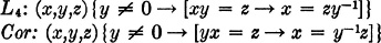
11. L4, page 199
12. Corollary to L4, page 199
13. (6.17), page 207
14. T6, page 207
Find the solutions of the following equations in a form analogous to that used on page 206:
15. 3x + (—5) = 7
16. 4x + 3 = x + 15
17. In F[mod 7], 3x + 2 = 4
18. In F[mod 7], 5x + (−3) = 2x + 6
19. Prove:
20. Prove: 
The next theorem is the basis for solving quadratic equations by the method of factoring.
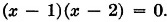
As an application of T8 in the field of real numbers, consider the problem of finding the roots of

We shall proceed informally. From the identity,

by IU and IS
Then by IU from T8,

So, by modus ponens,

and finally,

So, by the deduction principle and PGU,

It is easy to see that 1 and 2 are numbers yielding true substitution instances of (6.21). That is,
and
are both true. Clearly 1 and 2 are the only real numbers yielding true substitution instances of (6.21). Then from (6.22) it follows that there are no roots of (6.20) different from 1 and 2.1 Direct substitution in (6.20) will verify that the roots are indeed 1 and 2.
Certain errors of language and logic are frequently encountered in the treatment of the foregoing technique. It is quite common to find the solution to (6.20) expressed:

In the first place, a root of an equation is a number and is not another equation or statement function; hence, while the roots can be 1 and 2, they certainly cannot be x = 1 and x = 2. Second, the statement “x = 1 and x = 2” is surely false.
Proof:
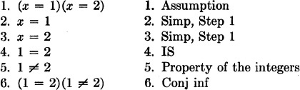
Of course, “x = 1 and x = 2” is intended to convey the information that 1 and 2 are values of x that satisfy x2 − 3x + 2 = 0. Since it is just as easy to convey the same information by a correct statement, statements such as (6.23) should be avoided.
Since T8 is a theorem in the abstract system, it is a true statement about any field, and can be used to solve suitable quadratic equations in, for example, F[mod 7]. Consider the solution of

in F[mod 7]. Then, informally,

So
Then, since

the roots of (6.24) are 1 and 2.
The set of numbers {0,1,2,3,4,5} with addition and multiplication modulo 6 is not a valid interpretation of the abstract field system (for example, M5 does not hold) and T8 is not a true statement about this set and its operations, as is shown by the counter example

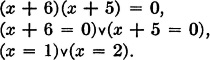
Thus T8 is not available for solving quadratic equations in the modulo 6 system. For example, suppose we attempt to solve the equation

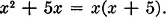
in the system modulo 6. It is easy to show the identity

and obtain by substitution

Now, lacking T8 for this system, we cannot deduce from (6.26)

and in fact neither (6.25) nor (6.26) implies (6.27), since both 0 and 1 yield true substitution instances of (6.25) and (6.26) but not of (6.27). In fact, the roots of (6.25) are 0, 1, 3, 4, but only two of them satisfy (6.27).
It is also worth noting that the quadratic polynomial “x2 + 5x” can be factored into two linear factors different from those of (6.26), i.e.,
Thus there is a second-degree polynomial in the system modulo 6 that has more than two distinct roots and more than one factorization into linear factors. Such a situation is not possible in a field.
The foregoing examples suggest that many of the basic theorems of algebra may depend only on field properties. Furthermore, however obvious T8 may seem, it expresses a basic and important property of elementary algebra.
EXERCISES
1. Prove the corollary to T7, page 209.
2. Fill in the details of the solution of the quadratic equation given on page 210.
Find all the roots of the following equations:
3. x2 + 4x + (−5) = 0 in F[mod 7]
4. x2 + 5x = 0 in F[mod 7]
5. x2 + 4x = 0 in the system modulo 6
6. x2 + 3x + 2 = 0 in the system modulo 6
7. x2 + 2x + (−1) = 0 in F[mod 3]
8. 2x2 + 3x + 4 = 0 in F[mod 5]
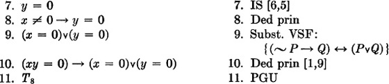
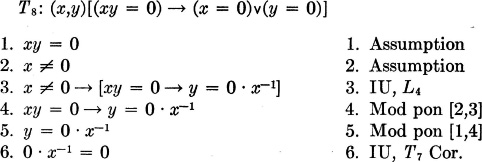
9. Prove: (x,y)[xy ≠ 0 → (x ≠ 0)(y ≠ 0)]
1 Perhaps it is easier to understand the uniqueness of roots by considering a statement equivalent to (6.22): (x) {(x ≠ l)(x ≠ 2) → x2 − 3x + 2 ≠ 0}.
The inverse operations of subtraction and division may be introduced into the abstract system by definition.
Definition of Subtraction:

Definition of Division:

In the definition of subtraction, the symbol “ — ” enters ambiguously. In “x — y” the symbol “ — ” is used to denote the binary operation of subtraction, but in “(— y)” the same symbol is used to denote the singulary operation of negation. While the two operations are closely related, they are not the same, and strictly should be denoted by different symbols. It is customary in algebra, however, to use the same symbol for both operations and to depend on context to determine which operation is meant. The rule to follow is:
a. When “ — ” occurs between two terms, the binary operation of subtraction is indicated.
b. When “ — ” occurs before a single term, the singulary operation of negation is indicated.
Such expressions as

are not properly formed and will not be used as abbreviations. On the other hand, the expression
is customarily used as an abbreviation for
and

is an abbreviation for

Such mixed expressions are not ambiguous since it is understood that association is to the left. So, for instance, (6.28) is our abbreviation for (6.29), while the following are not:

All the above are familiar conventions of algebra. They are practical abbreviations and not hard to learn. It seems unfair, however, to expect the algebra student to learn them without some explicit exposition by the teacher. Many of the usual errors committed by algebra students result from confusion about these conventions.
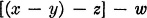
With the foregoing definitions, it is easy to deduce properties of subtraction and division. We list some without proof:
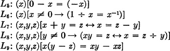
The equation in two variables

can be thought of as an equation in the field of real numbers if the universe of individuals is limited to the real numbers. Various substitution instances of (6.30) are
The false substitution instance (6.31a) is obtained by replacing “x” by “2” and “y” by “11” in (6.30). It is convenient to say that substitution of “(2,11)” in (6.30) yields (6.31a), where we agree that the first member of the ordered pair is substituted for “x” and the second member of the ordered pair is substituted for “y”. Similarly, (7,3) yields (6.31b), (3,7) yields (6.31c), and so on.
We call any ordered pair a solution of (6.30) if it yields a true substitution instance of (6.30).
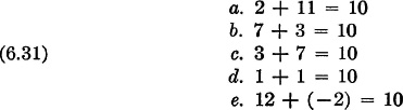
The injunction: Solve the system:
has the same ambiguity of meaning as for the case of a single equation in one variable. We shall interpret the injunction to mean
Find all ordered pairs of numbers yielding true substitution instances for “(x +y = 10) and (x — y = 6)”.
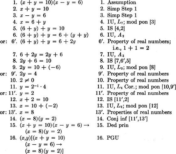
First we prove

The proof will be abbreviated by multiple use of IS and by suppressing major premises of modus ponens. The multiplication and addition tables for integer numbers are assumed known.
It is clear that (8,2) is the only ordered pair that yields a true substitution instance of
Hence, if the original pair of equations has any solution, it is (8,2). Verification is by direct substitution:

The proof of (6.33) is long even with the abbreviations. The object in presenting it is to show how the familiar procedure for solving the system (6.32) depends upon abstract field properties, and incidently to point out those spots where additional special properties of the real numbers are needed.
If one merely wants to find a solution for the system (6.32), the best way is to guess and check the guess; or if some sort of derivation is required, one would omit any mention of associative and commutative properties and perhaps write down Steps 2, 3, 4, 5, 8, 9′, 11′, 12, 13′, and then check the solution suggested by 11′ and 13′.
The proof of (6.33) suggests that in solving a system of simultaneous equations, one is really starting from a conjunction of the two equations. One derives a simple conjunction of the form “(x = a)(x = b)”. This establishes uniqueness of the solution. Then one checks to establish existence of (a,b) as the solution.
There are, of course, systems of linear equations having no solution. The proof, in such a case, is quite straightforward. Consider the system
We start by assuming the conjunction

and proceed informally to get the separate equations by simplification. Then

and by substitution of (6.36) in the first equation of (6.34)
which yields

But 6 ≠ 10, so we have a contradiction, and the logical negation of (6.35) is established. Then by PGU

or by conversion of quantifiers

The proof is quite straightforward, and does not require geometric arguments leaning on parallelism. We do not want to discount the value of geometric interpretations in teaching algebra, but merely want to point out that the inconsistency of the system (6.34) is a fact of the real-number field, quite independent of geometric notions.
The procedures for solving systems of equations in the real-number field should be effective in any field, taking into account the addition and multiplication tables of the field. For example, consider the following system in F[mod 5]:
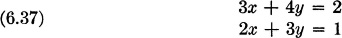
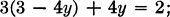
We solve the system (6.37) informally, and start by multiplying both members of the second equation by 3 to obtain

Then, by L7,

and, by substitution in the first equation of (6.37),
or
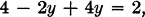
or

Then, adding 1 to both members, and then multiplying both members by 3,

Substitution in (6.38) yields

Thus the system (6.37) implies the system
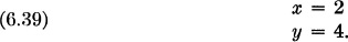
The only solution of (6.39) is clearly (2,4), and direct substitution in (6.37) shows that (2,4) is a solution, and hence the only solution of (6.37).
EXERCISES
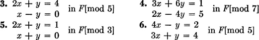
Write out a proof analogous to (6.33) for each of the following systems of equations:

Solve each of the following systems of equations in the indicated field:
7. Show that if division is associative in a field, then

can be proved. Then find a field having this property.
8. Prove: (x,y,z){(x — y) + z = x + (z — y)}.
9. Prove: In the field of real numbers

One of the mysteries of elementary algebra is this: Why is it that (—2)(—2) = +4? Removing the mystery from this question poses problems to the teacher because the student normally builds his conception of numbers by abstracting from many different interpretations of numbers. Unfortunately, such interpretations of positive and negative numbers as credits and debits, or temperature, etc., that work so well in teaching addition and subtraction of signed numbers are not so satisfactory for dealing with multiplication of signed numbers, particularly for the case of (—2) (—2).
In fact, the answer is to be found in formal considerations. Essentially, (—2) (—2) = +4 because it is defined that way. Still, one can ask why is the product defined this way rather than as —4, or 7, or  or
or  ? To answer this, we must consider how the integers are themselves defined.
The natural numbers 1, 2, 3, … with ordinary addition and multiplication have all the properties expressed in the field axioms A1, A2, A3, M1, M2, M3, M4, D1. Subtraction and division can be defined for some pairs of natural numbers, but not for others. One can now try to extend the natural numbers to a larger system in which subtraction is always defined by creating some new numbers to serve as differences such as 1 — 3, 3 — 10, etc., which are not defined for natural numbers. The requirement that subtraction be always possible is equivalent to the requirement that A4 and A5 hold for the system. Of course, one wants the new system to satisfy all the axioms satisfied by the natural numbers. But with all these axioms satisfied, it is possible to prove

where the “ — ” denotes the negation operation as defined for fields.
The procedure for extending the natural numbers might then be:
1. Assume an integer denoted by “0” satisfying A5 and D2.
2. Call the natural numbers positive integers, and assume for each positive integer x a corresponding negative integer, to be denoted (for the moment) by “ ”, with the property that = —x. [Remember, “ — ” denotes the negation operation.]1
If addition and multiplication of the signed numbers are now defined in the usual way, the resulting system will be found to satisfy all of the required axioms. In particular, one easily proves, — = x.
It is worth noting that the property that the product of two negative integers is positive is in a sense a special case of (6.40b), which is a statement about all integers. By definition of  and
and  , we have = (—2) and = (—3); hence from (6.40b) we obtain: · = 2 · 3. But from (6.40b), one also can obtain: (—)(—3) = · 3 and (—)(—) = · . In fact, (6.40a) and (6.40b) can be proved as consequences of A1 to A5, M1 to M4 and D1, D2 without any notion of positive and negative numbers. As we are about to show, (6.40a) and (6.40b) are theorems of the abstract field system, and hence express properties of all fields. Yet in the field F[mod 5] the notion of positive or negative numbers is meaningless (see Sec. 6.14).
We now prove (6.40a) and (6.40b) as Theorems 9 and 11 for abstract fields.

Proof: (Abbreviation through multiple use of IS)
1 A more elegant method for extending the natural numbers is to deal with a set whose elements are ordered pairs of natural numbers. A short account of this method can be found in: The Twenty-third Yearbook of the National Council of Teachers of Mathematics, “Insights Into Modern Mathematics,” chap. II, Washington, D.C.: National Council of Teachers of Mathematics, 1957.
The field of real numbers has all the properties expressed in the axioms and theorems of the abstract field system, but has other properties that are not deducible from these field axioms. Among these are:
a. The field has infinitely many elements.
b. There exist real numbers that are not the sum of two squares, e.g., —4.
c. The field contains a proper subfield, e.g., the field of rational numbers.
d. The real numbers are ordered by the relation “ < ” (less than).
Since the field F[mod 5] has none of these properties, it follows that none of the properties a, b, c, d are deducible from the field axioms.
It is not hard to verify that F[mod 5] does not have properties (a), (b), (c). Indeed, it is obvious in the case of (a). As for (b), in F[mod 5] one can write
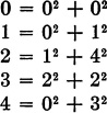
Hence, every element of the field is the sum of two squares.
In order to check property (c), we must first define subfield. A subfield H of a field F is a subset of F that forms a field under the operations of F. H is called proper if H is not the same as F. Now F[mod 5] contains no proper subfield, because any subfield would have to contain the unit elements 0 and 1, and hence would also (by A1) have to contain 1 + 1, and hence 2 + 1, and 3 + 1. That is, any subfield of F[mod 5] contains all the elements of F[mod 5], and is thus not a proper subfield.
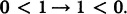
To show that F[mod 5] cannot be ordered, consider how 1 and 0 would be ordered, if this were possible. Since 1 ≠ 0, we should expect either that 0 < 1 or that 1 < 0, but not both. Suppose 0 < 1. Then adding to both members (mod 5 of course) should preserve the inequality in the same direction. Repeating this procedure five times yields the inequalities

The last four of these inequalities together imply that 1 < 0. So we have
Similarly it can be shown that
so finally
Since this result does not accord with what we expect of an order relation, we conclude that F[mod 5] cannot be ordered.
The foregoing discussion made tacit use of several properties of an order relation. We now state the properties formally as axioms. These axioms, added to the axioms for an abstract field, yield the axioms for an abstract ordered field. Any interpretation of the resulting abstract system is called an ordered field. The real numbers form such an ordered field, but as we have seen, F[mod 5] does not. Indeed, for all positive primes p, F[mod p] is not ordered.
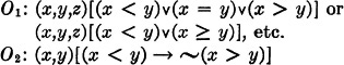
The Order Axioms [“x < y” is read “x is less than y”]:

The axioms O1 and O2 together express the trichotomous property of “ < ”, for from them it will be possible to prove (see T18) that the conditions “x < y”, “x = y”, “y < x” are mutually exclusive.
O3 expresses the transitive property of “<”; O4 and O5 connect the order relation with the binary operations and permit the usual manipulations of inequalities.
The order axioms express familiar properties of the order relation in the field of real numbers. We proceed to prove some theorems of the abstract ordered field system. In particular, we shall show that it makes sense to talk about positive and negative elements in any ordered field, “x is positive” will be interpreted to mean “0 < x”, and “x is negative” to mean “x < 0”. We do not introduce any new symbol to indicate a positive or a negative element; “+” always denotes the field operation of addition, and “ — ” either the binary operation of subtraction, or the singulary operation of negation, depending on context.
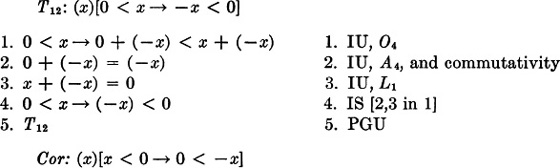
One can interpret T12 to mean that if x is positive, then — x is negative; and the corollary to mean that if x is negative, then — x is positive.
By repeated applications of O4, it can be proved that

The proof is left as an exercise.
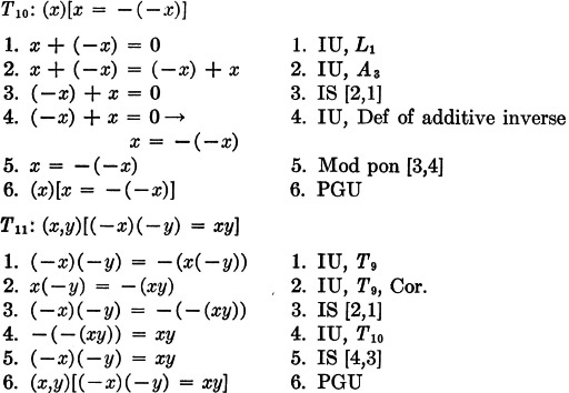
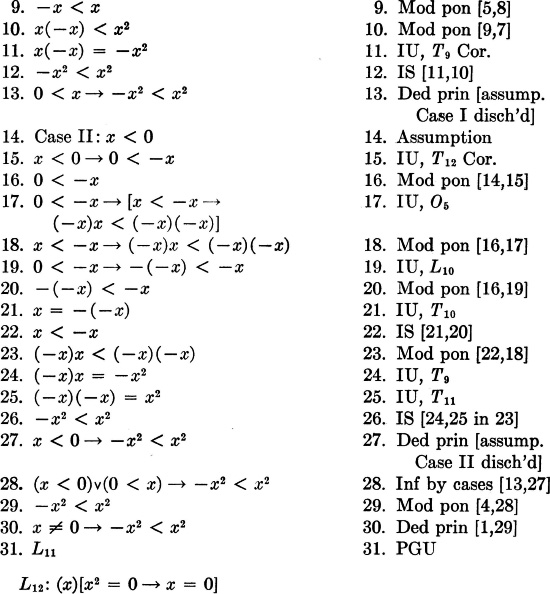
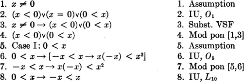
The next lemmas and Theorem 14 establish that in any ordered field, every square is positive except 02.
L10: (x)[0 < z→ —x < x]
Proof is left as an exercise.
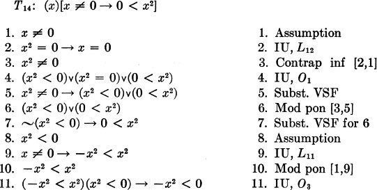
L11: (x)[x ≠ 0 → —x2 < x2]
Proof is left as an exercise. (Use T8.)
Since 1 = l2, it follows immediately from T14 that 1 is positive. From this result and T12 it follows that —1 is negative, hence,
T15:0 < 1
Cor: —1 < 0.
Theorems T12, T14, T15 provide another means for proving that F[mod 5] cannot be ordered. For, suppose it is ordered. Then, by T15, 0 < 1 and, from T12, 4 < 0 (since —1 = 4 in this field). This result conflicts with T14,since 4 = 22.
The same theorems allow us to prove that the field of complex numbers is not an ordered field. Suppose the complex numbers are ordered by a binary relation “ < ” satisfying the order axioms. Now the multiplicative unit for the field is 1 + 0 · i or 1. Hence by T15, 0 < 1 and by the corollary —1 < 0. But in this field i2 = —1; hence i2 < 0, and by T14, i2 < 0. From these results a contradiction is easy to deduce, and it follows that the complex numbers cannot be ordered. This is not to say that no sort of ordering can be introduced into the complex field, but whatever order relation is established, it will not satisfy all the axioms O1 to O5. One might, for instance, define

The relation  has some of the usual order properties, but not O1, for example.
In an ordered field, the connection between order and difference is easily established:

The theorem follows from O4 and the definition of subtraction,
1. Prove: T12 Cor., page 222.
2. Prove T13, page 222.
3. Prove L10, page 222.
4. Prove L12, page 223.
5. Prove T16, page 224.
6. Show that F[mod 7] cannot be ordered by finding two numbers whose squares add up to —1 and then proving this is a contradiction.
7. Write out an abbreviated proof of T14 that could be understood without knowledge of symbolic logic.
Abbreviations involving the symbols “ > ”, “ ≤ ”, “ ≥ ” are quite useful:
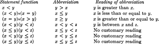
With these abbreviations, the trichotomy axioms O1 and O2 would be written
and O3 becomes

We shall use these abbreviations in the next theorem, and freely from now on.
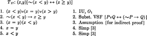
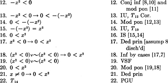
This theorem not only gives a useful form for “ (x < y)” but the internal indirect proof, Steps 3 to 10, shows that the cases “x = y” and “x < y” of O1 are exclusive. Clearly it follows that all the cases of O1 are mutually exclusive.
We could go on to prove equivalences expressing negations of “x > y”, “x ≥ y”, “x ≤ y”, but in fact they are all contrapositives or abbreviated forms of T17. Thus, when we need to negate any of the foregoing, we shall refer to T17.
The remaining theorems of this section are stated without proof. They express familiar properties of real numbers that are properties of any ordered field.
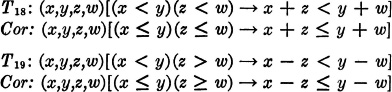
Observe that “→” may not be replaced by “↔” in T18, T19.
EXERCISES
1. Verify that the relation  defined for complex numbers, page 224, does not satisfy all the order axioms.
2. Prove T18.
3. Prove T18 Cor.
4. Prove T19.
5. Prove T19 Cor.
7. Prove T21, page 226.
8. Prove T22, page 226.
9. Prove: (x,a,b,c)[(x < a + b)(b < c) → x < a + c].
10. Prove: (x,y){(x ≠ 0)(y ≠ 0) → [x < y → x−1 > y−1]}.
11. Verify informally that the rational numbers form a proper subfield of the real numbers.
† A very common abbreviation for “(x < y)” is “x  y”.
y”.
The successful algebra student ultimately comes to understand the order relation in the real numbers. He understands that “a” (or even “+a”) can have negative substitution instances, and that “ —a” can have positive substitution instances. He is familiar with the interpretation of real numbers as points on a line, with “a < b” interpreted as “a to the left of b”. He probably has a workable concept of the distinction between subtraction and negation. These concepts are quite sophisticated compared with those he acquired when first approaching integer operations. For example, the concept of +2 and —2 as different aspects of 2 ultimately is replaced by the concept of +2 and —2 as integers that are negations of each other.
Generally, the language appropriate to the more sophisticated concepts will be different from the language used in the initial approach. In this initial treatment of integer operations, the teacher wants to build on his students’ knowledge of natural number operations and relations. Consequently, operational rules for integers are stated in terms of natural-number operations and the natural-number order relation as far as possible. One of the rules for addition of integers is often condensed into the statement
| (6.41) | To add two integers of unlike signs, take the difference and attach the sign of the larger. |
A little analysis of (6.41) shows that the language is quite poor. Let us apply (6.41) to obtain the sum of the integers +5 and —7. To begin with, +5 and —7 do not have unlike signs, it is the names “+5” and “ —7 ” that have the unlike signs. The connection between the signs and the integers is just an accident of the method of naming the integers. What are the signs of “ —(—5) ”, “+(5 — 12) ”, for example? It appears that (6.41) is a statement concerned with a particular way of representing integers. To go on with the rule, one now has to “take the difference”, but clearly not the difference of +5 and —7, but of 7 and 5. At this early stage, the student probably doesn’t distinguish between “the difference of 7 and 5” and “the difference of 5 and 7”, so he gets the difference 2. The larger of 5 and 7 is 7, so he attaches a “ — ” to the name “2” to get “—2” and the answer —2. Of course, it is the larger of 5 and 7 that is in question here, and not the larger of +5 and —7 which is what (6.41) really says to consider.
One of the troubles with (6.41) is that the antecedent of difference and larger is not the two integers. What is needed is some convenient name for the positive integer (or, if one likes, the natural number) associated with each integer. Thus, in applying rule (6.41) to the sum of +5 and —7, one operates with +5 and +7 (or 5 and 7) which are sometimes called the numerical values of +5 and —7, respectively.
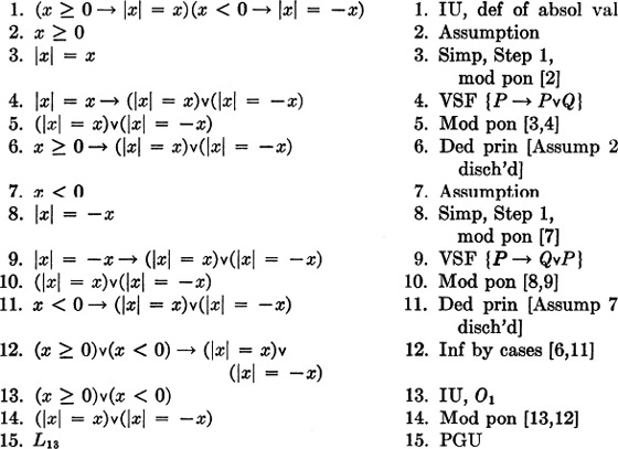
The term “numerical value” in this context is largely a term confined to elementary or secondary mathematics. It is virtually never used in higher mathematics, where the term “absolute value” is used instead. The absolute value of x is denoted by “|x|” and can be defined for any ordered field as follows:
Definition of absolute value (numerical value):

Note that “ — ” indicates the negation operator in (6.42). Statement (6.42) may be paraphrased:
If x is positive or zero, the absolute value of x is just x, and if x is negative, then the absolute value of x is the negation of x.
Using this notion of absolute value, (6.41) may be restated:
To form a name for the sum of a positive and a negative integer, find the absolute value of the difference of their absolute values. Then attach a “ — ” or a “+” sign according as the absolute value of the negative integer is greater than, or less than, the absolute value of the positive integer.
The statement is correct, but a pedagogical horror. An altogether simpler statement is:
To add a positive and a negative integer, from the integer of larger absolute value subtract the negation of the other integer.
For this rule to be effective, the student must know how to subtract —2 from —5, and —7 from —12, etc., but not, for example, —12 from —7.
However the language problems are solved in the statements of these rules, the rules are intimately concerned with the order relation among positive numbers. Where the language used at this stage is loose, the student is likely to acquire a deep down belief that —7 is greater than +5, etc. In some students this belief dies hard.
EXERCISES
1. Write out a set of rules for calculating (a) sums and differences of integers; (b) products of integers.
2. Give a geometric interpretation for |x — y|, where “x” and “y” denote real numbers.
3. Graph the equations:
a. y = |x|
b. y = |x + 2|
c. y = |x — 2|
d. y = |x2 — 3x + 2|
4. Describe informally the relation of the graph of y = f(x) to the graph of y = |f(x)|.
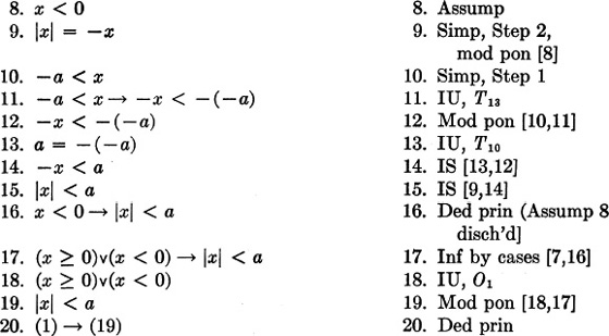
The further the student goes in many branches of mathematics, the more important the ability to handle inequalities becomes. For example, in elementary calculus one needs the theorem
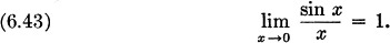
In the language of symbolic logic (6.43) can be written

While one does not attempt a very formal proof of such a complicated statement in elementary calculus, the mathematics student must ultimately be able to prove such statements, and this requires an ability to handle inequalities involving absolute value symbols. It is just at this stage that some students reach their limit in college mathematics. It is safe to say that the more acquaintance the student has with inequalities and the concept of absolute value the better equipped he is for higher mathematics. The high school student bent on pursuing a mathematics or science program in college should certainly have the opportunity to start this acquaintance with inequalities in advanced algebra, if not earlier.
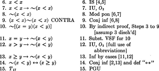
The lemmas and theorems that follow hold in any ordered field.

The proof follows easily from the definition of absolute value, O1, and the VSF “(P → Q)(P → R) → Q∨R”, but we give a proof, without assuming the VSF, which is typical of the proofs by cases needed for dealing with inequalities.
The next three lemmas are proved in much the same way; the proofs are about the same length, and are left as exercises.
L14: (x)[|x| ≥ 0]
L15: a. (x)[|x| ≥ x]
b. (x)[|x| ≥ —x]
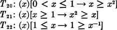
The next theorem and its corollaries state important equivalences:
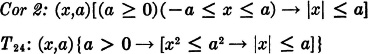
T23: (x,a)[(a > 0) (—a < x < a) ↔ |x| < a]
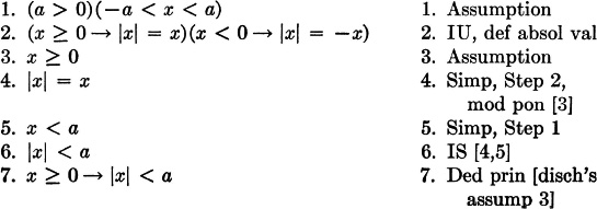
This proves half of the desired equivalence. The other half is left as an exercise.

To prove the corollary, first find a substitution instance for T23 by substituting “x — a” for “x” and “b” for “a”.
Proof: (contrapositive form)
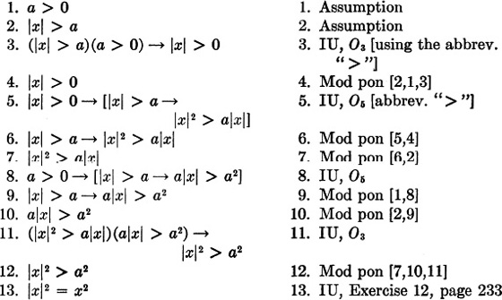
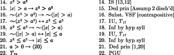
Cor 1: (x,a){a > 0 → [x2 > a2 → |x| > a]}
Cor 2: (x,a){a > 0 → [x2 ≥ a2 → |x| ≥ a]}
Cor 3: (x,a){a > 0 → [x2 = a2 → |x| = a]}
In the field of real numbers, the symbol  is so defined that if “a ≥ 0” then
  is true. For example,
  and
and  . Hence, in the real number interpretation, T24 can be written

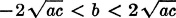
Indeed, an even simpler version is

With T23, T24, and the above result, several types of inequality problems associated with quadratic equations can be dealt with as easily as one solves simple equations. For example,
PROBLEM: Find the necessary and sufficient conditions on the real coefficients a,b,c with a ≠ 0, so that the roots of ax2 + bx + c = 0 are imaginary.
We assume it known that the roots are
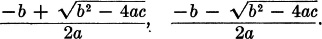
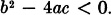
Assume both roots imaginary. Then
Or, using T16 or O4,

Now, since 0 ≤ b2 (easily from T14), it follows that 4ac > 0 and T23, Cor. 1, applies to yield

On the other hand, if we like, using T22
is the necessary condition.
To prove the condition sufficient, one would have to reverse all steps. This can be done using T22 and T23, Cor. 3.
EXERCISES
1. Prove L14, page 230.
2. Prove L15(a), page 230.
3. Prove L15(b), page 230.
4. Prove the other half of T23, page 230.
5. Prove T23 Cor. 1, page 231.
6. Prove T23 Cor. 2, page 231.
7. Prove T24 Cor. 1, page 232.
8. Prove T24 Cor. 2, page 232.
9. Prove T24 Cor. 3, page 232.
10. Prove: (x)[|x| = 0 → x = 0].
11. Prove: (x)[|x| = |—x|].
12. Prove: (x)[x2 = |x|2].
13. Prove: |0| = 0.
14. Prove: (x)[x2 ≥ 0] (very short proof).
15. Prove: (x,y)[x2 + y2 ≥ 2xy] (HINT: Use T14).
16. Abbreviate the proof of T24, and then write it out without using the symbolic language.
17. Prove: |ab| = |a||b|.
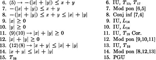
Early in the calculus, one needs the relations
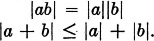
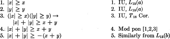
The equality is easy to establish and is left as an exercise. The inequality follows from L14, L15, T18, T23:
T25: (x,y)[|x + y| ≤ |x| + |y|
Sometimes a student first encounters the notion of a limit briefly in plane geometry. There may be further brief encounters in trigonometry and analytic geometry, but it is in calculus that the notion is first systematically exploited. From this time on, as long as he studies mathematics, his notion of limit will broaden and deepen. In the early stages, calculus is mainly concerned with limiting processes involving real numbers, and makes heavy use of the ordered field properties of the foregoing sections, although further properties of the real numbers are also needed.
A basic notion is that of limit of a sequence. For this discussion, a sequence is a real valued function defined over all the positive integers. We symbolize a real sequence by “ {An} ”, where “ An” denotes the value of the function for the positive integer n.
A particular sequence can be described in many ways, but most commonly by showing how to compute An for each n; for example (in this example, and in what follows, “n” is reserved to denote positive integers),

This sequence has for its first five terms
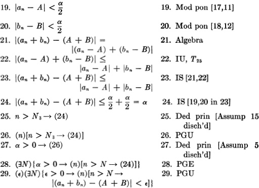
By the limit A of a sequence {An}, we mean, loosely, a real number A such that all but a finite number of terms of the sequence are arbitrarily close to A. More precisely

where we limit the values for the variables “n” and “N” to positive integers.
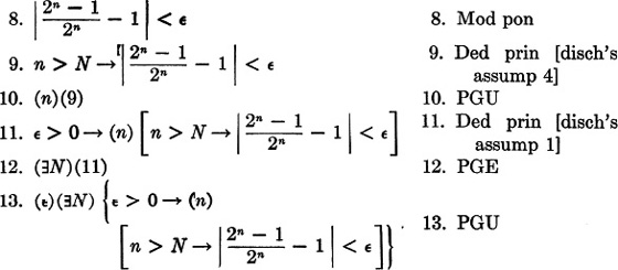
In this definition,  is a measure of the closeness of An to A, and N is a measure of how far out to go in the sequence so that terms beyond AN will be close enough to A. Let us prove that if
then lim An = 1. Here, we must make |An — A|, or in this case
small. Now
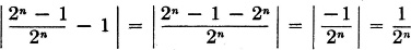
and
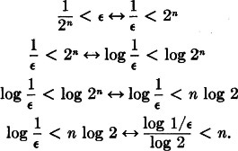
So for arbitrary > 0, we should choose
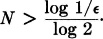
It is a property of the real numbers that any real number is exceeded by some integer. We now have the ingredients to prove that the limit of the sequence is 1.
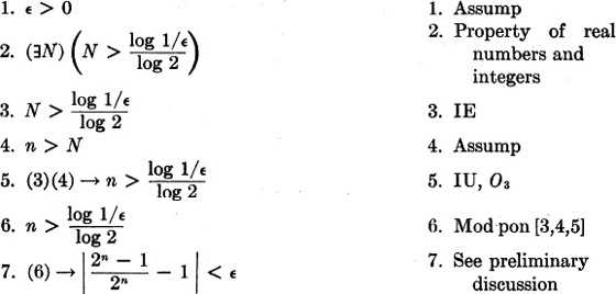
This proof is comparatively informal. Much of the abbreviation occurs at Step 7. To establish Step 7 formally would involve formalizing the preliminary discussion by means of theorems and axioms of foregoing sections. It is worth noting that it is just Step 7 that is peculiar to the given sequence, and really is the essence of the proof. The rest of the steps are common to all such proofs of the limit of a sequence. It is also worth commenting upon that it is just the relation of Step 7 to the rest of the proof that seems to cause the most trouble for beginning students.
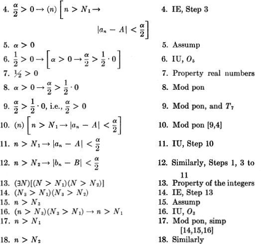
As a last example, we present a standard proof that makes use of T25.

What we need to make arbitrarily small here is
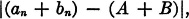
which may be written

and, by T25,

Since both terms on the right of this inequality can be made arbitrarily small by definition and the hypotheses, we can see our way clear to a proof:
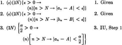
Observe that because of restrictions surrounding IE it is necessary to choose N1 and N2 independently in Step 4 leading to 11, and the corresponding step (tacit) that leads similarly to Step 12.
EXERCISES
1. Prove: lim bn = 0, where 
2. Prove: 
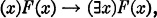
The symbols used for individual variables in mathematics are always used in a restricted way. The “x” and “y” of algebra are generally restricted to values in some class of numbers, usually the real or the complex numbers. The statement

is taken to assert the truth of all substitution instances, with the understanding that symbols substituted for the variables are numerals, not names for monkeys or other such objects. Sometimes one asserts that the universe of individuals consists of real numbers, or of complex numbers, and so on. It is very common, however, to make statements whose substitution instances involve several different classes. In algebra, for instance, one might write

where it is desired that the coefficients a,b,c are real numbers, but x may be complex.
In plane geometry, most theorems involve statements about points and lines. It is very convenient to make the notational agreement that certain letters will be used to denote points, and certain other letters will be used to denote lines. This constitutes a valuable agreement, and is handled in the logic by a formal agreement.
Suppose one wished a formal expression for the general statement
(6.44) If a point is on a line, then the line is on the point.
Then the translation for (6.44) is written

which may also be written:

In any development of geometry, every axiom or theorem will involve the predicates “P” and “L”. It will be a great convenience to make the following abbreviation agreement (where “F” is some unspecified predicate):
Agreement for Restricted Quantification:1

where lower-case Latin letters, early in the alphabet, are to be reserved for abbreviation (a), and lower-case Greek letters are to be reserved for abbreviation (b).
With agreement (6.46a) we may abbreviate (6.45) as

and, using agreement (6.46b), as

The formal advantages of (6.47) over (6.45) are clear.
For existential quantification we agree2

With these agreements, we may translate
on every line is at least one point,
as

Without the agreements (6.46) we would have to write (6.48) as

or perhaps,

So far, we have made agreements for abbreviating quantified statements. We must examine how IU and IE behave with these agreements. Clearly, by IU, from
we can get
It is natural to expect to apply IU to

and obtain

However, one would also expect to apply IE to

to obtain

with, of course, the usual restrictions on b in future applications of PGU. The difficulty here is that (6.49) is an abbreviation for

and (6.50) is an abbreviation for

Now, (6.51) and (6.52) are quite different. If one is to use IU and IE in this way, it seems that one will have to remember where such a formula as “F(a)” comes from, in order to know what its unabbreviated form is. Observe that, while it is a simple thing to prove
it is not possible to prove

Let us try, using unabbreviated forms. We want to demonstrate
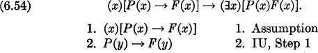
At this point we are stuck, because there is no way of deducing “P(y)”, which is necessary at this point. Suppose, however, that there is an axiom of the geometry stating the existence of points,
Axiom: (∃x)P(x).
Then it is possible to prove (6.54) as follows:
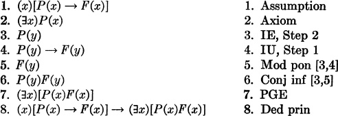
Thus it is not possible to prove (6.53) without the statement that points exist in the geometry. Of course, such a statement will be either an axiom or a theorem of the geometry, so that statements like (6.53) can be proved, and we may operate with restricted quantification in much the same way as we have before these abbreviation agreements.
It remains to discuss the meaning to be attached to “F(a)” when it is not derived by IU or IE. The situation will arise when “F(a)” is stated as an assumption. We shall agree that whenever “F(a)” is assumed (later to be discharged from the demonstration) it is an abbreviation for “P(x)F(x)”, and that “G( )” so assumed is an abbreviation for “L(x)G(x)”.
If one arrives at “F(a)” at a step in a demonstration, before applying PGE, one must check to see that “P(x)F(x)” could have been demonstrated. This generally involves looking back to see how “a” was introduced. Before applying PGU, one checks all the usual restrictions, checks to see that “P(x) → F(x)” could have been demonstrated, before proceeding from “F(a)” to “(a)F(a)”. In general, if all the other restrictions for PGU are met, it will be easy to verify this additional point by looking back to see how “a” was first introduced into the demonstration. The common situation is that the first step in the demonstration was something like

Then at some later step one has demonstrated

Then by the deduction principle
which without abbreviation would be written
Using the valid statement formula “[PG → F] ↔ [P → (G → F)]”, we may write

then, by PGU,

and this may be abbreviated
The first lemma of the Appendix is an example of this pattern.
While we have presented these notions of restricted quantification in a context of geometry, they may be used wherever it is desired to deal with several classes of objects in an abstract system.
1 Compare the formula with our earlier translations for the Aristotelian categorical propositions, 5.18.
2 Again, compare with 5.18.