Chapter 7: Common Business and Financial Formulas

Spreadsheets got their start in the accounting and finance departments back when it was all done with paper and pencil. And even though Excel has grown far beyond a simple electronic ledger sheet, that ledger sheet is still a required tool in business. In this chapter, you look at some formulas commonly used in accounting, finance, and other areas of businesses.

You can download the files for all the formulas at www.wiley.com/go/101excelformula.

Formula 67: Calculating Gross Profit Margin and Gross Profit Margin Percent

Gross margin is the money left over after subtracting cost of goods sold from revenue. It’s the amount of sales that the business uses to cover overhead and other indirect costs. To compute the gross margin, simply subtract cost of goods sold from revenues. For gross margin percent, divide the gross margin by revenue.

Figure 7-1 shows the financial statements of a manufacturing company. Gross margin appears in cell C5 and gross margin percent appears in cell D5.

Gross Margin: =C3-C4
Gross Margin Percent: =C5/$C$3

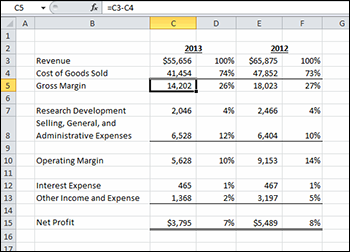
Figure 7-1: A financial statement for a manufacturing company.

How it works

The gross margin formula simply subtracts cell C4 from cell C3. The gross margin percent divides C5 by C3, but note that the C3 reference is absolute because it has dollar signs. Making the reference absolute allows you to copy the formula to other lines on the income statement to see the percentage of revenue, a common analysis performed on income statements.

Alternative: Calculating Markup

Markup is often confused with gross margin percent, but they are different. Markup is the percentage added to costs to arrive at a selling price. Figure 7-2 shows the sale of a single product, the markup applied, and the gross margin realized when sold.

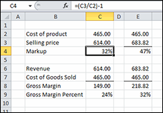
Figure 7-2: Markup and gross margin percent from a single product.

The markup is computed by dividing the selling price by the cost and subtracting 1:

=(C3/C2)-1

By marking up the cost of the product 32 percent, you achieve a 24 percent gross margin. If you want to mark up a product to get a 32 percent margin (as shown in column E of Figure 7-2), use the following formula:

=1/(1-E9)-1

Using this formula, you would need to mark up this product 47 percent if you wanted your income statement to show a 32 percent gross margin.

Formula 68: Calculating EBIT and EBITDA

Earnings before interest and taxes (EBIT) and earnings before interest, taxes, depreciation, and amortization (EBITDA) are common calculations for evaluating the results of a business. Both are computed by adding back certain expenses to earnings, also known as net profit.

Figure 7-3 shows an income statement and the results of the EBIT and EBITDA calculations below it.

EBIT: =C18+VLOOKUP("Interest Expense",$B$2:$C$18,2,FALSE)+VLOOKUP("Income Tax Expense",$B$2:$C$18,2,FALSE)
EBITDA: =C20+VLOOKUP("Depreciation Expense",$B$2:$C$18,2,FALSE)+VLOOKUP("Amortization Expense",$B$2:$C$18,2,FALSE)

How it works

The EBIT formula starts with net loss in C18 and uses two VLOOKUP functions to find Interest Expense and Income Tax Expense from the income statement. For EBITDA, the formula starts with the result of the EBIT calculation and uses the same VLOOKUP technique to add back Depreciation Expense and Amortization Expense.

You benefit from using VLOOKUP rather than simply using the cell references to those expenses. If the lines on the income statement are moved around, the EBIT and EBITDA formulas don’t need to be changed.

See Chapter 6 for more on the VLOOKUP function.

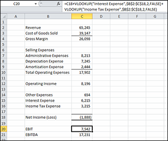
Figure 7-3: An income statement with EBIT and EBITDA calculations.

Formula 69: Calculating Cost of Goods Sold

The term cost of goods sold refers to the amount you paid for all the goods you sold. It is a critical component to calculating gross margin, as demonstrated in Formula 67. If you use a perpetual inventory system, you calculate cost of goods sold for every sale made. For simpler systems, however, you can calculate it based on a physical inventory at the end of the accounting period.

Figure 7-4 shows how to calculate the cost of goods sold with only the beginning and ending inventory counts and the total of all the inventory purchased in the period.

Goods Available for Sale: =SUM(C2:C3)
Cost of Goods Sold: =C4-C5

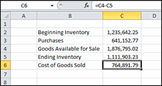
Figure 7-4: Calculating cost of goods sold.

How it works

The goods available for sale is beginning inventory plus all the purchases made. It is an intermediate calculation that shows what your ending inventory would be if you didn’t sell anything.

The cost of goods sold calculation simply subtracts ending inventory from the goods available for sale. If you had the goods at the start of the period or you bought them during the period but you don’t have them at the end of the period, they must have been sold.

Formula 70: Calculating Return on Assets

Return on assets (ROA) is a measure of how efficiently a business is using its assets to generate income. For example, a company with higher ROA can generate the same profit as one with a lower ROA using fewer or cheaper assets.

To compute ROA, divide the profits for a period of time by the average of the beginning and ending total assets. Figure 7-5 shows a simple balance sheet and income statement and the resulting ROA.

=G15/AVERAGE(C12:D12)

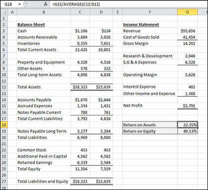
Figure 7-5: A return on assets calculation.

How it works

The numerator is simply the net profit from the income statement. The denominator uses the AVERAGE function to find the average total assets for the period.

Alternative: Calculating return on equity

Another common profitability measure is return on equity (ROE). An investor may use ROE to determine whether her investment in the business is being put to good use. As does ROA, ROE divides net profit by the average of a balance sheet item over the same period. ROE, however, uses average Total Equity rather than average Total Assets. The formula to calculate ROE from Figure 7-5 is as follows:

=G15/AVERAGE(C25:D25)

Formula 71: Calculating Break Even

A business may want to determine how much revenue it will need to achieve a net profit of exactly $0. This revenue result is called break even. To determine it, the business estimates its fixed expenses as well as the percentage of each of its variable expenses. Using those numbers, it can back into a revenue amount that results in break even.

Figure 7-6 shows a break-even calculation. Column C shows either an “F” for a fixed expense or a percentage for an expense that varies as revenue changes. For example, research and development will be spent according to a budget and doesn’t change if revenue increases or decreases. On the other hand, if the business pays a commission, the selling expenses will rise and fall with revenues.

The calculations to determine break even (those numbers where column C is blank) are as follows:

Operating Margin: =SUM(D15:D18)
Margin Net of Variable Expenses: =SUM(D10:D13)
Gross Margin: =SUM(D7:D8)
Revenue: =ROUND(D8/(1-SUM(C4:C7)),0)

The two variable expenses shown in Figure 7-6, Cost of Goods Sold and Selling Expenses, are calculated by multiplying the revenue figure by the percentage. The formulas from Figure 7-6 are as follows:

Cost of Goods Sold: =ROUND(D3*C4,0)
Selling Expenses: =ROUND(D3*C7,0)

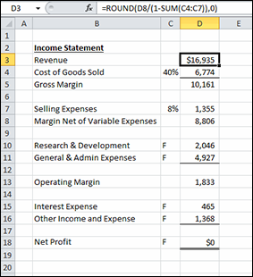
Figure 7-6: A break-even calculation.

How it works

To build the break-even model in Figure 7-6, follow these steps:

1. Enter 0 into cell D18 to indicate zero net profit.
2. Enter the fixed expense amounts in column D next to their labels in column B.
3. Enter the percentage the company pays in commission in cell C7 (8% in this example).
4. Enter a percentage equal to 1 minus the expected gross margin in cell C4. In this example, the company expects a 60 percent gross margin percent, so you enter 40% in C4.
5. In cell D13, enter the formula for Operating Margin shown previously. The Operating Margin must be the sum of Interest Expense and Other Income and Expense. As shown in Figure 7-6, if you estimate Interest Expense to be $465 and Other Income and Expense to be $1,368, Operating Margin must be $1,833 for Net Profit to be zero.
6. In cell D8, enter the formula for Margin Net of Variable Expenses shown previously. This calculation is Operating Margin plus the fixed operating expenses. It will drive the revenue calculation.
7. In cell D7, enter the formula for Selling Expenses shown previously. You haven’t entered the revenue formula yet, so this will be zero for now. After revenue is entered, however, the cell will show the correct value.
8. Enter the formula for Cost of Goods Sold in cell D4. As with the Selling Expenses formula, this formula will return zero until revenue is computed.
9. Finally, enter the formula for Revenue in cell D3. The Revenue calculation divides Margin Net of Variable Expenses by 1 minus the sum of the variable percentages. In Figure 7-6, the two variable expenses will be 48 percent (40 percent plus 8 percent) of revenue. Subtracting 48 percent from 100 percent leaves 52 percent, which is divided into the Margin Net of Variable Expenses to get Revenue.

If this company makes a 60 percent gross margin, pays 8 percent in commissions, and has estimated the fixed expenses accurately, it needs to sell $16,935 to break even.

Formula 72: Calculating Customer Churn

Customer churn is the measure of how many customers you lose in a given period. It’s an important metric to track for subscription-based businesses, although it’s applicable to other revenue models as well. If your growth rate (the rate at which you are adding new customers) is higher than your churn rate, your customer base is growing. If not, you’re losing customers faster than you can add them, and something needs to change.

Figure 7-7 shows a churn calculation for a company with recurring monthly revenue. You need to know the number of customers at the beginning and end of the month and the number of new customers in that month.

Subscribers lost: =C2+C3-C4
Churn rate: =C6/C2

Figure 7-7: Calculating the churn rate.

How it works

To determine the number of customers lost during the month, the number of new customers is added to the number of customers at the beginning of the month. Then the number of customers at the end of the month is subtracted from that total. Finally, the number of customers lost during the month is divided by the number of customers at the beginning of the month to get the churn rate.

In this example, the business has a churn rate of 9.21 percent. It is adding more customers than it is losing, so that churn rate may not be seen as a problem. However, if the churn rate is higher than expectation, the company may want to investigate why it’s losing customers and change its pricing, product features, or some other aspect of its business.

Alternative: Annual churn rate

If a business has monthly recurring revenue, it means that customers sign up and pay for one month at a time. For those companies, it makes sense to calculate the churn rate on a monthly basis. Any new customers during the month will not churn in the same month because they’ve already paid for the month.

A typical magazine, however, signs up subscribers for an annual subscription. A meaningful churn rate calculation for that business would therefore be an annual churn rate. If a business wants to calculate a churn rate for a longer period than its recurring revenue model, such as calculating an annual churn for a business with monthly subscribers, the formula changes slightly. Figure 7-8 shows an annual churn rate calculation.

Annual churn rate: =C6/AVERAGE(C2,C4)

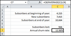
Figure 7-8: Annual churn rate of monthly recurring revenue.

The number of lost subscribers is divided by the average of beginning and ending subscribers. Because the period of the churn rate is different from the period of the recurring revenue, some of those 7,415 new subscribers canceled their subscriptions within the year, albeit in a later month than they first subscribed.

Formula 73: Calculating Average Customer Lifetime Value

Customer Lifetime Value (CLV) is a calculation that estimates the gross margin contributed by one customer over that customer’s life. The churn rate calculated in Formula 72 is a component of CLV.

Figure 7-9 shows a calculation of CLV using the churn rate previously calculated. The first step is to calculate the average gross margin per customer.

Gross margin: =F2-F3
Average customer margin: =F4/AVERAGE(C4,C10)
Customer Lifetime Value: =F6/C7

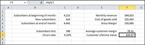
Figure 7-9: Customer Lifetime Value calculation.

How it works

To calculate CLV, follow these steps:

1. Calculate the gross margin as demonstrated in Formula 67: revenue less cost of goods sold.
2. Calculate the average customer margin by dividing the gross margin by the average number of customers for the month. Because the gross margin was earned over the month, you have to divide by the average number of customers instead of either the beginning or ending customer count.
3. Calculate the CLV by dividing the average customer margin by the churn rate.

In this example, each customer will contribute an estimated $828.97 over his or her lifetime.

Formula 74: Calculating Employee Turnover

Employee turnover is a measure of how well an organization is hiring and retaining talent. A high turnover rate indicates that the organization is not hiring the right people or not retaining people, possibly due to inadequate benefits or below-average pay. Separations commonly include both voluntary and involuntary terminations.

Figure 7-10 shows the employment changes of an organization over a 12-month period. New hires are added to and separations are subtracted from the number of employees at the beginning of the month to get the ending employee count.

Average monthly employment: =AVERAGE(F3:F14)
Separations: =SUM(E3:E14)
Employee Turnover: =F17/F16

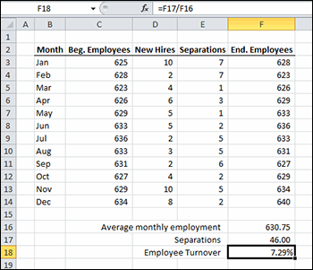
Figure 7-10: Monthly employment changes over one year.

How it works

Employee turnover is simply the ratio of separations to average monthly employment. The AVERAGE function is used to calculate the average ending count of employees over the months. Separations are summed using SUM and are divided by the average monthly employments.

The result can be compared to industry averages or companies in the same industry. Different industries experience different turnover rates, so comparing them can lead to poor decisions. You don’t have to calculate turnover for a 12-month period, but doing so removes seasonal employment variations that can skew results.

Formula 75: Converting Interest Rates

Two common methods for quoting interest rates are the nominal rate and the effective rate:

• Nominal rate: This is the stated rate and is usually paired with a compounding period, for example, 3.75 percent APR compounded monthly. In this example, 3.75 percent is the nominal rate; APR is short for annual percentage rate, meaning the rate is applied on an annual basis; and one month is the compounding period.
• Effective rate: This is the actual rate paid. If the nominal rate period is the same as the compounding period, the nominal and effective rates are identical. However, as is usually the case, when the interest compounds over a shorter period than the nominal rate period, the effective rate will be higher than the nominal rate.

Figure 7-11 shows 12 compounding periods in the middle of a 30-year loan. The original loan was for $165,000, has a nominal rate of 3.75% APR compounded monthly, and calls for 30 annual payments of $9,169.68 each.

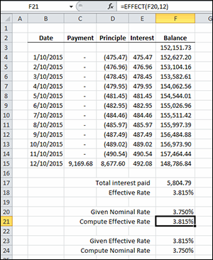
Figure 7-11: A partial amortization schedule to compute the effective rate.

For each period that the interest compounds but no payment is made, the balance goes up by the amount of interest. When the payment is made, a little of it goes to the last month’s interest and the rest of it reduces the principle.

Cell F17 sums all the interest compounded over the year and cell F18 divides it by the beginning balance to get the effective rate. Fortunately, you don’t have to create a whole amortization schedule to convert interest rates. Excel provides the EFFECT and NOMINAL worksheet functions to do that job:

Effective Rate: =EFFECT(F20,12)
Nominal Rate: =NOMINAL(F23,12)

How it works

Both EFFECT and NOMINAL take two arguments: the rate to be converted and the npery argument. The rate to be converted is the effective rate for NOMINAL and the nominal rate for EFFECT. The npery argument is the number of compounding periods in the nominal rate period. In this example, the nominal rate is annual because the term APR was used. A year has 12 months, so your nominal rate has 12 compounding periods. If, for example, you had a loan with an APR that compounded daily, the npery argument would be 365.

Alternative: Computing effective rate with FV

The effective rate can also be computed with the FV function. With such a handy function as EFFECT, you don’t need to resort to FV, but it can be instructive to understand the relationship between EFFECT and FV.

=FV(3.75%/12,12,0,-1)-1

This formula computes the future value of a $1 loan at 3.75 percent compounded monthly for one year and then subtracts the original $1. If you were to take this loan, you would pay back $1.03815 after the year was over. That means you’d owe an additional $0.03815 more than you borrowed, or, effectively, 3.815 percent.

Formula 76: Creating a Loan Payment Calculator

You can use the Excel PMT worksheet function to calculate your monthly payment on a loan. You can hard-code the values, such as the loan amount and interest rate, into the function’s arguments, but by entering those values in cells and using the cells as the arguments, you can easily change the values to see how the payment changes.

Figure 7-12 shows a simple payment calculator. The user enters values in C2:C4 and the payment is calculated in C6 with the following:

=PMT(C3/12,C4*12,C2,0,0)

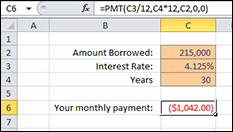
Figure 7-12: A simple loan payment calculator.

How it works

The PMT function takes three required arguments and one optional argument:

• rate (required): The rate argument is the annual nominal interest rate divided by the number of compounding periods in a year. In this example, the interest compounds monthly, so the interest rate in C3 is divided by 12.
• nper (required): The nper argument is the number of payments that will be made over the life of the loan. Because your user input asks for years and the payments are monthly, the number of years in C4 is multiplied by 12.
• pv (required): The pv argument, or present value, is the amount being borrowed. Excel’s loan functions, of which PMT is one, work on a cash flow basis. When you think about present value and payments as cash inflows and outflows, it’s easier to understand when the value should be positive or negative. In this example, the bank is loaning you $215,000, which is a cash inflow and thus positive. The result of the PMT function is a negative because the payments will be cash outflows.

If you want the PMT function to return a positive value, you can change the pv argument to a negative number. That’s like calculating the payment from the bank’s perspective: The loan is a cash outflow and the payments are cash inflows.

The most common mistake in financial formulas is a mismatch between compounding periods and payment frequency. In this example, the rate is divided by 12 to make it a monthly rate and the nper is multiplied by 12 to make it a monthly payment. Both arguments are converted to monthly, so they match and you get the correct result.

If you forgot to divide the rate by 12, Excel would think you were entering a monthly rate, and the payment would be way too high. Similarly, if you entered years for the nper and a monthly rate, Excel would think you were paying only once a year.

Excel doesn’t really know whether you enter months, years, or days. It cares only that the rate and nper match.

Alternative: Creating an amortization schedule

With the payment amount calculated, you can create an amortization schedule that shows how much of each payment is principle and interest and what the loan balance is after each payment. Figure 7-13 shows a portion of the amortization schedule.

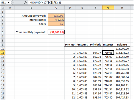
Figure 7-13: A partial amortization schedule.

The columns of the amortization schedule are as follows:

• Pmt No: The number of the payment being made. You enter 1 into D11. Then you enter the formula =D11+1 into D12 and copy it down to D370. (Your amortization schedule can handle 360 payments.)
• Pmt Amt: The amount of the PMT calculation rounded to the nearest penny. Although Excel can calculate a lot of decimal places, you can write a check only for dollars and cents. This means that there will be a small balance at the end of the loan. You enter the formula =-ROUND($C$6,2) into E11 and fill it down through E370.
• Principle: The amount of each payment applied to the loan balance. You enter the formula =E11-G11 into F11 and fill it down through F370.
• Interest: The amount of each payment that is interest. The balance after the prior payment is multiplied by the interest rate divided by 12. The total is rounded to two decimal places. Enter the formula =ROUND(H10*$C$3/12,2) into G11 and fill it down through G370.
• Balance: The balance of the loan after the payment. Enter the formula =C2 in H10 to represent the original amount of the loan. Starting in H11 and continuing down to H370, the formula =H10-F11 reduces the balance by the principle portion of the payment.

In the example shown previously in Figure 7-13, the number of years was entered as 15, compared to 30 in Figure 7-12. Reducing the length of the loan increases the amount of the payment.

The final step is to hide rows beyond the loan term. You accomplish this task with conditional formatting that changes the font color to white. A white font color against a white background effectively hides the data. The formula for the conditional formatting follows and is shown in Figure 7-14.

=$D12>$C$4*12

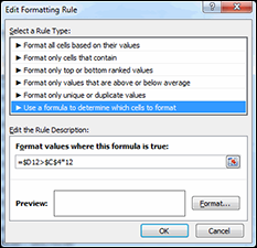
Figure 7-14: Conditional formatting to hide rows.

This formula compares the payment number in column D to the number of years in C4 times 12. When the payment number is larger, the formula returns TRUE and the white font color formatting is applied. When the payment number is less than or equal to the total number of payments, no conditional formatting is applied.

See Chapter 9 for more information on conditional formatting.

Formula 77: Creating a Variable-Rate Mortgage Amortization Schedule

In Formula 76, you create an amortization schedule for a loan with a fixed interest rate. There are also loans for which the rate changes at times during the life of the loan. Often these loans have an interest rate that’s tied to a published index, such as the London Interbank Offered Rate (LIBOR), plus a fixed percentage. Those interest rates are usually stated as “LIBOR plus 3%,” for example.

Figure 7-15 shows an amortization schedule for a loan with a variable interest rate. We added a Rate column to the amortization schedule so that interest rate changes will be obvious. A separate table is used to record when the rate changes.

The Rate column has the following formula to select the proper rate from the rate table:

=VLOOKUP(D11,$K$11:$L$23,2,TRUE)

The Interest column formula changes to use the rate in column G rather than the rate in C3:

=ROUND(I10*G11/12,2)

All other formulas are unchanged from the schedule created in Formula 76.

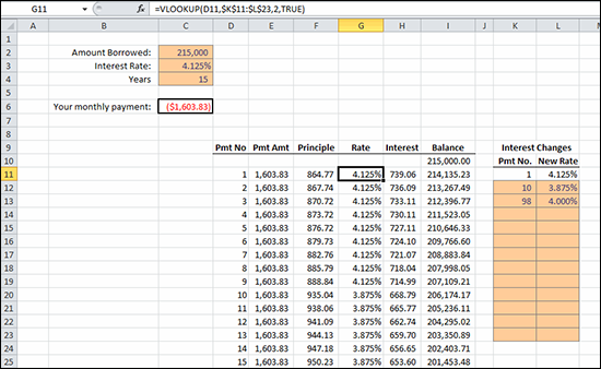
Figure 7-15: A variable-rate amortization schedule.

How it works

The Rate column uses a VLOOKUP with a fourth argument of TRUE. The fourth argument of TRUE requires that the rate table be sorted in ascending order. Then VLOOKUP looks up the payment number in the rate table. It doesn’t require an exact match but returns the row where the next payment number is larger than the lookup value. For instance, when the lookup value is 16, VLOOKUP returns the second row of the rate table because the payment number in the next row, 98, is larger than the lookup value.

See Chapter 6 for more examples of using VLOOKUP.

The interest rate column formula is very similar to the one used in Formula 76 except that the absolute reference to $C$3 is replaced by a reference to column G (G11 for the formula in row 11).

Alternative: Using dates instead of payment numbers

The two amortization schedules for this section and the previous one use the payment number to identify each payment. In reality, those payments are due on the same day of the month. Using a payment number instead of a date, however, allows the amortization schedule to be used for loans that start on any date. Figure 7-16 shows an amortization schedule using dates.

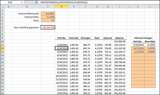
Figure 7-16: A date-based amortization schedule.

To modify the schedule to show the dates, follow these steps:

1. Enter the first payment date in cell D11.
2. Enter the below formula in D12 and fill down.

   =DATE(YEAR(D11),MONTH(D11)+1,DAY(D11))

3. Change the Pmt No column in the rate table (cells K9:L23) to the date the rate changed.
4. Change the formula in the conditional formatting to the following formula:

   =$D12>=DATE(YEAR($D$11),MONTH($D$11)+($C$4*12),DAY($D$11))

Formula 78: Calculating Depreciation

Excel provides a number of depreciation-related worksheet functions including DB, DDB, SLN, and SYD. In this section, you look at calculating straight-line (SLN) and variable-declining balance (VDB) depreciation.

The depreciation for the first and last year of an asset’s life is usually different than for the middle year. A convention is employed so that a full year’s depreciation is not taken for the first year. Common conventions are half-year, mid-month, and mid-quarter. For the half-year convention, the asset is assumed to have been purchased at the halfway point of the year; consequently, one half of a normal year’s depreciation is recorded for that year.

Figure 7-17 shows a depreciation schedule for five assets using the straight-line method and a half-year convention. Columns B:E contain the following user-entered data:

• Asset No.: A unique identifier for each asset. It’s not necessary for the schedule, but is handy for keeping track of assets.
• Cost: The amount paid to put the asset in service. This amount includes the price paid for the asset, any taxes associated with purchase, the cost to ship the asset to its place of service, and any costs to install the asset so that it’s ready for use. This amount is also known as basis or cost basis.
• Year Acquired: The year the asset was put into service. This year may be different from the year the payment was made to purchase the asset. It determines when depreciation starts.
• Useful Life: The number of years you estimate that the asset will provide service.

The formula in F3:N7 is as follows:

=IF(OR(YEAR(F$2)<$D3,YEAR(F$2)>$D3+$E3),0,SLN($C3,0,$E3))*IF(OR(YEAR(F$2)=$D3+$E3,YEAR(F$2)=$D3),0.5,1)

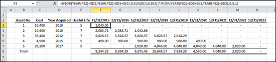
Figure 7-17: A straight-line depreciation schedule.

How it works

The main part of this formula is SLN($C3,0,$E3). The SLN worksheet function computes the straight-line depreciation for one period. It takes three arguments: cost, salvage, and life. For simplicity, the salvage value for this example is set to zero, meaning that the asset’s cost will be fully depreciated at the end of its useful life.

The SLN function is pretty simple. But this is a depreciation schedule, so you have more work to do. The first IF function determines whether the date for that column (in row 2) is within the asset’s useful life. If the year of the date in F2 is less than the year acquired, the asset isn’t in service yet and the depreciation is zero. If F2 is greater than the year acquired plus the useful life, the asset is already fully depreciated, and the depreciation is zero. Both of these conditionals are wrapped in an OR function so that if either is TRUE, the whole expression returns TRUE. If both are FALSE, however, the SLN function is returned.

See Chapter 5 for more examples of using IF with OR.

The second part of the formula is also an IF and OR combination. These conditional statements determine whether the year in F2 is either the first year of depreciation or the last year. If either is TRUE, the straight-line result is multiplied by 0.5, representing the half-year convention employed here.

All the cell references in this formula are anchored so that the formula can be copied down and to the right and so that the cell references change appropriately. References to row 2 are anchored on the row so that you’re always evaluating the date in row 2. References to the columns C:E are anchored on the columns so that Cost, Year Acquired, and Useful Life stay the same as the formula is copied.

See Chapter 1 for more information on relative and absolute cell references.

Alternative: Accelerated depreciation

The straight-line method depreciates an asset equally over all the years of its useful life. Some organizations use an accelerated method, which is a method that depreciates at a higher rate at the beginning of an asset’s life and a lower rate at the end. The theory is that an asset loses more value when it is first put in service than in its last year of operation.

Excel provides the DDB function (double-declining balance) for accelerated depreciation. DDB computes what the straight-line method would be for the remaining asset value and doubles it. The problem with DDB is that it doesn’t depreciate the whole asset within the useful life. The depreciation amount gets smaller and smaller but runs out of useful life before it gets to zero.

The most common application of accelerated depreciation is to start with a declining balance method, and after the depreciation falls below the straight-line amount, the method is switched to straight line for the remaining life of the asset. Fortunately, Excel provides the VDB function, which has that logic built in. Figure 7-18 shows a depreciation schedule using the VDB-based formula as follows:

=IF(OR(YEAR(F$2)<$D3,YEAR(F$2)>$D3+$E3),0,VDB($C3,0,$E3*2,IF(YEAR(F$2)=$D3,0,IF(YEAR(F$2)=$D3+$E3,$E3*2-1,(YEAR(F$2)-$D3)*2-1)),IF(YEAR(F$2)=$D3,1,IF(YEAR(F$2)=$D3+$E3,$E3*2,(YEAR(F$2)-$D3)*2+1))))

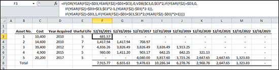
Figure 7-18: An accelerated depreciation schedule.

You might have noticed that this formula is a little more complicated than the SLN formula from the previous example. Don’t worry, we step through it piece by piece for you. Here’s the first part:

=IF(OR(YEAR(F$2)<$D3,YEAR(F$2)>$D3+$E3),0,VDB(...))))

This first part of the formula is identical to the SLN formula described previously in this section. If the date in row 2 is not within the useful life, the depreciation is zero. If it is, the VDB function is evaluated. Following is the VDB function from the IF function’s third argument. There are placeholders for the starting period and ending period arguments of VDB, which we explain later.

VDB($C3,0,$E3*2,starting_period,ending_period)

The first three arguments to VDB are the same as the SLN arguments: cost, salvage value, and life. SLN returns the same value for every period so that you don’t have to tell SLN which period to calculate. But VDB returns a different amount depending on the period. The last two arguments of VDB tell it which period to compute. The life in E3 is doubled, which we explain in the next section.

Starting_period: IF(YEAR(F$2)=$D3,0,IF(YEAR(F$2)=$D3+$E3,$E3*2-1,(YEAR(F$2)-$D3)*2-1))

None of Excel’s depreciation functions takes into account the convention. That is, Excel calculates depreciation as if you bought all your assets on the first day of the year. That’s not very practical. In this section, you assume a half-year convention so that only half of the depreciation is taken in the first and last years. To calculate depreciation on a half-year convention using VDB, you have to trick Excel into thinking that the asset has twice its useful life.

For an asset with a five-year useful life, the period for the first year goes from 0 to 1. For the second year, the periods span 1–3. The third year spans periods 3–5. That pattern continues until the last year, which spans 9–10 (10 is double the five-year life). The starting period portion of the formula evaluates like this:

• If the year to compute is the acquisition year, make the starting period zero.
• If the year to compute is the last year, make the starting period the useful life times two and subtract one.
• For all other years, subtract the acquisition year from the year to compute, multiply by two, and subtract 1.

The ending period portion of the formula is similar to the starting period portion. For the first year, the ending period argument is set to 1. For the last year, it ends at the useful life times 2 minus 1. For the middle years, it does the same calculation except that it adds 1 instead of subtracting.

By doubling the useful life, say from 7 periods to 14 periods for a seven-year asset, you can introduce the half-year convention into a declining balance function like VDB.

Formula 79: Calculating Present Value

The time value of money (TVM) is an important concept in accounting and finance. The idea is that a dollar today is worth less than the same dollar tomorrow. The difference in the two values is the income you can create with that dollar. The income may be interest from a savings account or the return on an investment.

Excel provides several functions for dealing with TVM, such as the PV function for calculating the present value. In its simplest form, PV discounts a future value amount by a discount rate to arrive at the present value. If I promise to pay you $10,000 one year from now, how much would you take today instead of waiting? The following formula and Figure 7-19 show how you would calculate that amount:

=PV(C4,C3,0,-C2)

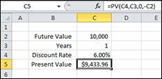
Figure 7-19: A present value calculation.

How it works

The present value calculator in Figure 7-19 suggests that you would take $9,434 now instead of $10,000 a year from now. If you took the $9,434 and were able to earn 6 percent over the next year, you would have $10,000 at the end of the year.

The PV function accepts five arguments:

• rate: Also known as the discount rate, the rate argument is the return you think you could make on your money over the discount period. It is the biggest factor in determining the present value and can also be the hardest to determine. If you’re conservative, you might pick a lower rate — something you’re sure you can achieve. If you were to use the money to pay off a loan with a fixed rate, the discount rate would be easy to determine.
• nper: The nper is the period of time to discount the future value. In this example, the nper is 1 year and is entered in cell C3. The rate and the period must be in the same units. That is, if you enter an annual rate, nper must be expressed as years. If you use a monthly rate, nper must be expressed as months.
• pmt: The pmt argument is the regular payments received over the discount period. When there is only one payment, as in this example, that amount is the future value and the payment amount is zero. The pmt must also the match the nper argument. If your nper is 10 and you enter any nonzero pmt, PV assumes that you’ll get that payment amount 10 times over the discount period. The next example shows a present value calculation with payments.
• fv: The future value amount is the amount you will receive at the end of the discount period. Excel’s financial function works on a cash flow basis. That means the future value and present value have opposite signs. For this example, the future value was made negative so the formula result would return a positive number.
• type: The type argument can be 0 if the payments are received at the end of the period or 1 if the payments are received at the beginning of the period. The type argument has no effect on this example because the payment amount is zero. The type argument can be omitted, in which case it is assumed to be 0.

Alternative: Calculating the present value of future payments

Another use of PV is to calculate the present value of a series of equal future payments. If, for example, you owe $5,000 of rent for an office over the next 10 years, you can use PV to calculate how much you would be willing to pay to get out of the lease. Figure 7-20 shows the present-value calculation for that scenario.

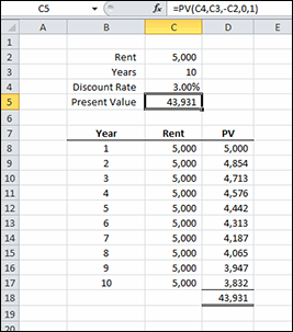
Figure 7-20: The present value of a series of future payments.

Here’s the PV formula used in Figure 7-20:

=PV(C4,C3,-C2,0,1)

If your landlord thought he could make 3 percent on the money, he may be willing to accept $43,930 instead of ten $5,000 payments over the next 10 years. The type argument is set to 1 in this example because rents are usually paid at the beginning of the period.

When used on payments, the PV function actually takes the present value of each payment individually and adds up all the results. Figure 7-20 shows the calculation broken out by payment. The first payment’s present value is the same as the payment amount because it’s due now. The Year 2 payment is due one year from now and is discounted to $4,854. The last payment, due nine years from now, is discounted to $3,832. All the present value calculations are added up. Fortunately, PV does all the heavy lifting for you.

Formula 80: Calculating Net Present Value

The PV function from Formula 79 can calculate the present value of future cash flows if all the cash flows are the same. But sometimes that’s not the case. The NPV (net present value) function is the Excel solution to calculating the present value of uneven future cash flows.

Suppose that someone wanted you to invest $30,000 in a new business. In exchange for your investment, you would be entitled to an annual dividend over the next seven years. The estimated amounts of those dividends are shown in the schedule in Figure 7-21. Further suppose that you would like to earn an 8 percent return on your money.

To determine whether this investment is worth your while, you can use the following NPV function to calculate the net present value of that investment:

=NPV(C2,C5:C11)

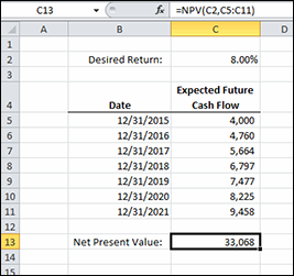
Figure 7-21: The net present value of expected future cash flows.

How it works

NPV discounts each cash flow separately based on the rate, just as PV value does. Unlike PV, however, NPV accepts a range of future cash flows rather than just a single payment amount. NPV doesn’t have an nper argument because the number of values in the range determines the number of future cash flows.

Although the payments can be for different amounts, they are still assumed to be at regular intervals (one year, in this example). Also, as with the other TVM functions in this chapter, the rate period must be consistent with the payment period. In this example, the 8 percent return you’d like is an annual return and the payments are annual, so they match. If you were getting a quarterly dividend, you would have to adjust the rate to a quarterly return.

The NPV for these cash flows calculates to $33,068. Because the required investment to get those cash flows, $30,000, is less than the NPV (and assuming that the estimates are correct), these would be good investments. In fact, this data shows that you would make something more than the 8 percent return you wanted.

Alternative: Positive and negative cash flows

In the previous example, you were asked to make a large, up-front investment to get future cash flows. Another scenario in which you can use NPV is when you make smaller payments at the beginning of the investment period with the expectation of future cash inflows at the end.

Instead of one $30,000 payment, assume that you would only have to invest $15,000 the first year, $10,000 the second year, and $5,000 the third year. The amount you’re required to invest goes down as the business grows and is able to use its own profits to grow. By year four, no more investment is required and the business is expected to be profitable enough to start paying a dividend.

Figure 7-22 shows a schedule that you pay in to for the first three years and get money back the last four. The NPV function is the same as before; just the inputs have changed.

=NPV(C2,C5:C11)

In the first NPV example, the amount invested was not part of the calculation. You simply took the result of the NPV function and compared it to the investment amount. In this example, a portion of the investment is also in the future, so the invested amounts are shown as negatives (cash outflows) and the eventual dividends are shown as positive amounts (cash inflows).

Instead of comparing the result to an initial investment amount, this NPV calculation is compared to zero. If the NPV is greater than zero, the series of cash flows returns something greater than 8 percent. If it’s less than zero, the return is less than 8 percent. Based on the data in Figure 7-22, it’s a good investment.

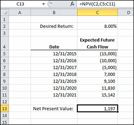
Figure 7-22: The net present value of both positive and negative cash flows.

Formula 81: Calculating an Internal Rate of Return

In Formula 80, you calculate the net present value of future expected cash flows and compare it to the initial investment amount. Because the net present value was greater than the initial investment, you knew the rate of return would be greater than the desired rate. But what is the actual rate of return?

You can use the Excel IRR function to calculate the internal rate of return of future cash flows. IRR is very closely related to NPV. IRR computes the rate of return that causes the NP of those same cash flows to be exactly zero.

For IRR, you have to structure the data a little differently. You have to have at least one positive and one negative cash flow in the values range. If you have all positive values, that means you invest nothing and only receive money. That would be a great investment, but it’s not very realistic. Typically, the cash outflows are at the beginning of the investment period and the cash inflows are at the end. But it’s not always that way, as long as there is at least one inflow and one outflow.

Figure 7-23 shows the same dividend schedule as Formula 80, but you have to include the initial investment for IRR to work. You add the first row to show the initial $30,000 investment. The following IRR formula shows that the investment return is 10.53 percent.

=IRR(C3:C10,0.08)

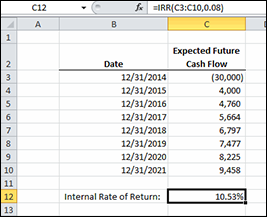
Figure 7-23: The internal rate of return of a series of future cash flows.

How it works

The first argument for IRR is the range of cash flows. The second argument is a guess of what the internal rate of return will be. If you don’t supply a guess, Excel uses 10 percent as the guess argument. IRR works by calculating the present value of each cash flow based on the guessed rate. If the sum of those present value calculations is greater than zero, it reduces the rate and tries again. Excel keeps iterating through rates and summing present values until the sum is zero. When the present values sum to zero, it returns that rate.

Alternative: Nonperiodic future cash flows

For both the NPV function in Formula 80 and the IRR function shown previously, the future cash flows are assumed to be at regular intervals. That may not always be the case, though. For cash flows at irregular intervals, Excel provides the XIRR function.

XIRR requires one more argument than IRR does: dates. IRR doesn’t need to know the dates because it assumes that the cash flows are the same distance apart. Whether they are one day or one year apart, IRR doesn’t care. The rate it returns will be consistent with the cash flows. That is, if the cash flows are annual, the rate will be an annual rate. If the cash flows are quarterly, the rate will be quarterly.

XIRR has a related function for calculating the net present value of nonperiodic cash flows called XNPV. As does XIRR, XNPV requires a matching range of dates.

Figure 7-24 shows a schedule of nonperiodic cash flows. On some days, the investment loses money and requires a cash injection. On other days, the investment makes money and returns it to the investor. Over all the cash flows, the investor makes an annual return of 10.14 percent. The following formula uses XIRR to calculate the return:

=XIRR(C3:C17,B3:B17,0.08)

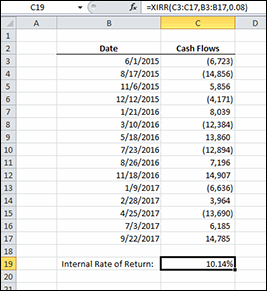
Figure 7-24: The internal rate of return of nonperiodic cash flows.

Internally, XIRR works much the same as IRR. It calculates the present value of each cash flow individually, iterating through rates until the sum of the present values is zero. It bases the present-value calculations on the number of days between the current cash flow and the one just previous in date order. Then it annualizes the rate of return.