page 474
CHAPTER
THIRTEEN
13
Progress and Performance Measurement and Evaluation
page 475
How does a project get one year late?
. . . One day at a time.
—Frederick P. Brooks, The Mythical Man Month, p. 153
Nothing ever goes completely according to plan. Once a project is launched, management needs an information and control system to make adjustments and steer the project toward its objectives. On time-sensitive projects, project managers need to be able to track progress and know when to speed things up. On set budget projects, project managers need to be able to monitor costs and know when it is necessary to cut costs. Not only are you interested in whether the project is on schedule and budget, but management and customers want to know when the project is likely to be completed and at what cost.
This chapter begins by describing the structure and process of project control systems. Indicators used to assess meeting schedule are discussed next, followed by an introduction to Earned Value Management (EVM). Earned value is a key concept. It will be used both to assess current performance and to predict final costs and completion dates. Be forewarned this is not an easy chapter. Measuring progress can seem complicated quickly and you may find yourself overwhelmed by terminology and indices. However, if you master these concepts, you will have a distinct advantage.
page 476
13.1 Structure of a Project Monitoring Information System
A project monitoring system involves determining what data to collect; how, when, and who will collect the data; analysis of the data; and reporting current progress.
What Data Are Collected?
Data collected are determined by which metrics will be used for project control. Typical key data collected are actual activity duration times, resource usage and rates, and actual costs, which are compared against planned times, resources, and budgets. Since a major portion of the monitoring system focuses on cost/schedule concerns, it is crucial to provide the project manager and stakeholders with data to answer questions such as
What is the current status of the project in terms of schedule and cost?
How much will it cost to complete the project?
When will the project be completed?
Are there potential problems that need to be addressed now?
What, who, and where are the causes for cost or schedule overruns?
If there is a cost overrun midway in the project, can we forecast the overrun at completion?
The performance metrics you need to collect should support answering these questions. Examples of specific metrics and tools for collecting data will be discussed in detail later in this chapter.
Collecting Data and Analysis
With the determination of what data are collected, the next step is to establish who, when, and how the data will be assembled. Will the data be collected by the project team, contractor, independent cost engineers, project manager? Or will the data be derived electronically from some form of surrogate data such as cash flow, machine hours, labor hours, or materials in place? Should the reporting period be one hour, one day, one week, or what? Is there a central repository for the data collected and is someone responsible for its dissemination?
Electronic means of collecting data have vastly improved data assembly, analysis, and dissemination. Numerous software vendors have programs and tools to analyze customized collected data and present it in a form that facilitates monitoring the project, identifying sources of problems, and updating the plan.
Reports and Reporting
First, who gets the progress reports? We have already suggested that different stakeholders and levels of management need different kinds of project information. Senior management’s major interests are usually “Are we on time and within budget? If not, what corrective action is taking place?” Likewise, an IT manager working on the project is concerned primarily about her deliverable and specific work packages. The reports should be designed for the right audience.
Typically project progress reports are designed and communicated in written or oral form. A common topic format for progress reports follows:
Progress since last report
Current status of project
page 477Schedule
Cost
Scope
Cumulative trends
Problems and issues since last report
Actions and resolution of earlier problems
New variances and problems identified
Corrective action planned
Given the structure of your information system and the nature of its outputs, you can use the system to interface and facilitate the project control process. These interfaces need to be relevant and seamless if control is to be effective.
13.2 The Project Control Process
Control is the process of comparing actual performance against plan to identify deviations, evaluate possible alternative courses of actions, and take appropriate corrective action. The project control steps for measuring and evaluating project performance are
Setting a baseline plan.
Measuring progress and performance.
Comparing plan against actual.
Taking action.
Each of the control steps is described in the following paragraphs.
Step 1: Setting a Baseline Plan
The baseline plan provides the elements for measuring performance. The baseline is derived from the cost and duration information found in the work breakdown structure (WBS) database and time-sequence data from the network and resource scheduling decisions. From the WBS the project resource schedule is used to time-phase all work, resources, and budgets into a baseline plan. See Chapter 8.
Step 2: Measuring Progress and Performance
Time and budgets are quantitative measures of performance that readily fit into the integrated information system. Qualitative measures such as meeting customer technical specifications and product function are most frequently determined by on-site inspection or actual use. This chapter is limited to quantitative measures of time and budget. Measurement of time performance is relatively easy and obvious. That is, is the critical path early, on schedule, or late; is the slack of near-critical paths decreasing to cause new critical activities? Measuring performance against budget (e.g., money, units in place, labor hours) is more difficult and is not simply a case of comparing actual versus budget. Earned value is necessary to provide a realistic estimate of performance against a time-phased budget. Earned value (EV) is the budgeted cost of the work performed.
Step 3: Comparing Plan against Actual
Because plans seldom materialize as expected, it becomes imperative to measure deviations from plan to determine if action is necessary. Periodic monitoring and page 478measuring the status of the project allow for comparisons of actual versus expected plans. It is crucial that the timing of status reports be frequent enough to allow for early detection of variations from plan and early correction of causes. Usually status reports should take place every one to four weeks to be useful and allow for proactive correction.
Step 4: Taking Action
If deviations from plans are significant, corrective action will be needed to bring the project back in line with the original or revised plan. For example, if the project is behind schedule, overtime may be authorized to get back on schedule. In some cases, conditions or scope can change, which in turn will require a change in the baseline plan to recognize new information.
The remainder of this chapter describes and illustrates monitoring systems, tools, and components to support managing and controlling projects. Several of the tools you developed in the planning and scheduling chapters now serve as input to your information system for monitoring performance. Monitoring time performance is discussed first, followed by cost performance.
13.3 Monitoring Time Performance
A major goal of progress reporting is to catch any negative variances from plan as early as possible to determine if corrective action is necessary. Fortunately, monitoring schedule performance is relatively easy. The project network schedule, derived from the WBS/OBS, serves as the baseline to compare against actual performance.
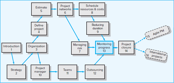
Gantt charts (bar charts), control charts, and milestone schedules are the typical tools used for communicating project schedule status. As suggested in Chapter 6, the Gantt chart is the most favored, used, and understandable. This kind of chart is commonly referred to as a tracking Gantt chart. Adding actual and revised time estimates to the Gantt chart gives a quick overview of project status on the report date.
Tracking Gantt Chart
Figure 13.1 presents a baseline Gantt chart and a tracking Gantt chart for a project at the end of period 6. The solid bar below the original schedule bar represents the actual start and finish times for completed activities or any portion of an activity completed (see activities A, B, C, D, and E). For example, the actual start time for activity C is period 2; the actual finish time is period 5; the actual duration is three time units, rather than four scheduled time periods. Activities in process show the actual start time; the extended bar represents the expected remaining duration (see activities D and E). The remaining duration for activities D and E are shown with the hatched bar. Activity F, which has not started, shows a revised estimated actual start (9) and finish time (13).
FIGURE 13.1
Baseline and Tracking Gantt Charts
Note how activities can have durations that differ from the original schedule, as in activities C, D, and E. Either the activity is complete and the actual is known, or new information suggests the estimate of time be revised and reflected in the status report. Activity D’s revised duration results in an expected delay in the start of activity F. The project is now estimated to be completed one period later than planned. Although sometimes the Gantt chart does not show dependencies, when it is used with a network, the dependencies are easily identified if tracing is needed.
page 479
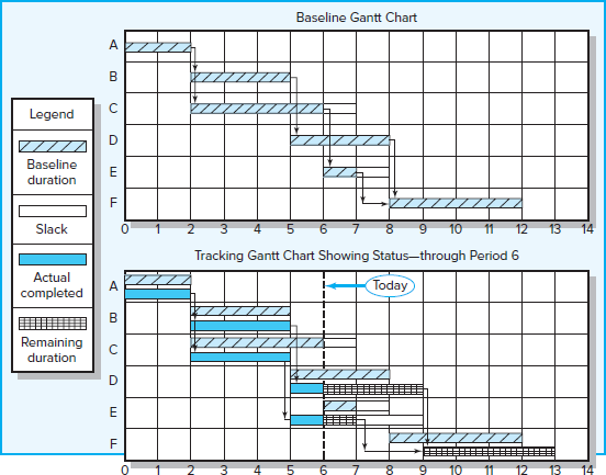
Control Chart
A control chart is another tool used to monitor past project schedule performance and current performance and to estimate future schedule trends. Figure 13.2 depicts a project control chart. The chart is used to plot the difference between the scheduled and actual times on the critical path at a given point on the project. Although Figure 13.2 shows the project was behind early in the project, the plot suggests corrective action brought the project back on track. If the trend is sustained, the project will come in ahead of schedule. Because the activity scheduled times represent average durations, four observations trending in one direction indicate there is a very high probability that there is an identifiable cause. The cause should be located and action taken if necessary. Control chart trends are very useful for warning of potential problems so appropriate action can be taken if necessary.
FIGURE 13.2
Project Schedule Control Chart
Milestone Schedules
Milestone schedules are often used to keep more distal stakeholders informed on the progress of a project. Such stakeholders, whether it is senior management, the owner, or regulatory agencies, often neither need nor desire a detailed accounting of project progress. Instead, their interests can be satisfied by reporting progress toward major project milestones. Remember from Chapter 4 that milestones are significant project events that mark major accomplishments. Following is the milestone schedule used to keep the president of a university and his cabinet informed on the construction of a new College of Business building.
page 480
| Completion Dates: | |
|
|
Project managers recognize the need to use a more macro schedule of significant deliverables to keep external stakeholders informed and a more detailed milestone-driven schedule to manage and motivate the project team to achieve those deliverables. For more on the latter, see Snapshot from Practice 13.1: Guidelines for Setting Milestones.
13.4 Earned Value Management (EVM)
The Need for Earned Value Management
Earned value management (EVM) is a methodology that combines scope, schedule, and resource measurements to assess project performance and progress. To understand the value of EVM, imagine you are a project manager for a large painting company that has secured the contract with a local developer to paint 10 identical condos. It is estimated that it will take your team 2 weeks to paint each condo at a cost of $10,000. You expect to complete the project in 20 weeks at a total cost of $100,000.
page 481
After 10 weeks management asks for a status report. You report you have spent $50,000. Management might conclude the following: good, you spent as much as you were supposed to spend, and everything is going according to plan. This might be correct, but it might not be. It is also possible that after 10 weeks due to unusually warm weather you were able to paint 6 condos at a cost of only $50,000. Conversely, due to inclement weather you may have been able to paint only 4 condos at a cost of $50,000. What is true?
From this example it is easy to understand why using only actual and planned costs can mislead management and customers in evaluating project performance. Cost variance of budget-to-actual alone is inadequate. It does not measure how much work was accomplished for the money spent.
Enter the concept of earned value (EV). Earned value is the budgeted cost of the work you have actually accomplished to date. Let’s return to the previous examples and include EV in the analysis.
Management thank you for cost information but want to know how much work has been accomplished. You survey the work site and report that 4½ condos have been page 482painted. According to the budget, 4½ condos should have cost $4,500. You earn the value of the work that has been completed.
Earned value for the first ten weeks is $45,000.
Actual costs for the first ten weeks are $50,000.
Planned budget costs for the first ten weeks are $50,000.
We can now infer with confidence that the project is (1) behind schedule—we have accomplished $5,000 (one-half a condo) less than planned and (2) overbudget—we spent $50,000 to accomplish $45,000 worth of work.
Now let’s assume you survey the site and instead of finding 4½ condos painted, you are happy to report that 6 have been painted. You earn the value of the work that has been accomplished (6 × $10,000) = $60,000. Now you can report that the project is both (1) ahead of schedule—we have accomplished $10,000 (one condo) worth of work more than planned and (2) underbudget—we were able to paint 6 condos for only $50,000 instead of the estimated $60,000.
Earned value is not new. The original earned value cost/schedule system was pioneered by the U.S. Department of Defense (DoD) in the 1960s. Cost overruns and public outcry motivated the DoD to search for a more effective system to track schedule and cost in large project contracts. The private sector was quick to recognize the worth of EVM. It is probably safe to say project managers in every major country are using some form of EVM. It is not limited to construction or contracts. EVM is being used on internal projects in the manufacturing, pharmaceutical, and high-tech industries. For example, organizations such as EDS, NCR, Levi Strauss, Tektronics, and Disney have used earned value systems to track projects. More recently one of the authors used his expertise in EVM to help the College of Oceanography (CoO) at Oregon State University secure a multimillion-dollar National Science Foundation (NSF) grant to design and build the next generation of off-shore research vessels. This was the first time CoO encountered an NSF grant application that required an EVM system.
The earned value system starts with the time-phased costs that provide the project budget baseline, which is called the planned budgeted value of the work scheduled (PV). Given this time-phased baseline, comparisons can be made with actual and planned schedule and costs using a concept called earned value. The earned value system uses data developed from the work breakdown structure, project network, and schedule. This integrated cost/schedule system provides schedule and cost variance and can be used to forecast the remaining costs for the in-process project. The earned value approach provides the missing links not found in conventional cost-budget systems. At any point in time, a status report can be developed for the project. The development of an integrated cost/schedule system is discussed next.
EVM uses several acronyms and equations for analysis. Table 13.1 presents a glossary of these acronyms. You will need this glossary as a reference. In recent years acronyms have been shortened to be more phonetically friendly. This movement is reflected in material from the Project Management Institute, in project management software, and by most practitioners. This text edition follows the recent trend. The acronyms found in brackets represent the older acronyms, which are often found in software programs. To the uninitiated, the terms used in practice appear horrendous and intimidating. However, once a few basic terms are understood, the intimidation index will evaporate.
TABLE 13.1
Glossary of Terms
| EV | Earned value for a task is the budgeted value of the work accomplished. Work accomplished is often measured in terms of percentages (e.g., 25% complete) in which case, EV is simply percent complete times its original budget. [The older acronym for this value was BCWP—budgeted cost of the work performed.] |
| PV | The planned time-phased baseline of the value of the work scheduled. An approved cost estimate of the resources scheduled in a time-phased cumulative baseline [BCWS—budgeted cost of the work scheduled]. |
| AC | Actual cost of the work completed. The sum of the costs incurred in accomplishing work [ACWP—actual cost of the work performed]. |
| CV | Cost variance is the difference between the earned value and the actual costs for the work completed to date where CV = EV − AC. |
| SV | Schedule variance is the difference between the earned value and the baseline to date where SV = EV − PV. |
| BAC | Budgeted cost at completion. The total budgeted cost of the baseline or project cost accounts. |
| EAC | Estimated cost at completion |
| ETC | Estimated cost to complete remaining work |
| VAC | Cost variance at completion. VAC indicates expected actual over- or underrun cost at completion. |
Carefully following five steps ensures that the cost/schedule system is integrated. These steps are outlined here. Steps 1, 2, and 3 are accomplished in the planning stage. Steps 4 and 5 are sequentially accomplished during the execution stage of the project.
page 483
Define the work using a WBS. This step involves developing documents that include the following information (see Chapters 4 and 5):
Scope.
Work packages.
Deliverables.
Organization units.
Resources.
Budgets for each work package.
Develop work and resource schedule.
Schedule resources to activities (see Chapter 8).
Time-phase work packages into a network.
Develop a time-phase budget using work packages included in an activity. The cumulative values of these budgets will become the baseline and will be called the planned budgeted cost of the work scheduled (PV). The sum should equal the budgeted amounts for all the work packages in the cost accounts (see Chapter 8).
At the work package level, collect the actual costs for the work performed. These costs will be called the actual cost of the work completed (AC). Collect percent complete and multiply this times the original budget amount for the value of the work actually completed. These values will be called earned value (EV).
Compute the schedule variance (SV) (SV = EV − PV) and cost variance (CV) (CV = EV − AC). Prepare hierarchical status reports for each level of management—from work package manager to customer or project manager. The reports should also include project rollups by organization unit and deliverables. In addition, actual time performance should be checked against the project network schedule.
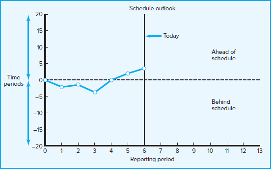
Figure 13.3 presents a schematic overview of the integrated information system, which includes the techniques and systems presented in earlier chapters. Those who have tenaciously labored through the early chapters can smile! Steps 1 and 2 are already carefully developed. Observe that control data can be traced backward to specific deliverables and organization unit responsible.
page 484
FIGURE 13.3
Project Management Information System Overview
The major reasons for creating a baseline are to monitor and report progress and to estimate cash flow. Therefore, it is crucial to integrate the baseline with the performance measurement system. Costs are placed (time-phased) in the baseline exactly as managers expect them to be “earned.” This approach facilitates tracking costs to their point of origin. In practice, the integration is accomplished by using the same rules in assigning costs to the baseline as those used to measure progress using earned value. You may find several rules in practice, but percent complete is the workhorse most commonly used. Someone familiar with each task estimates what percent of the task has been completed or how much of the task remains.
Percent Complete Rule
This rule is the heart of any earned value system. The best method for assigning costs to the baseline under this rule is to establish frequent checkpoints over the duration of the work package and assign completion percentages in dollar terms. For example, units completed could be used to assign baseline costs and later to measure progress. Units might be lines of code, hours, drawings completed, cubic yards of concrete in place, workdays, prototypes complete, and so on. This approach to percent complete adds “objectivity” to the subjective observation approaches often used. When measuring percent complete in the monitoring phase of the project, it is common to limit the amount earned to 80 or 90 percent until the work package is 100 percent complete.
What Costs Are Included in Baselines?
The baseline (PV) is the sum of the cost accounts, and each cost account is the sum of the work packages in the cost account. Three direct costs are typically included in baselines—labor, equipment, and materials—because these are direct costs the project manager can control. Overhead costs and profit are typically added later by page 485accounting processes. Most work packages should be discrete and of short time span and have measurable outputs. If materials and equipment are a significant portion of the cost of work packages, they can be budgeted in separate work packages and cost accounts.
Methods of Variance Analysis
Generally the method for measuring accomplishments centers on two key computations:
Comparing earned value with the expected schedule value.
Comparing earned value with the actual costs.
These comparisons can be made at the project level or down to the cost account level. Project status can be determined for the latest period, all periods to date, and estimated to the end of the project.
Assessing the current status of a project using the earned value cost/schedule system requires three data elements—planned cost of the work scheduled (PV), budgeted cost of the work completed (EV), and actual cost of the work completed (AC). From these data the schedule variance (SV) and cost variance (CV) are computed each reporting period. A positive variance indicates a desirable condition, while a negative variance suggests problems or changes that have taken place.
Cost variance tells us if the work accomplished costs more or less than was planned at any point over the life of the project. If labor and materials have not been separated, cost variance should be reviewed carefully to isolate the cause to either labor or materials—or to both.
Schedule variance presents an overall assessment of all work packages in the project scheduled to date. It is important to note schedule variance contains no critical path information. Critical and noncritical activities are combined in the calculation. Schedule variance measures progress in dollars rather than time units. Therefore, it is unlikely that any translation of dollars to time will yield accurate information telling if any milestone or critical path is early, on time, or late (even if the project occurs exactly as planned). The only accurate method for determining the true time progress of the project is to compare the project network schedule against the actual network schedule to measure if the project is on time (refer to Figure 13.1). However, SV is very useful in assessing the direction all the work in the project is taking—after 20 or more percent of the project has been completed.
Figure 13.4 presents a sample cost/schedule graph with variances identified for a project at the current status report date. Note the graph also focuses on what remains to be accomplished and any favorable or unfavorable trends. The “today” label marks the report date (time period 25) of where the project has been and where it is going. Because our system is hierarchical, graphs of the same form can be developed for different levels of management. In Figure 13.4 the top line represents the actual costs (AC) incurred for the project work to date. The middle line is the baseline (PV) and ends at the scheduled project duration (45). The bottom line is the budgeted value of the work actually completed to date (EV), or the earned value. The dotted line extending the actual costs from the report date to the new estimated completion date represents revised estimates of expected actual costs; that is, additional information suggests the costs at completion of the project will differ from what was planned. Note that the project duration has been extended and the variance at completion (VAC) is negative (BAC − EAC).
FIGURE 13.4
Cost/Schedule Graph
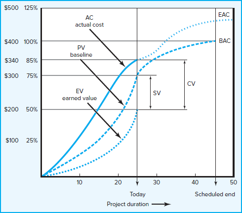
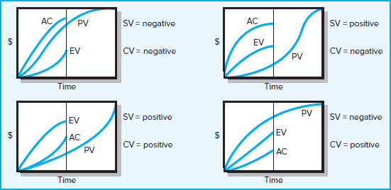
Another interpretation of the graph uses percentages. At the end of period 25, 75 percent of the work was scheduled to be accomplished. At the end of period 25, page 486the value of the work accomplished is 50 percent. The actual cost of the work completed to date is $340, or 85 percent of the total project budget. The graph suggests the project will have about an 18 percent cost overrun and be five time units late. The current status of the project shows the cost variance (CV) to be over budget by $140 (EV − AC = 200 − 340 = −140). The schedule variance (SV) is negative $100 (EV − PV = 200 − 300 = −100), which suggests the project is behind schedule. Before moving to an example, consult Figure 13.5 to practice interpreting the outcomes of cost/schedule graphs. Remember, PV is your baseline and anchor point.
FIGURE 13.5
Earned Value Review Exercise
page 487
13.5 Developing a Status Report: A Hypothetical Example
Working through an example demonstrates how the baseline serves as the anchor from which the project can be monitored using earned value techniques.
Assumptions
Because the process becomes geometrically complex with the addition of project detail, some simplifying assumptions are made in the example to more easily demonstrate the process:
Assume each cost account has only one work package, and each cost account will be represented as an activity on the network.
The project network early start times will serve as the basis for assigning the baseline values.
From the moment work on an activity task begins, some actual costs will be incurred each period until the activity is completed.
Baseline Development
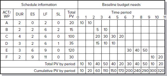
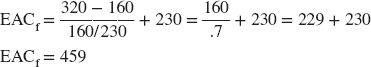
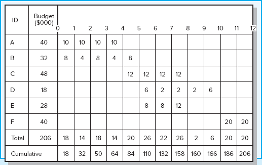
Figure 13.6 (Work Breakdown Structure with Cost Accounts) depicts a simple work breakdown structure (WBS/OBS) for a project with the objective of developing a new digital camera. There are six deliverables (Design Specifications, Shell & Power, Memory/Software, Zoom System, Assemble, and Test), and five responsible departments (Design, Shell, Storage, Zoom, and Assembly). The total for all the cost accounts (CA) page 488is $320,000, which represents the total project cost. Figure 13.7, derived from the WBS, presents a planning Gantt chart for the Digital Camera project. The planned project duration is 11 time units. This project information is used to time-phase the project budget baseline. Figure 13.8 (project baseline budget) presents a worksheet with an early start baseline developed with costs assigned. They are assigned “exactly” as managers plan to monitor and measure schedule and cost performance.
FIGURE 13.6 Work Breakdown Structure with Cost Accounts
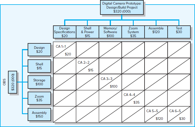
FIGURE 13.7
Digital Camera Prototype Project Baseline Gantt Chart
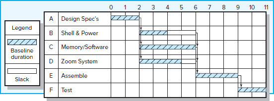
FIGURE 13.8
Digital Camera Prototype Project Baseline Budget ($000)
Development of the Status Report
A status report is analogous to a camera snapshot of a project at a specific point in time. The status report uses earned value to measure schedule and cost performance. Measuring earned value begins at the work package level. Work packages are in one of three conditions on a report date:
Not yet started.
Finished.
In process or partially complete.
Earned values for the first two conditions present no difficulties. Work packages that are not yet started earn zero percent of the PV (budget). Packages that are completed earn 100 percent of their PV. In-process packages apply the percent complete rule to the PV baseline to measure earned value (EV). In our camera example we will only use the percent complete rule to measure progress.
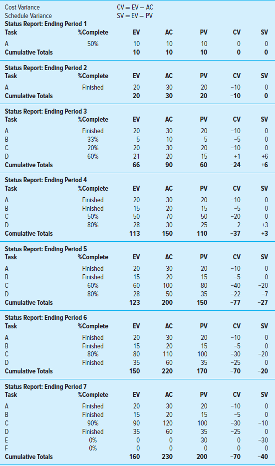
Table 13.2 presents the completed, separate status reports of the Digital Camera Prototype project for periods 1 through 7. Each period percent complete and actual page 489cost were gathered for each task from staff in the field. The schedule and cost variance are computed for each task and the project to date. For example, the status in period 1 shows only Task A (Design Specifications) is in process and it is 50 percent complete and actual cost for the task is 10. The planned value at the end of period 1 for Task A is 10 (see Figure 13.8). The cost and schedule variance are both zero, which indicates the project is on budget and schedule. By the end of period 3, Task A is finished. Task B (Shell & Power) is 33 percent complete and AC is 10; Task C is 20 percent complete and AC is 30; and Task D is 60 percent complete and AC is 20. Again, from Figure 13.8 at the end of period 3, we can see that the PV for Task A is 20 (10 + 10 = 20), for Task B is 5, for Task C is 20, and for Task D is 15. At the end of period 3 it is becoming clear the actual cost (AC) is exceeding the value of the work completed (EV). The cost variance (see Table 13.2) for the project at the end of period 3 is negative 24. Schedule variance is positive 6, which suggests the project may be ahead of schedule.
TABLE 13.2
Digital Camera Prototype Status Reports: Periods 1–7
page 490
It is important to note that since earned values are computed from costs (or sometimes labor hours or other metrics), the relationship of costs to time is not one-for-one. For example, it is possible to have a negative SV variance when the project is actually ahead on the critical path. This occurs when delays in noncritical activities outweigh progress on the critical path. Therefore, it is important to remember that SV is in dollars and is not an accurate measure of time; however, it is a fairly good indicator of the status of the whole project in terms of being ahead or behind schedule after the project is over 20 percent complete. Only the project network, or tracking Gantt chart, and actual work completed can give an accurate assessment of schedule performance down to the work package level.
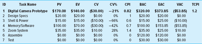
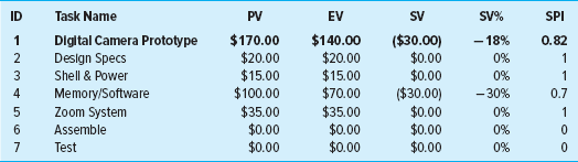
By studying the separate status reports for periods 5 through 7, you can see the project will be over budget and behind schedule. By period 7, Tasks A, B, and D are finished, but all are over budget—negative 10, 5, and 25. Task C (Memory/Software) is 90 percent complete. Task E is late and hasn’t started because Task C is not yet completed. The result is that, at the end of period 7, the Digital Camera project is over budget $70,000, with a schedule budget over $40,000.
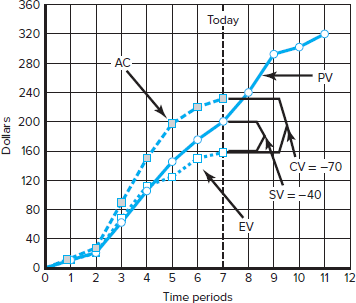
Figure 13.9 shows the graphed results of all the status reports through period 7. This graph represents the data from Table 13.2. The cumulative actual costs (AC) to page 491date and the earned value budgeted costs to date (EV) are plotted against the original project baseline (PV). The cumulative AC to date is $230; the cumulative EV to date is $160. Given these cumulative values, the cost variance (CV = EV − AC) is negative $70 (160 − 230 = −70). The schedule variance (SV = EV − PV) is negative $40 (160 − 200 = −40). Again, recall that only the project network or tracking Gantt chart can give an accurate assessment of schedule performance down to the work package level.
FIGURE 13.9
Digital Camera Prototype Summary Graph ($000)
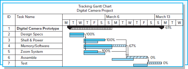
A tracking Gantt bar chart for the Digital Camera Prototype is shown in Figure 13.10. From this figure you can see Task C (Memory/Software), which had an original duration of four time units, now is expected to require six time units. This delay of two time units for Task C will also delay Tasks E and F two time units and result in the project being late two time periods.
FIGURE 13.10
Digital Camera Project-Tracking Gantt Chart Showing Status—through Period 7
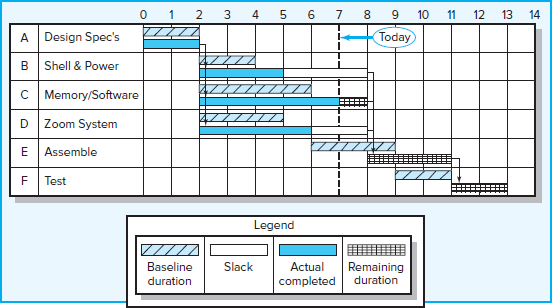
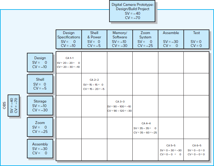
Figure 13.11 shows an oversimplified project rollup at the end of period 7. The rollup is by deliverables and organization units. For example, the Memory/Software deliverable has an SV of $ −10 and a CV of −30. The responsible “Storage” Department should have an explanation for these variances. Similarly, the Assembly Department, which is responsible for the Assemble and Test deliverables, has an SV of $ −30 due to the delay of Task C (see Figure 13.10). Most deliverables look unfavorable on schedule and cost variance.
FIGURE 13.11 Project Rollup End Period 7 ($000)
In more complex projects, the crosstabs of cost accounts by deliverables and organization units can be very revealing and more profound. This example contains the basics for developing a status report, developing baselines, and measuring schedule and cost variance. In our example, performance analysis had only one level above the cost account level. Because all data are derived from the detailed database, it is relatively easy to determine progress status at all levels of the work and organization breakdown structures. Fortunately, this same current database can provide additional views of the current status of the project and forecast costs at the completion of the project. Approaches for deriving additional information from the database are presented next.
To the uninitiated, a caveat is in order. In practice, budgets may not be expressed in total dollars for an activity. Frequently budgets are time-phased for materials and labor separately for more effective control over costs. Another common approach is to use labor hours in place of dollars in the earned value system. Later, labor hours are page 492converted to dollars. The use of labor hours in the earned value system is the modus operandi for most construction work. Labor hours are easy to understand and are often the way many time and cost estimates are developed. Most earned value software easily accommodates the use of labor hours for the development of cost estimates.
13.6 Indexes to Monitor Progress
Practitioners sometimes prefer to use schedule and cost indexes over the absolute values of SV and CV, because indexes can be considered efficiency ratios. Graphed indexes over the project life cycle can be very illuminating and useful. The trends are easily identified for deliverables and the whole project.
Indexes are typically used at the cost account level and above. In practice, the database is also used to develop indexes that allow the project manager and customer to view progress from several angles. An index of 1.00 (100 percent) indicates progress is as planned. An index greater than 1.00 shows progress is better than expected. An index less than 1.00 suggests progress is poorer than planned and deserves attention. Table 13.3 presents the interpretation of the indexes.
page 493
TABLE 13.3
Interpretation of Indexes
| Index | Cost (CPI) | Schedule (SPI) |
| >1.00 | Under cost | Ahead of schedule |
| =1.00 | On cost | On schedule |
| <1.00 | Over cost | Behind schedule |
Performance Indexes
There are two indexes of performance efficiency. The first index measures cost efficiency of the work accomplished to date (data from Table 13.2):

The CPI of .696 shows that $.70 worth of work planned to date has been completed for each $1.00 actually spent—an unfavorable situation indeed. The CPI is the most accepted and used index. It has been tested over time and found to be the most accurate, reliable, and stable. For example, U.S. government studies have shown that the CPI is stable from the 20 percent completion point regardless of contract type, program, or service. The CPI can provide an early warning signal as to cost overruns so that adjustments can be made to the budget or scope of a project.1
The second index is a measure of scheduling efficiency to date:

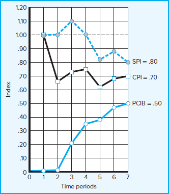
The schedule index indicates $.80 worth of work has been accomplished for each $1.00 worth of scheduled work to date. Figure 13.12 shows the indexes plotted for our example project through period 7. This figure is another example of graphs used in practice.
FIGURE 13.12
Indexes Periods 1–7
page 494
Project Percent Complete Indexes
Two project percent complete indexes are used, depending on your judgment of which one is most representative of your project. The first index assumes the original budget of work complete is the most reliable information to measure project percent complete. The second index assumes the actual costs-to-date and expected cost at completion are the most reliable for measuring project percent complete. These indexes compare the to-date progress to the end of the project. The implications underlying the use of these indexes are that conditions will not change, no improvement or action will be taken, and the information in the database is accurate. The first index looks at percent complete in terms of budget amounts:
Percent complete index budgeted costs

This PCIB indicates the work accomplished represents 50 percent of the total budgeted (BAC) dollars to date. Observe that this calculation does not include actual costs incurred. Because actual dollars spent do not guarantee project progress, this index is favored by many project managers when there is a high level of confidence in the original budget estimates.
The second index views percent complete in terms of actual dollars spent to accomplish the work to date and the actual expected dollars for the completed project (EAC). For example, at the end of period 7 the staff re-estimates that the EAC will be 575 instead of 320. The application of this view is written as
Percent complete index actual costs

Some managers favor this index because it contains actual and revised estimates that include newer, more complete information.
These two views of percent complete present alternative views of the “real” percent complete. These percents may be quite different, as shown. (Note: The PCIC index was not plotted in Figure 13.12. The new figures for EAC would be derived each period by estimators in the field.)
A third percent index that is popular in the construction industry reflects the amount of management reserves that has been absorbed by cost overruns. Remember that management reserves are funds set aside to cover unforeseen events (see Chapter 7). Let’s assume that $40 was reserved for the Digital Camera project:

The project has already spent 3 and half times the total funds set aside as management reserve. Clearly this project is in trouble and changes in either the scope or the budget are required. Many managers assess cost overruns in terms of management reserves rather than simply cost variance, since it reflects how much one can afford to spend on the project.
Software for Project Cost/Schedule Systems
Software developers have created sophisticated schedule/cost systems for projects that track and report budget, actual, earned, committed, and index values. These values can be labor hours, materials, and/or dollars. This information supports cost and schedule progress, performance measurements, and cash flow management. page 495Recall from Chapter 5 that budget, actual, and committed dollars usually run in different time frames (see Figure 5.6). A typical computer-generated status report includes the following information outputs:
Schedule variance (EV − PV) by cost account and WBS and OBS.
Cost variance (EV − AC) by cost account and WBS and OBS.
Indexes—total percent complete and performance index.
Cumulative actual total cost to date (AC).
Expected costs at completion (EAC).
Paid and unpaid commitments.
The variety of software packages, with their features and constant updating, is too extensive for inclusion in this text. Software developers and vendors have done a superb job of providing software to meet the information needs of most project managers. Differences among software in the last decade have centered on improving “friendliness” and output that is clear and easy to understand. Anyone who understands the concepts and tools presented in Chapters 4, 5, 6, 8, and 13 should have little trouble understanding the output of any of the popular project management software packages. Appendix 13.2 details how to obtain earned value information from Microsoft Project software.
Additional Earned Value Rules
Although the percent complete rule is the most-used method of assigning budgets to baselines and for cost control, there are additional rules that are very useful for reducing the overhead costs of collecting detailed data on percent complete of individual work packages. (An additional advantage of these rules, of course, is that they remove the often subjective judgments of the contractors or estimators as to how much work has actually been completed.) The first two rules are typically used for short-duration activities and/or small-cost activities. The third rule uses gates before the total budgeted value of an activity can be claimed.
0/100 rule. This rule assumes credit is earned for having performed the work once it is completed. Hence, 100 percent of the budget is earned when the work package is completed. This rule is used for work packages having very short durations.
50/50 rule. This approach allows 50 percent of the value of the work package budget to be earned when it is started and 50 percent to be earned when the package is completed. This rule is popular for work packages of short duration and small total costs.
Percent complete with weighted monitoring gates. This more recent rule uses subjective estimated percent complete in combination with hard, tangible monitoring points. This method works well on long-duration activities that can be broken into short, discrete work packages of no more than one or two report periods. These discrete packages limit the subjective estimated values. For example, assume a long-duration activity with a total budget of $500. The activity is cut into three sequentially discrete packages with monitoring gates representing 30, 50, and 100 percent of the total budget. The earned amount at each monitoring gate cannot exceed $150, $250, and $500. These hard monitoring points serve as a check on overly optimistic estimates.
Notice the only information needed for the first two rules is that the work package has started and the package has been completed. Appendix 13.1 presents two exercises that apply these rules along with the percent complete rule.
page 496
The third rule is frequently used to authorize progress payments to contractors. This rule supports careful tracking and control of payments; it discourages payment to contractors for work not yet completed.
13.7 Forecasting Final Project Cost
There are basically two methods used to revise estimates of future project costs. In many cases both methods are used on specific segments of the project. The result is confusion of terms in texts, in software, and among practitioners in the field. We have chosen to note the differences between the methods.
The first method allows experts in the field to change original baseline durations and costs because new information tells them the original estimates are not accurate. We have used EACre to represent revisions made by experts and practitioners associated with the project. The revisions from project experts are almost always used on smaller projects.
The equation for calculating revised estimated cost at completion (EACre) is as follows:

where
| EACre | = | revised estimated cost at completion. |
| AC | = | cumulative actual cost of work completed to date. |
| ETCre | = | revised estimated cost to complete remaining work. |
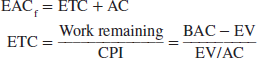
A second method is used in large projects where the original budget is reliable. This method uses the actual costs to date plus an efficiency index (CPI = EV/AC) applied to the remaining project work. When the estimate for completion uses the CPI as the basis for forecasting cost at completion, we use the acronym EACf. The equation for this forecasting model (EACf) is as follows:
where
| EACf | = | forecasted total cost at completion. |
| ETC | = | estimated cost to complete remaining work. |
| AC | = | cumulative actual cost of work completed to date. |
| CPI | = | cumulative cost index to date. |
| BAC | = | total budget of the baseline. |
| EV | = | cumulative budgeted cost of work completed to date. |
The following information is available from our earlier example; the estimated cost at completion (EACf) is computed as follows:
| Total baseline budget (BAC) for the project | $320 |
| Cumulative earned value (EV) to date | $160 |
| Cumulative actual cost (AC) to date | $230 |
page 497
The final project projected cost forecast is $459,000 versus $320,000 originally planned.
Another popular index is the To complete performance index (TCPI), which is useful as a supplement to the estimate at complete (EACf) computation. This ratio measures the amount of value each remaining dollar in the budget must earn to stay within the budget. The index is computed for the Digital Camera project at the end of period 7:

The index of 1.78 indicates that each remaining dollar in the budget must earn $1.78 in value in order for the project to stay within budget. There is more work to be done than there is budget left. Clearly it would be tough to increase productivity that much to make budget. The work to be done will have to be reduced, or you will have to accept running over budget. If the TCPI is less than 1.00, you should be able to complete the project without using all of the remaining budget. A ratio of less than 1.00 opens the possibility of other opportunities such as improving quality, increasing profit, or expanding scope.
Research data indicate that on large projects that are more than 15 percent complete, the model performs well with an error of less than 10 percent (Christensen, 1998; Fleming & Koppleman, 2010). This model can also be used for WBS and OBS cost accounts that have been used to forecast remaining and total costs. It is important to note that this model assumes conditions will not change, the cost database is reliable, EV and AC are cumulative, and past project progress is representative of future progress. This objective forecast represents a good starting point or benchmark that management can use to compare other forecasts that include other conditions and subjective judgments.
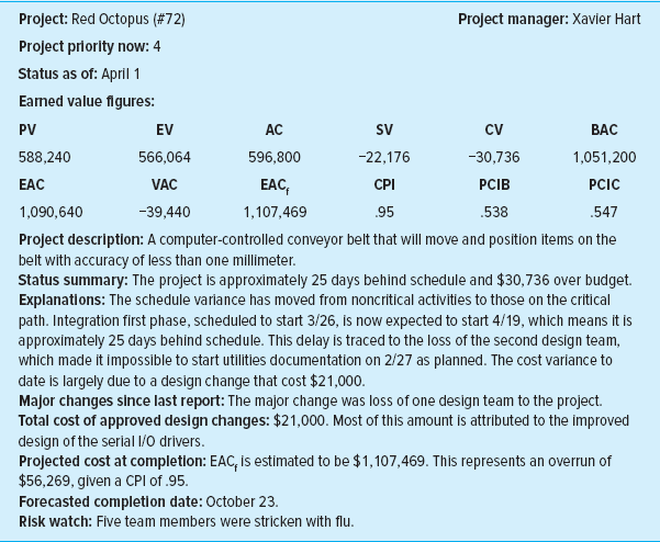
Exhibit 13.1 presents an abridged monthly status report similar to one used by a project organization. The form is used for all projects in their project portfolio. page 498(Note that the schedule variance of −$22,176 does not translate directly to days. The 25 days were derived from the network schedule.)
EXHIBIT 13.1
Monthly Status Report
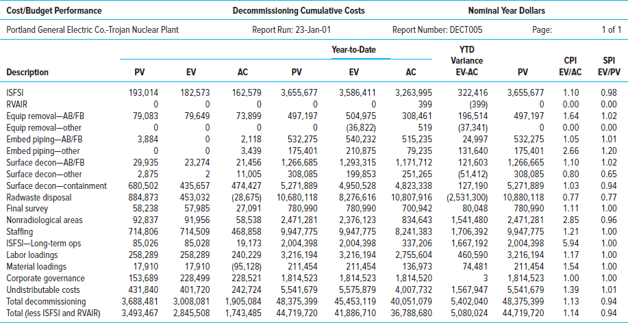
Another summary report is shown in Snapshot from Practice 13.2: Trojan Decommissioning Project. Compare the differences in format.
13.8 Other Control Issues
Technical Performance Measurement
Measuring technical performance is as important as measuring schedule and cost performance. Although technical performance is often assumed, the opposite can be true. The ramifications of poor technical performance frequently are more profound—something works or it doesn’t if technical specifications are not adhered to.
Assessing technical performance of a system, facility, or product is often accomplished by examining the documents found in the scope statement and/or work package documentation. These documents should specify criteria and tolerance limits against which performance can be measured. For example, the technical performance of a software project suffered because the feature of “drag and drop” was deleted in the final product. Conversely the prototype of an experimental car exceeded the miles per gallon technical specification and, thus, its technical performance. Frequently tests are conducted on different performance dimensions. These tests become an integral part of the project schedule.
It is very difficult to specify how to measure technical performance because it depends on the nature of the project. Suffice it to say, measuring technical performance must be done. Technical performance is frequently where quality control processes are needed and used. Project managers must be creative in finding ways to control this very important area.
page 499
EXHIBIT 13.2
page 500
Scope Creep
Large changes in scope are easily identified. It is the “minor refinements” that eventually build to be major scope changes that can cause problems. These small refinements are known in the field as scope creep. For example, the customer of a software developer requested small changes in the development of a custom accounting software package. After several minor refinements, it became apparent the changes represented a significant enlargement of the original project scope. The result was an unhappy customer and a development firm that lost money and reputation.
Although scope changes are usually viewed negatively, there are situations when scope changes result in positive rewards. Scope changes can represent significant opportunities.2 In product development environments, adding a small feature to a product can result in a huge competitive advantage. A small change in the production process may get the product to market one month early or reduce product cost.
Scope creep is common early in projects—especially in new-product development projects. Customer requirements for additional features, new technology, poor design assumptions, and so on, all manifest pressures for scope changes. Frequently these changes are small and go unnoticed until time delays or cost overruns are observed. Scope creep affects the organization, project team, and project suppliers. Scope changes alter the organization’s cash flow requirements in the form of fewer or additional resources, which may also affect other projects. Frequent changes eventually wear down team motivation and cohesiveness. Clear team goals are altered, become less focused, and cease being the focal point for team action. Starting over again is annoying and demoralizing to the project team because it disrupts project rhythm and lowers productivity. Project suppliers resent frequent changes because they represent higher costs and have the same effect on their team as on the project team.
The key to managing scope creep is change management. One project manager of an architectural firm related that scope creep was the biggest risk his firm faced in projects. The best defense against scope creep is a well-defined scope statement. Poor scope statements are one of the major causes of scope creep.
A second defense against scope creep is stating what the project is not, which can avoid misinterpretations later. (Chapter 7 discusses the process. See Figure 7.9 to review key variables to document in project changes.) First, the original baseline must be well defined and agreed upon with the project customer. Before the project begins, it is imperative that clear procedures be in place for authorizing and documenting scope changes by the customer or project team. If a scope change is necessary, the impact on the baseline should be clearly documented—for example, cost, time, dependencies, specifications, or responsibilities. Finally, the scope change must be quickly added to the original baseline to reflect the change in budget and schedule; these changes and their impacts need to be communicated to all project stakeholders.
Baseline Changes
Changes during the life cycle of projects are inevitable. Some changes can be very beneficial to project outcomes; changes having a negative impact are the ones we wish to avoid. Careful project definition can minimize the need for changes. The price for poor project definition can be changes that result in cost overruns, late schedules, low morale, and loss of control. Change comes from external sources or from within. Externally, for example, the customer may request changes that were not included in the original scope statement and that will require significant changes to the project and page 501thus to the baseline. Or the government may render requirements that were not a part of the original plan and that require a revision of the project scope. Internally, stakeholders may identify unforeseen problems or improvements that change the scope of the project. In rare cases scope changes can come from several sources. For example, the Denver International Airport automatic baggage handling system was an afterthought supported by several project stakeholders that included the Denver city government, consultants, and at least one airline customer. The additional $2 billion in costs were staggering, and the airport opening was delayed 16 months. If this automatic baggage scope change had been in the original plan, costs would have been only a fraction of the overrun costs, and delays would have been reduced significantly. Any changes in scope or the baseline should be recorded by the change management system that was set in place during risk control planning. (See Chapter 7.)
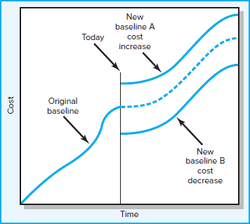
Generally project managers monitor scope changes very carefully. They should allow scope changes only if it is clear that the project will fail without the change, the project will be improved significantly with the change, or the customer wants it and will pay for it. This statement is an exaggeration, but it sets the tone for approaching baseline changes. The effect of the change on the scope and baseline should be accepted and signed off by the project customer. Figure 13.13 depicts the cost impact of a scope change on the baseline at a point in time—“today.” Line A represents a scope change that results in an increase in cost. Line B represents a scope change that decreases cost. Quickly recording scope changes to the baseline keeps the computed earned values valid. Failure to do so results in misleading cost and schedule variances.
FIGURE 13.13
Scope Changes to a Baseline
Care should be taken to not use baseline changes to disguise poor performance on past or current work. A common signal of this type of baseline change is a constantly revised baseline that seems to match results. Practitioners call this a “rubber baseline” because it stretches to match results. Most changes will not result in serious scope changes and should be absorbed as positive or negative variances. Retroactive changes for work already accomplished should not be allowed. Transfer of money among cost accounts should not be allowed after the work is complete. Unforeseen changes can page 502be handled through the contingency reserve. The project manager typically makes this decision. In some large projects, a partnering “change review team,” made up of members of the project and customer teams, makes all decisions on project changes.
The Costs and Problems of Data Acquisition
Data acquisition is time consuming and costly. Snapshot from Practice 13.3: A Pseudo-Earned Value Percent Complete Approach captures some of the frequent issues surrounding resistance to data collection of percent complete for earned value systems. Similar pseudo-percent complete systems have been used by others. Such pseudo-percent complete approaches appear to work well in multiproject environments that include several small and medium-sized projects. Assuming a one-week reporting period, care needs to be taken to develop work packages with a duration of about one week long so problems are identified quickly. For large projects, there is no substitute for using a percent complete system that depends on data collected through observation at clearly defined monitoring points.
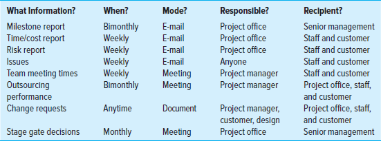
In some cases data exist but are not sent to the stakeholders who need information relating to project progress. Clearly if the information does not reach the right people in a timely manner, you can expect serious problems. Your communication plan developed in the project planning stage can greatly mitigate this problem by mapping out the flow of information and keeping stakeholders informed on all aspects of project progress and issues. See Figure 13.14 for an internal communication plan for a WiFi project. The information developed in this chapter contributes significant data to support your communication plan and ensures correct dissemination of the data.
page 503
FIGURE 13.14
Conference Center WiFi Project Communication Plan
Summary
The best information system does not result in good control. Control requires the project manager to use information to steer the project through rough waters. Control and Gantt charts are useful vehicles for monitoring time performance. Earned Value Management (EVM) allows the manager to have a positive influence on cost and schedule in a timely manner. The ability to influence cost decreases with time; therefore, timely reports identifying adverse cost trends can greatly assist the project manager in getting back on budget and schedule. EVM provides the project manager and other stakeholders with a snapshot of the current and future status of the project. The benefits of EVM are as follows:
Measures accomplishments against plan and deliverables.
Provides a method for tracking directly to a problem work package and organization unit responsible.
Alerts all stakeholders to early identification of problems and allows for quick, proactive corrective action.
Improves communication because all stakeholders are using the same database.
Keeps customers informed of progress and encourages customer confidence that the money spent is resulting in the expected progress.
6.Provides for accountability over individual portions of the overall budget for each organization unit.
Key Terms
Review Questions
How does a tracking Gantt chart help communicate project progress?
How does earned value give a clearer picture of project schedule and cost status than a simple plan versus actual system?
page 504 Schedule variance (SV) is in dollars and does not directly represent time. Why is it still useful?
How would a project manager use the CPI?
What are the differences between BAC and EAC?
Why is it important for project managers to resist changes to the project baseline? Under what conditions would a project manager make changes to a baseline? When would a project manager not allow changes to a baseline?
SNAPSHOT  FROM PRACTICE
Discussion Questions
13.1 Guidelines for Setting Milestones
Why should a milestone be a concrete, specific, measurable event?
Should milestones only be on the critical path?
13.2 Trojan Decommissioning Project
Based on the information provided in Exhibit 13.2, how well is the Decommissioning project doing in terms of cost and schedule?
What additional information would you like to have in order to assess performance on the project?
13.3 A Pseudo-Earned Value Percent Complete Approach
How did limiting work packages to one week help management identify problems sooner?
Why do organizations use the percent complete instead of the cheaper, easier pseudo-earned value percent approach?
Exercises
In month 9 the following project information is available: actual cost is $2,000, earned value is $2,100, and planned cost is $2,400. Compute the SV and CV for the project.
On day 51 a project has an earned value of $600, an actual cost of $650, and a planned cost of $560. Compute the SV, CV, and CPI for the project. What is your assessment of the project on day 51?
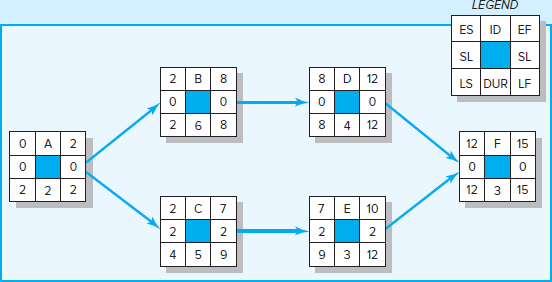
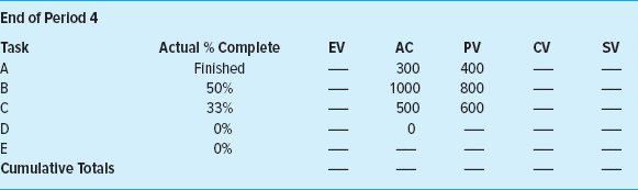
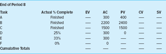
Given the following project network and baseline information, complete the form to develop a status report for the project at the end of period 4 and the end of period 8. From the data you have collected and computed for periods 4 and 8, what information are you prepared to tell the customer about the status of the project at the end of period 8?
page 505

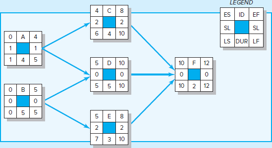
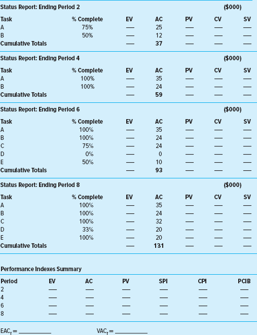
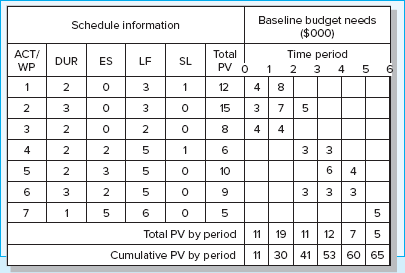
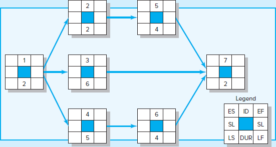
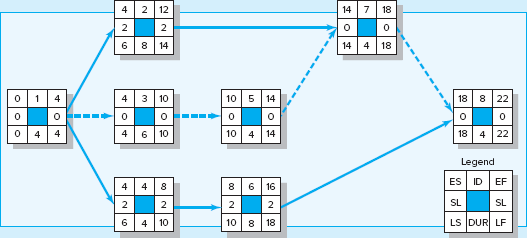
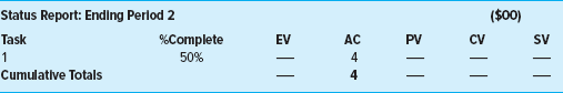
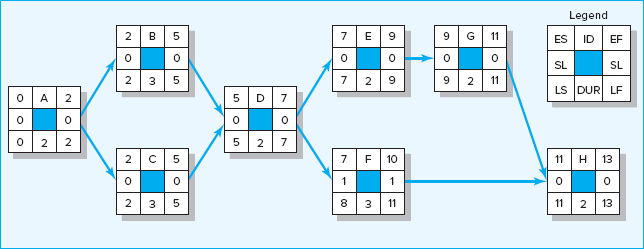
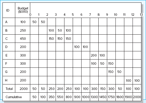
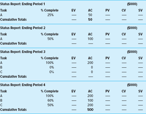
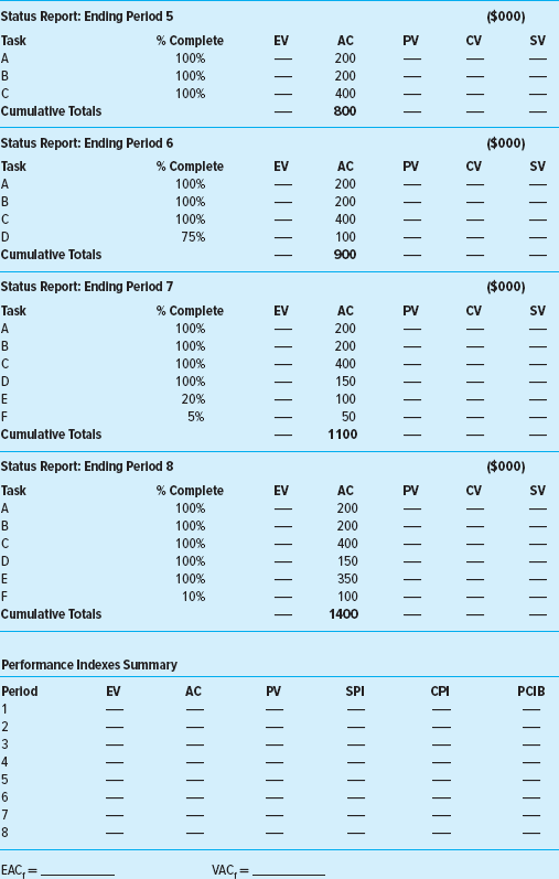
page 506Given the following project network, baseline, and status information, develop status reports for periods 2, 4, 6, 8 and complete the performance indexes table. Calculate the EACf and the VACf. Based on your data, what is your assessment of the current status of the project? At completion?
page 507
page 508 Given the following project network, baseline, and status information, develop status reports for periods 1–4 and complete the project summary graph (or a similar one). Report the final SV, CV, CPI, and PCIB. Based on your data, what is your assessment of the current status of the project? At completion?

page 509


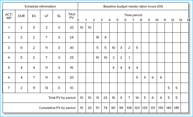
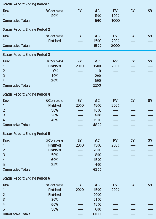
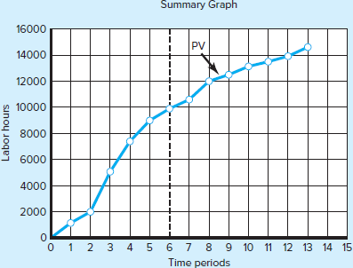
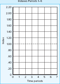
page 510 The following labor hours data have been collected for a nanotechnology project for periods 1 through 6. Compute the SV, CV, SPI, and CPI for each period. Plot the EV and the AC on the summary graph provided (or a similar one). Plot the SPI, CPI, and PCIB on the index graph provided (or a similar one). What is your assessment of the project at the end of period 6?
page 511
page 512
Period SPI CPI PCIB 1
2
3
4
5
6
—
—
—
—
—
—
—
—
—
—
—
—
—
—
—
—
—
—
SPI = EV/PV
CPI = EV/AC
PCIB = EV/BAC
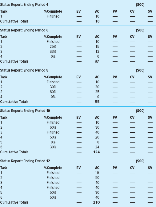
page 513 The following data have been collected for a British healthcare IT project for two-week reporting periods 2 through 12. Compute the SV, CV, SPI, and CPI for each period. Plot the EV and the AC on the summary graph provided. Plot the SPI, CPI, and PCIB on the index graph provided. (You may use your own graphs.) What is your assessment of the project at the end of period 12?

page 514
Period SPI CPI PCIB 2
4
6
8
10
12
—
—
—
—
—
—
—
—
—
—
—
—
—
—
—
—
—
—
SPI = EV/PV
CPI = EV/AC
PCIB = EV/BAC
page 515

Part A.* You are in charge of the Aurora project. Given the following project network, baseline, and status information, develop status reports for periods 1–8 and complete the performance indexes table. Calculate the EACf and VACf. Based on your data, what is the current status of the project? At completion?
page 516
page 517
page 518
Part B. You have met with your Aurora project team and they have provided you with the following revised estimates for the remainder of the project:
Activity F will be completed at the end of period 12 at a total cost of $500.
Activity G will be completed at the end of period 10 at a total cost of $150.
Activity H will be completed at the end of period 14 at a total cost of $200.
Calculate the EACre and VACre. Based on the revised estimates, what is the expected status of the project in terms of cost and schedule? Between the VACf and the VACre, which one would you have the greatest confidence in?
EACre = _________________VACre = _________________
References
Abramovici, A., “Controlling Scope Creep,” PM Network, January 2000, pp. 44–48.
Anbari, F. T., “Earned Value Project Management Method and Extensions,” Project Management Journal, vol. 34, no. 4 (December 2003), pp. 12–22.
Bowles, M. “Keeping Score,” PM Network, May 2011, pp. 50–59.
Brandon, D. M., Jr., “Implementing Earned Value Easily and Effectively,” Project Management Journal, vol. 29, no. 3 (June 1998), pp. 11–17.
Christensen, D. S., “The Cost and Benefits of the Earned Value Management Process,” Acquisition Review Quarterly, vol. 5 (1998), pp. 373–86.
Christensen, D. S., and S. Heise, “Cost Performance Index Stability,” National Contract Management Association Journal, vol. 25 (1993), pp. 7–15.
Fleming, Q., and Joel M. Koppelman, Earned Value Project Management, 4th ed. (Newton Square, PA: Project Management Institute, 2010).
Kerzner, H., “Strategic Planning for a Project Office,” Project Management Journal, vol. 34, no. 2 (June 2003), pp. 13–25.
Kim, E. H., W. G. Wells, and M. R. Duffey, “A Model for Effective Implementation of Earned Value Methodology,” International Journal of Project Management, vol. 21, no. 5 (2003), pp. 375–82.
Naeni, L., S. Shadrokh, and A. Salehipour, “A Fuzzy Approach to the Earned Value Management,” International Journal of Project Management, vol. 9, no. 6 (2011), pp. 764–72.
Webb, A., Using Earned Value: A Project Manager’s Guide (Aldershot, UK: Gower, 2003).
* The solution to this exercise can be found in Appendix One.
page 519
Case 13.1
Tree Trimming Project
Wil Fence is a large timber and Christmas tree farmer who is attending a project management class in the spring, his off season. When the class topic came to earned value, he was perplexed. Isn’t he using EV?
Each summer Wil hires crews to shear fields of Christmas trees for the coming holiday season. Shearing entails having a worker use a large machete to shear the branches of the tree into a nice, cone-shaped tree.
Wil describes his business as follows:
I count the number of Douglas Fir Christmas trees in the field (24,000).
Next, I agree on a contract lump sum for shearing with a crew boss for the whole field ($30,000).
When partial payment for work completed arrives (5 days later), I count or estimate the actual number sheared (6,000 trees). I take the actual as a percent of the total to be sheared and multiply the percent complete by total contract amount for the partial payment [(6,000/$30,000 = 25%), (.25 × $30,000 = $7500)].
Is Wil over, on, or below cost and schedule? Is Wil using earned value?
How can Wil set up a scheduling variance?
Case 13.2
Ventura Stadium Status Report Case
You are an assistant to Percival Young, president of G&E Company. He has asked you to prepare a brief report on the status of the Ventura Stadium project.
Ventura Stadium is a 47,000-seat professional baseball stadium. Construction started on July 8, 2019, and the stadium is to be completed on February 21, 2022. The project is estimated to cost $320,000,000. There are $35 million management reserves to deal with unexpected problems and delays.
The stadium must be ready for the 2022 major league season. G&E would accrue a $500,000 per day penalty for not meeting the April 3, 2022, deadline.
It is February 25, 2021, the day crews start installing seats.
Tables C13.1 and C13.2 contain information submitted by your counterpart at the Ventura site from which you are to prepare your report. Use the appropriate indexes/information to prepare a report informing Mr. Young on the overall status of the Ventura project in terms of costs and schedule. Note: Mr. Young is not interested in specifics, just how well the overall project is doing and if there is a need to take corrective action.
page 520
TABLE C13.1 Ventura Project Earned Value Table as of 2/25/21

|
TABLE C13.2 Variance Table for Ventura Project as of 2/25/21

|
page 521
Case 13.3
Scanner Project
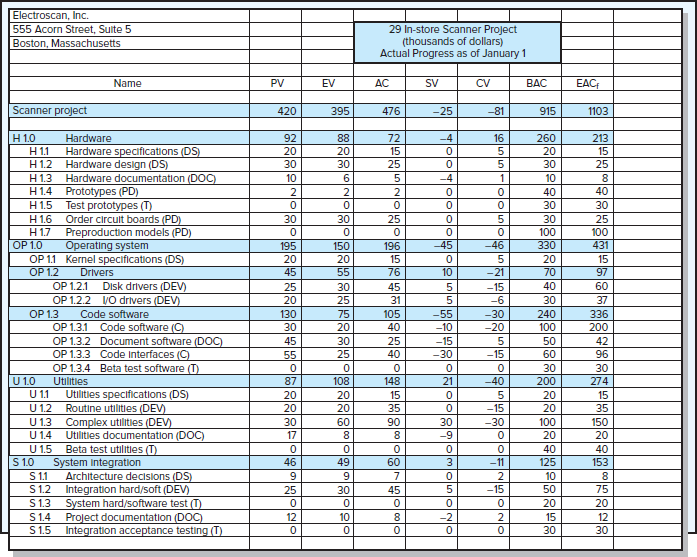
You have been serving as Electroscan’s project manager and are now well along in the project. Develop a narrative status report for the board of directors of the chain store that discusses the status of the project to date (see Table C13.3) and at completion. Be as specific as you can, using the numbers given and those you might develop. Remember, your audience is not familiar with the jargon used by project managers and computer software personnel; therefore, some explanation may be necessary. Your report will be evaluated on your detailed use of the data, your total perspective of the current status and future status of the project, and your recommended changes (if any).
TABLE C13.3
|
page 522
Appendix 13.1
The Application of Additional Earned Value Rules
The following example and exercises are designed to provide practice in applying the following three earned value rules:
Percent complete rule
50/50 rule
0/100 rule
See the chapter for an explanation of each of these rules.
Simplifying Assumptions
The same simplifying assumptions used for the chapter example and exercises will also be used here.
Assume each cost account has only one work package, and each cost account will be represented as an activity on the network.
The project network early start times will serve as the basis for assigning the baseline values.
Except when the 0/100 rule or 50/50 rule is used, baseline values will be assigned linearly, unless stated differently. (Note: In practice, estimated costs should be applied “exactly” as they are expected to occur so measures of schedule and cost performance are useful and reliable.)
For purposes of demonstrating the examples, from the moment work on an activity begins, some actual costs will be incurred each period until the activity is completed.
When the 0/100 rule is used, the total cost for the activity is placed in the baseline on the early finish date.
When the 50/50 rule is used, 50 percent of the total cost is placed in the baseline on the early start date and 50 percent on the early finish date.
Appendix Exercises
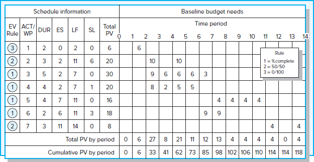
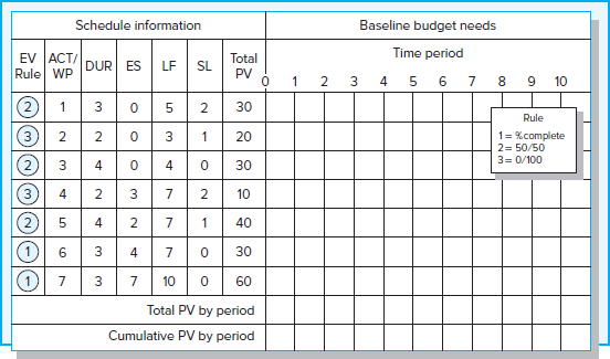
Given the information provided for development of a product warranty project for periods 1 through 7, compute the SV, CV, SPI, and CPI for each period. Figure A13.1-1A presents the project network. Figure A13.1-1B presents the project baseline, noting those activities using the 0/100 (rule 3) and 50/50 (rule 2) rules. For example, activity 1 uses rule 3, the 0/100 rule. Although the early start time is period 0, the budget is not placed in the time-phased baseline until period 2 when the activity is planned to be finished (EF). This same procedure has been used to assign costs for activities 2 and 7. Activities 2 and 7 use the 50/50 rule. Thus, 50 percent of the budget for each activity is assigned on its respective early start page 523date (time period 2 for activity 2 and period 11 for activity 7) and 50 percent for their respective finish dates. Remember, when assigning earned value as the project is being implemented, if an activity actually starts early or late, the earned values must shift with the actual times. For example, if activity 7 actually starts in period 12 rather than 11, the 50 percent is not earned until period 12.
FIGURE A13.1-1A

FIGURE A13.1-1B
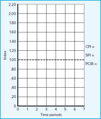
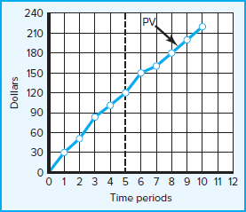
Plot the EV and the AC on the PV graph provided (Figure A13.1-1D). Use Figure A13.1-1C. to plot the CPI, PI, and PCIB. Explain to the owner your assessment of the project at the end of period 7 and the future expected status of the project at completion.
FIGURE A13.1-1C
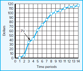
FIGURE A13.1-1D
page 524

page 525
Period SPI CPI PCIB 1
2
3
4
5
6
7
—
—
—
—
—
—
—
—
—
—
—
—
—
—
—
—
—
—
—
—
—
SPI = EV/PV
CPI = EV/AC
PCIB = EV/BAC
Given the information provided for development of a catalog product return process for periods 1 through 5, assign the PV values (using the rules) to develop a baseline for the project. Compute the SV, CV, SPI, and CPI for each period. Assume that PV will be evenly distributed across the activity’s duration. Explain to the owner your assessment of the project at the end of period 5 and the future expected status of the project at the completion.
page 526
FIGURE A13.1-2A

FIGURE A13.1-2B
page 527
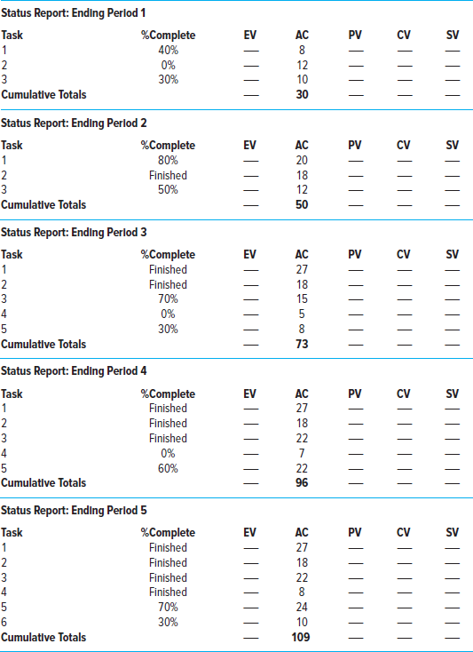
FIGURE A13.1-2C
page 528
Period SPI CPI PCIB 1
2
3
4
5
—
—
—
—
—
—
—
—
—
—
—
—
—
—
—
SPI = EV/PV
CPI = EV/AC
PCIB = EV/BAC
Appendix 13.2
Obtaining project performance information from MS Project 2010 or 2016.
The objective of this appendix is to illustrate how one can obtain the performance information discussed in Chapter 13 from MS Project 2010 or 2016. One of the great strengths of MS Project is its flexibility. The software provides numerous options for entering, calculating, and presenting project information. Flexibility is also the software’s greatest weakness in that there are so many options that working with the software can be frustrating and confusing. The intent here is to keep it simple and present basic steps for obtaining performance information. Students with more ambitious agendas are advised to work with the software tutorial or consult one of many instructional books on the market.
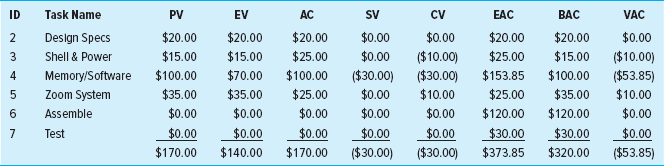
For purposes of this exercise we will use the Digital Camera project, which was introduced in Chapter 13. In this scenario the project started as planned on March 1 and today’s date is March 7. We have received the following information on the work completed to date:
Design Specs took 2 days to complete at a total cost of $20.
Shell & Power took 3 days to complete at a total cost of $25.
Memory/Software is in progress with 4 days completed and 2 days remaining.
Cost to date is $100.
Zoom System took 2 days to complete at a cost of $25.
All tasks started on time.
page 529
STEP 1 ENTERING PROGRESS INFORMATION
We enter this progress information in the TRACKING TABLE from the GANTT CHART VIEW ▶ VIEW ▶ TABLES ▶ TRACKING:
TABLE A13.2-1A Tracking Table

|
Note that the software automatically calculates the percent complete and actual finish, cost, and work. In some cases you will have to override these calculations if they are inconsistent with what actually happened. Be sure to check to make sure the information in this table is displayed the way you want it to be.
The final step is to enter the current status date (March 7). You do so by clicking PROJECT ▶ PROJECT INFORMATION and inserting the date into the status date window.
STEP 2 ACCESSING PROGRESS INFORMATION
MS Project provides a number of different options for obtaining progress information. The most basic information can be obtained from PROJECT ▶ REPORTS ▶ COSTS ▶ EARNED VALUE. You can also obtain this information from GANTT CHART view. Click VIEW ▶ TABLE ▶ MORE TABLES ▶ EARNED VALUE.
TABLE A13.2-1B Earned Value Table
|
page 530
When you scale this table to 80 percent you can obtain all the basic CV, SV, and VAC information on one convenient page.
Note: Some versions of MS Project use the old acronyms:
BCWS = PV
BCWP = EV
ACWP = AC
and the EAC is calculated using the CPI and is what the text refers to as EACf.
STEP 3 ACCESSING CPI INFORMATION
To obtain additional cost information such as CPI and TCPI from the GANTT CHART view, click VIEW ▶ TABLE ▶ MORE TABLES ▶ EARNED VALUE COST INDICATORS, which will display the following information:
TABLE A13.2-1C Earned Value Cost Indicators Table
|
Note: For MS Project 2007 users the instructions are very similar except you can access the Tables option directly from GANTT View.
STEP 4 ACCESSING SPI INFORMATION
To obtain additional schedule information such as SPI from the GANTT CHART view, click VIEW ▶ TABLE ▶ MORE TABLES ▶ EARNED VALUE SCHEDULE INDICATORS, which will display the following information:
TABLE A13.2-1D
Earned Value Schedule Indicators Table
|
page 531
STEP 5 CREATING A TRACKING GANTT CHART
You can create a tracking Gantt chart like the one presented in Figure 13.1 by simply clicking TASK ▶ GANTT CHART (upper left-hand corner) ▶ TRACKING GANTT ▶ TRACKING GANTT.
FIGURE A13.2-1E
Tracking Gantt Chart
Design elements: Snapshot from Practice, Highlight box, Case icon: ©Sky Designs/Shutterstock
1 Cited by Fleming, Q. W., and J. M. Koppleman, Earned Value Project Management (Newton Square, PA: Project Management Institute, 2010), pp. 39–42.
2 See: Keifer, S. “Scope Creep . . . Not Necessarily a Bad Thing,” PM Network, May 1996, pp. 33–35.