Signal Detection Theory
This chapter will mostly concern the use of signal detection theory to analyze data generated in psychophysical—and hypothetical neurophysiological—experiments. We will do this in MATLAB®.
Keywords
criterion; significance level; fundamental error; false positive; false negative
10.1 Goals of This Chapter
This chapter will mostly concern the use of signal detection theory to analyze data generated in psychophysical—and hypothetical neurophysiological—experiments. As usual, we will do this in MATLAB®.
10.2 Background
At its core, signal detection theory (SDT) represents a way to optimally detect a signal in purely statistical terms without an explicit link to decision processes in particular or cognitive processes in general. However, in the context of our discussion, SDT provides a rich view of the problem of how to detect a given signal. It reframes the task as a decision process, adding a cognitive dimension to our understanding of this matter.
To illustrate the application of SDT in psychophysics, let us again consider the problem of reporting the presence or absence of a faint, barely visible dot of light, as in Chapter 8, “Psychophysics.” In addition to the threshold, which is determined by the physical properties of the stimuli and the physiological properties of the biological substrate, there are cognitive considerations. In particular, observers have a criterion by which they judge (and report) whether or not a signal was present. Many factors can influence the criterion level and—hence—this report. You likely encountered some of those in the preceding chapters. For example, your criterion levels might have been influenced by doing a couple hundred trials, giving you an appreciation of what “present” and “absent” mean in the context of the given stimulus range (which is very dim overall). Moreover, motivational concerns might play a role when setting a criterion level. If research participants have an incentive to over- or under-report the presence of a signal—e.g., if they think that the experimenter expects this—they will in fact do so (Rosenthal, 1976). Interestingly, neuroeconomists utilize this effect by literally paying their research participants to prefer one alternative, in order to study the mechanisms of how the criterion level is set.
Of course, one could question the real-world relevance of these considerations, given that they arose in very particular and arguably often rather contrived experimental settings. It is worth emphasizing that this first impression is extremely misleading. Today, signal detection theory constitutes a formal, stochastic way to estimate the probability by which some things are the case and others are not; by which some effects are real and others are not, and so on. As such, it has the broadest possible implications. Signal detection theory is used by pharmaceutical companies as well as oil prospectors, and it has even made its mark in public policy considerations. Of course, experimenters—psychophysicists in particular—also still use it.
The astonishing versatility and base utility of signal detection theory are likely owed to the fact that it goes to the very heart of what it means to be a cognitive organism or system, as we will now describe.
Consider the following situation. Let us assume you work for a company that builds and installs fire alarm systems. As these systems are ubiquitous in modern cities, business is good. However, you are confronted with a rather confounding problem: How sensitive should you make these alarms? The four possible cases are tabulated in a classic matrix, as shown in Table 10.1.
Table 10.1
The Signal Detection Theory Payoff Matrix
| Real fire | No fire (but possibly some smoke or heat) | |
| Alarm goes off | Hit | False alarm |
| Alarm does not go off | Miss | Correct rejection |
Let’s peruse this matrix in detail as it is the foundation of the entire discussion to follow. The cell in the upper left represents the “desired” (as desired as it can be, given that there is a real fire in the building) case: there actually is a fire and the alarm does go off, urging the occupants of the building to leave and alerting the fire department to the situation. Ideally, you would like the probability of this event to be 1. In other words, you always want the alarm to go off when there is a fire present. This part should be fairly uncontroversial. The problem is that in order to reach a probability of 1 for this case, you need to set the criterion level for indicating “fire” by some parameters (usually smoke or heat or both) incredibly low. In fact, you need to set it so low that it will likely go off by levels of smoke or heat that can be reached without a fire being present. This puts you into the cell in the upper right. If this happens, you have a false alarm. From personal experience, you can probably confirm that the criterion levels of fire alarms are typically set in a hair-trigger fashion. Almost anything will set them off, and almost all alarms are therefore false alarms, given that the a priori probability of a real fire is very, very low. As is the case in modern cities. While this situation is better than having a real fire, false alarms are not trivial. Having them frequently is disruptive, can potentially have deleterious effects in case of a real fire (as the occupants of the building learn to stop taking action when the alarm goes off), and strains the resources of the firefighters (as a matter of fact, firefighters have been killed in traffic accidents on their way to false alarms). In other words, setting the sensitivity too high comes at a considerable cost. Hence, you want to lower the sensitivity enough to always be in a state that corresponds to one of the cells on the main diagonal of the matrix, either having a hit (if there is actually a fire present) or a “correct rejection,” arriving in the lower right. The latter should be the most common case, indicating that there is no fire and the fire alarm does not go off. Unfortunately, if you drop the sensitivity too low, you arrive in the worst cell of all in terms of potential for damage and fatalities: having a real fire, but the fire alarm does not alert you to this situation. This is called a “miss,” in the lower left.
In a way, this matrix illustrates what signal detection theory is all about: figuring out a way to set the criterion in a mathematically optimal fashion (in the applied version) and figuring out how and why people, organisms, and systems actually do set criteria when performing and solving cognitive tasks (in the pure research version).
If this description sounds familiar, it should. As contemporary science has largely adopted a stochastic view on epistemology, this fundamental situation of signal detection theory appears in many if not most experiments, disguised as the “p-value” problem.
You are probably well aware of this issue, so let us just briefly retrace it in terms of signal detection theory.
When performing an experiment, you observe a certain pattern of results. The basic question is always: How likely is this pattern, given there is no effect of experimental manipulation? In other words: How likely are the observed data to occur purely by chance? If they are too unlikely given chance alone, you reject the “null hypothesis” that the data came about by chance alone. That is—in a nutshell—the fundamental logic of testing for the statistical significance of most experimental data since Fisher introduced and popularized the concept in the 1920s (Fisher, 1925).
But how unlikely is too unlikely? Again, we face the fundamental signal detection dilemma, as illustrated in Table 10.2.
Table 10.2
Alpha and Beta Errors in Experimental Judgment
| Effect exists (H0 false) | Effect does not exist (H0 true) | |
| We conclude it exists | Discovery of effect | Alpha error (false rejection of H0) |
| We conclude it doesn’t exist | Beta error (false retention of H0) | Failure to reject the null hypothesis |
In science, the criterion level is conventionally set at 5%. This is called the significance level. If a certain pattern of data is less likely than 0.05 to have come about by chance, then you reject the null hypothesis and accept that the effect exists. Implicitly, you also accept that—at this level—5% of the published results will not hold up to replication (as they don’t actually exist). It is debatable how conservative this standard is or should be. For extraordinary claims, a significance level of 1% or even less is typically required. What should be apparent is that the significance level is a social convention. It can be set according to the perceived consequences of thinking there is an effect when there is none (alpha error) or failing to discover a genuine effect (beta error), particularly in the medical community. The failure to find the (side-) effect of certain medications has cost certain companies (and patients) dearly. For a dissenting view on why the business of significance testing is a bad idea in the first place, see for example Ziliak and McCloskey (2008).
Regardless of this controversy, one can argue that any organism is—curiously—in a quite similar position. You will learn more about this in Chapters 21, “Neural Decoding: Discrete Variables,” and 22, “Neural Decoding: Continuous Variables.” For now, let us discuss the fundamental situation as it pertains to the nervous system (particularly the brain) of the organism. Interestingly, based on everything we currently assume to be true, the brain has no direct access to the status of the environment around it—as manifested in the values of physical parameters such as energy or matter. It learns about them solely by the pattern of activity within the sensory apparatus itself. In other words, the brain deduces the structure of the external world by observing the structural regularities of its own activity in response to the conditions in the outside world. For example, the firing of a certain group of neurons might be associated with the presence of a specific object in the environment. This has profound philosophical implications. Among them is the notion that the brain decodes its own activity in meaningful ways, as they were established by interactions with the environment and represent meaningful associations between firing patterns and states in the environment. In other words, the brain makes actionable inferences about the state of the external world by cues that are provided by activity levels of its own neurons. Of course, these cues are rarely perfectly reliable. In addition, there is also a certain level of “internal noise,” as the brain computes with components that are not perfectly reliable either. This discussion should make it clear how the considerations about stochastic decision making introduced previously directly apply to the epistemological situation in which the brain finds itself. We will elaborate on this theme in several subsequent chapters. It should already be readily apparent that this is not trivial for the organism, as it has to identify predator and prey, along with other biologically relevant hazards and opportunities in the environment. In this sense, errors can be quite costly.
10.3 Exercises
With this background in mind, it is now time to go back to MATLAB®. Let us discuss how you can use MATLAB to apply signal detection theory to the data generated in behavioral experiments.
Consider this situation. You run an experiment with 2000 trials. While running these trials, you record the firing rate from a single neuron in the visual cortex. In 1000 of the trials, you present a very faint dot. In the other 1000, you just present the dark background, without an added visual stimulus.
Let’s plot the (hypothetical) firing rates in this experiment. To do so, you use the normpdf function. It creates a normal distribution. Normal distributions occur in nature when a large number of independent factors combine to yield a certain parameter. A normal distribution is completely characterized by just two parameters: its mean and variance.
Now, let us create a plausible distribution of firing rates. There is evidence that the baseline firing rate of many neurons in visual cortex in the absence of visual stimulation hovers around 5 impulses/second (Adrians). Moreover, firing rates cannot be negative. This makes our choice of a normal distribution somewhat artificial, as it does—of course—yield negative values.
With that in mind, the following code will produce a somewhat plausible distribution of firing rates for background firing in the absence of a visual stimulus:
The third parameter of normpdf specifies the variance. In this case, we just pick an arbitrary, yet reasonable value—for neurons in many visual areas, the variance of the neural firing rate scales with and is close to the mean. Other values would also have been possible. Note that strictly speaking, it would make more sense to consider only integral firing rates, but for didactic reasons, we will illustrate the continuous case. This will not make a difference for the sake of our argument, and it is the more general case.
Now consider the distribution where the stimulus is in fact present. However, it is very faint. It is sensible to assume that this will change the firing rate of an individual neuron only very modestly (as the neuron needs the rest of the firing range to represent the remaining luminance range). This assumes that the neuron changes its firing rate in response to luminance changes in the first place. Many—even in visual cortex—do not but are luminance invariant. Most do—however—modulate their firing in response to contrast. None of this is important for our didactic “toy” case. A plausible distribution will be created by:
In other words, we assume that adding the stimulus to the background adds only—on average—one spike per stimulus in this hypothetical example. For the sake of simplicity, we keep the variance of the distribution the same, in reality it would likely scale with the increased mean.
On a side note, this is a good point to introduce another class of MATLAB functions, namely cumulative distribution functions. They integrate the probability density of a given distribution function (e.g., the normal distribution).
These are used for many calculations, as they provide an easy way to determine the integrated probability density of a given distribution at a certain cutoff point.
For example, normcdf is often used to determine IQ-percentiles.
As IQ in the general population is distributed with a mean of 100 and a standard deviation of 15, we can type:
If we want to find out the percentile of someone with an IQ of 127, we simply type:
In other words, the person has an IQ higher than 96.41% of the population.
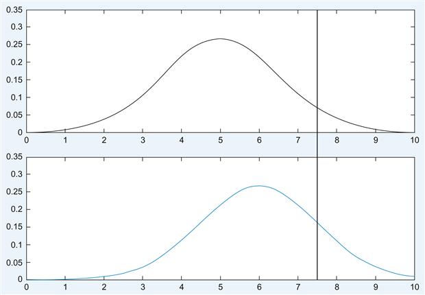
Back to SDT. If you did everything right, you can now cast the problem in terms of signal detection theory. It should look something like Figure 10.1.
The plot in Figure 10.1 contrasts the case of stimulus absence versus stimulus presence; firing rate in impulses per second is plotted on the x-axis, whereas probability or frequency is plotted on the y-axis. The thick vertical black line represents the criterion level we chose.
The upper panel represents the case of an absent stimulus. For the cases to the right of the black line, the neuron concluded “stimulus present,” even in the absence of a stimulus. Hence, they are false alarms. Cases to the left of the black line are correct rejections. As you can see, at a criterion level of 7.5 impulses per second, the majority of the cases are correct rejections.
The lower panel represents the case of a present stimulus. For the cases to the left of the black line, the neuron concluded “stimulus absent,” even in the presence of a stimulus. Hence, they are misses. Cases to the right of the black line represent hits. At a criterion level of 7.5 impulses per second, the majority of the cases are misses.
We are now in a position to discuss and calculate the receiver operating characteristic (ROC) curve for this situation, defined by the difference in mean firing rate, variance, and shape of the distribution. The exotic-sounding term receiver operating characteristic originated in engineering, in particular the study of radar signals and their interpretation.
Generally speaking, an ROC curve is a plot of the false alarms (undesirable) against hits (desirable), for a range of criterion levels. “Area under the ROC curve” is a metric of how sensitive an observer is, as will be discussed later. Given the conditions that you can generally assume, ROC curves are always monotonically non-decreasing curves. In the context of tests, you plot the hit rate (or true positive rate or sensitivity) versus the false positive rate (or 1-specificity) to construct the ROC curve. Keep this in mind for future reference. It will be important.
First, try to plot the ROC curve:
for ii = 1:1:length(y) %Going through all elements of y
FA(ii) = sum(y(1,ii:length(y))); %Summing from ith element to rest → FA(ii)
HIT(ii) = sum(z(1,ii:length(y))); %Summing from ith element to rest → Hit(ii)
FA = FA./100; %Converting it to a rate
HIT = HIT./100; %Converting it to a rate
Note: This code could have been written in much more concise and elegant ways, but it is easier to figure out what is going on in this form.
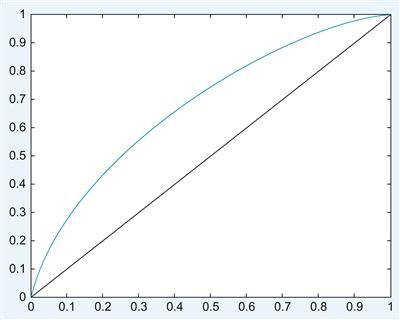
To get the ROC curve, see Figure 10.2.
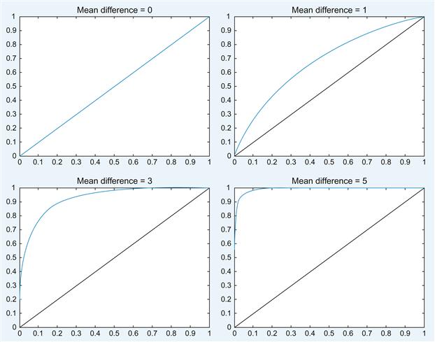
Note that the false alarms and hits are divided by 100 to get a false alarm and hit rate. The black line represents a situation in which hits and false alarms rise at the same rate – no sensitivity is gained at any point. As you can see, this neuron is slightly more sensitive than that, as evidenced by the deviation of its ROC curve from the black identity line. However, it rises rather gently. There is no obvious point where one should set the criterion to get substantially more hits than false alarms. This is largely due to the small difference in means between the distributions, which is smaller than the variance of the individual distribution. By experimenting with different mean differences, you can explore their effect on the ROC curves.
It becomes readily apparent that the ability to choose a criterion level that allows you to give a high hit rate without also getting a high false alarm rate is dependent on the difference between the means of the distributions. The larger the difference (relative to the variance) between the means, the easier it is to set a reasonable criterion level. For example, a mean difference of 5 allows you to get a hit rate of 0.9 virtually without any false alarms. This also gives a normative prescription to reduce false alarms: If you want to reduce false alarms, you should increase the difference in the means of the measured parameter between conditions of signal present (e.g., a fire) and signal not present (e.g., no fire). The clearer the parameters you choose to differentiate between these two cases, the better off you will be. A similar case can be made for the variance of the signals. The less variance (often noise) there is in the signals, the better off you will be, when you are trying to distinguish between them. Hence, in order to create highly sensitive tests that discriminate between two situations, one needs to measure parameters that can be measured reliably without much noise but which exhibit a large difference in the mean parameter value, given the different situations in question.
The concept of difference (or distance) between means relative to the variance is of central importance to signal detection theory. Hence, it received its own name: Discriminability index (d′ or d prime). d′ is defined as the distance between the means of the two distributions normalized (divided) by the joint standard deviation of the two distributions. Conceptually, it is an extension of the signal to noise ratio (SNR)—from means to mean differences. Here, it can be interpreted as a representation of signal strength relative to noise.
Importantly, d′ determines where an optimal criterion level should be set. For example, if d′ is very high, you can get 100% hits without any false alarms, by setting the criterion level properly. The situation is slightly more complicated when d′ is small, but there is a prescriptive solution for this case as well—it is discussed below.
This point makes intuitive sense. The errors derive from the fact that the “signal-present” and “signal-absent” distributions overlap. The more they overlap, the higher the potential for confusion. If the distributions don’t overlap at all, you can easily draw a boundary without incurring errors or making mistakes.
So far, so good. One central concept of signal detection theory that we are still missing is the notion of a likelihood ratio, or rather the use of likelihood ratios in signal detection theory.
While they sound rather intimidating, likelihood ratios are extremely useful because they are abstract enough to be powerful and flexible, yet specific enough to be of practical use. Hence, they are used in many fields, particularly diagnostics, but more generally in almost all of science. If you want to grasp the core of the concept, it is important to first strip off all these uses—some of which you might be already familiar with—and understand that it originally comes from statistics, or rather probability theory.
If you happen to appreciate analytical statistics, you might be appalled by the purely intuitive treatment of the likelihood ratio in this chapter. However, we deem this treatment appropriate for the purposes of our discussion.
Consider a situation in which you throw a fair and unbiased six-sided die. Each side has a probability of 1/6, which is about 0.1667. In other words, you expect the long-term frequency of a particular side to be 1 in 6. If you now want to know the probability that the die is showing one of the three lower numbers, you add the three individual probabilities and arrive at 0.5. Similarly, the probability that the die will show one of the three higher numbers is equally 0.5.
In other words, the ratio of the probabilities is 0.5/0.5=1.
If you ask what the probability ratio of the upper 4 versus the lower 2 numbers is, you arrive at (4*0.1667)/(2*0.1667)=0.666/0.333=2/1=2. In other words, the ratio of the probabilities is 2 and—in principle—you could call this a likelihood ratio.
In practice, however, the term likelihood ratio has a specific meaning, which we will briefly develop here.
To do so, we have to do some card counting. Let’s say a deck of cards contains eight cards valued 2 to 9. In each round, the dealer draws two cards from this deck (without showing them to you). There is an additional, special deck that contains only two cards: one that is valued 1 and one that is valued 10. In the same round, the dealer draws one card from this special deck—again without showing it to you. However, the dealer does inform you of the total point value of all three cards on the table. Your task is to guess whether the card from the special deck is a 1 or a 10.
While this may sound like a rather complicated affair, the odds are actually hugely in favor of the player once you do an analysis of the likelihood ratios. So don’t expect to see this game offered in Vegas any time soon.
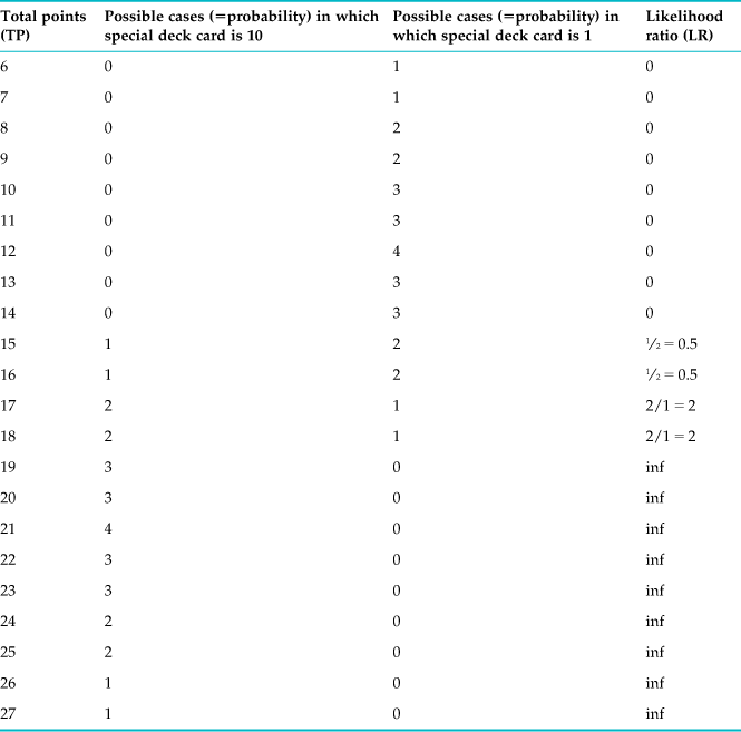
Instead, let us analyze this game—we happen to call it Chittagong—for educational purposes. The highest possible point value in the game is 27, and it can happen only if you get the 10 in the special deck and the 8 and 9 in the normal deck. So there is only one way to arrive at this value. Similarly, the lowest possible point value is 6—by getting 1 in the special deck as well as 2 and 3 in the normal deck. This case is also unique. Everything else falls somewhere in between. So let us construct a table where we explore these possibilities (see Table 10.3).
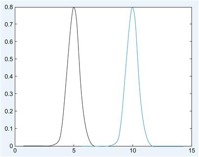
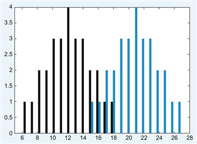
You can immediately see that vast regions of the table are not even in play. If the total value is below 15, you know that the special card had to be a 1. Moreover, if the total value is above 18, you know that the special card had to be a 10. Only four values are up to guessing, and even here, the odds are very good: As the player, you should guess 1 for 15 and 16, but 10 for 17 and 18. This state of affairs is due to the large difference between 1 and 10, relative to the possible range of normal values (5 to 17). In other words, d′ is very high in this game. This becomes immediately obvious when you plot the frequency distribution as histograms (10=blue, 1=black), as shown in Figure 10.5. This figure should look vaguely familiar (compare it to Figure 6.4).
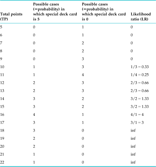
Reducing the mean difference by 4 does change the distance between the distribution as well as the overall range. Suppose the cards in the special deck are replaced with two cards worth 0 and 5 points, respectively. What does the histogram of the frequency distributions look like now? (See Figure 10.6.)
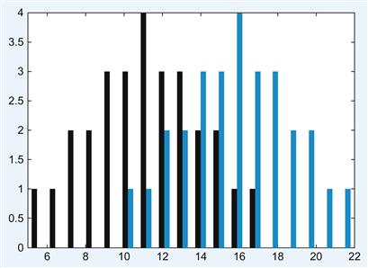
Figure 10.6 Histogram of frequency distribution with a smaller mean differences between the special cards (0=black, 5=blue).
The table of likelihood ratios, shown in Table 10.4, reflects this change.
As you can see, there is an intuitive and clear connection between likelihood ratio and d′. Of course, this relationship has been worked out formally. We will forgo the derivation here in the interest of getting back to neuroscience.
In this simple case, you can just set the criterion at the ratio between the probabilities. If this ratio is smaller than 1, guess 0. If it is larger, guess 5.
In the technical literature, the likelihood ratio takes more factors into account: the prior probability as well as payoff consequences. Let us illustrate this case. Suppose there are not 2, but 10 cards in the special deck: You know that 9 have a value of 5, 1 has a value of 0. Hence, there is an a priori chance of 9/10 that the card will have a value of 5, and this does influence the likelihood ratio, as it should. Taking payoff consequences into account makes good sense because not all outcomes are equally good or bad (see the discussion at the beginning of the chapter). A casino could still make money off this game by adjusting the payoff matrix. For example, it could make the wins very small (as they are expected to happen often in a game like this), but the rare losses could be adjusted such that they are rather costly. A player has to take these considerations into account when playing the game and setting an optimal criterion value.
To make this point more explicit, the likelihood ratio can be defined as follows:
 (10.1)
So the likelihood ratio of an event e is the ratio of two conditional probabilities. One is the probability of the event given state si; the other, the probability of the event given state sj. lij is always a single real number.
Moreover, we already discussed a more general situation where the likelihood ratio takes prior probabilities and payoffs into account:
 (10.2)
This is particularly important for real life situations, where not all outcomes are equally valuable or costly.
As we alluded to before, the likelihood ratio is closely linked to ROC curves. Specifically, it is very important to characterize optimal behavior.
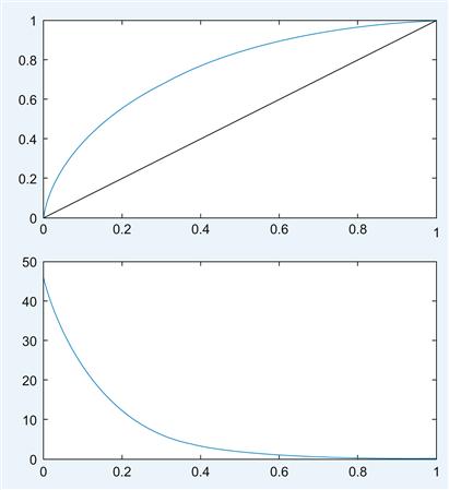
These considerations influence the likelihood ratio at which you should set your decision criterion. Importantly, there is a direct relationship between likelihood ratio and ROC curve: The slope of the ROC curve at a given point corresponds to the likelihood ratio criterion which generated the point (Green and Swets, 1966). In other words, an inspection of the slope can reveal where the criterion should optimally be set.
Let us illustrate these claims by revisiting the distributions introduced at the beginning of the chapter.
Use this code to plot the slope of the curves, analogous to Figure 10.2.
%Note that x is ordered. If you start with empirical data, you will have to sort them %first.
FA(ii) = sum(y(1,ii:length(y)));
HIT(ii) = sum(z(1,ii:length(y)));
plot(baseline,baseline,’color’,’k’)
m1(ii) = FA(ii)-FA(ii+1); %This recalls the
The slope of the ROC curve is plotted in the lower panel; see Figure 10.7.
The philosophical implications of signal detection theory are deep. The message is that—due to the stochastic structure of the real world—infallibility is, in principle, impossible in most cases. In essence, in the presence of uncertainty (read: in all real life situations), errors are to be expected and cannot be avoided entirely. However, signal detection theory provides a precise analytical framework for optimal decision making in the face of uncertainty, while also being able to take into account subjective value judgments (such as preferring one kind of error over another).
As you might have noticed, we are really only scratching the surface here. Because situations in which a signal detection theory perspective is useful are truly ubiquitous—think of any kind of selection and quality control process, such as hiring decisions, admission decisions, marriage, dating, to say nothing of the myriad applications in materials science—signal detection theory has become a bottomless well. This should not be surprising, as it is arguably at the very heart of cognition itself. Yet, this led to a situation in which even specialists can be overwhelmed by the intricacies of the field. Hence, the point of this brief treatment was to cover the conceptual essentials and their application. We are confident that it is enough to get you started in applying signal detection theory with MATLAB to problems in neuroscience.
For further reading, we highly recommend the classical and elaborate Signal Detection Theory and Psychophysics by Green and Swets (1966); the latest edition is still available in print. It nicely highlights the role of signal detection theory in modern cognitive science with many colorful examples.
10.4 Project
The project for this chapter is very straightforward. Many uses of signal detection in neuroscience involve the measurement of some “internal response” in addition to measuring a behavioral response (e.g., deciding whether a stimulus under the control of the experimenter is present or not). We assume that you do not currently have access to measure a “deep” internal response, such as firing rate of certain neurons that are presumably involved in the task. Instead, we ask you to redo the experiment in Chapter 8, but with a twist. Instead of just asking whether a faint stimulus is present or not, now elicit 2 judgments per trial: One whether the stimulus is present or not, the other how confident the observer is that it was present or not, on a scale from 1 (not certain at all) to 9 (very certain). Replot the data in terms of certainty. Get two distributions of certainty (one for situations where the stimulus was present, the other where it was not present). After doing so, please answer and explore the following questions:
Where does the internal criterion of the observer lie?
What is the d′ of the certainty distributions?
Construct the ROC curve for the data (including slope).
How sensitive is the observer? (Compare the area under the ROC curve with the area under the diagonal reference curve.)
Can you increase d′ by showing a different kind of stimulus?
Can you shift the position of the criterion by biasing the payoff matrix for your observer (e.g., rewarding the observer for hits)?
