SEVEN
Neighborhood Segregation by Class and Race
Some of the most obvious and enduring features of the American metropolitan landscape are the stark differences in who lives where. The residential populations inhabiting a neighborhood typically consist of one predominant racial or ethnic group (“race” hereafter) and represent a narrow range of incomes and wealth (“class” hereafter). This homogeneity, as viewed within neighborhoods, translates into a geographic pattern of segregation when viewed among neighborhoods. As I will demonstrate in chapters 8 and 9, this segregation by race and class is as pernicious in its impact as it is clear-cut in its existence. My first purpose here is to document the status of neighborhood segregation by race and class, and to explain how neighborhoods transition from occupancy primarily by one group into occupancy by another. Second, I aim to develop a conceptual model of metropolitan structures and causal forces within which one can perceive the causes of neighborhood segregation by race and class holistically.
At the outset, it is useful once more to consider this topic from the perspective of adding more realism to my Housing Submarket Model of neighborhood change. In this chapter, I relax the prior assumptions that (1) preferences for the neighborhood population components of housing quality are homogeneous among households; (2) housing search outcomes are race neutral; (3) willingness and ability to pay for housing can always be freely exercised, subject to information constraints; and (4) suppliers of housing can develop wherever in whichever quality submarket category they find most profitable. As for the first point, the current neighborhood racial, ethnic, and income group composition is potentially assessed as “quality” differently, depending on the race, ethnicity, and income of the particular household. Thus, sorting within a generically defined housing quality submarket may occur by those seeking more homogeneity of households occupying the housing stock in the neighborhood in question. As for the second and third points, here I allow for the possibility of illegal discriminatory acts constraining the housing and neighborhood options available to minority home seekers. Finally, I will consider the role of local governments in limiting via land-use regulations the types and qualities of dwellings that can be developed within the jurisdiction, thereby producing more homogeneous spatial clusters of submarkets, and ultimately income groups, than would have been produced by an unfettered market.
Segregation by Class and Race: Trends and the Current Situation
Segregation by Class
National trends in rising inequality in household income and wealth, which academic work and the popular press have documented well, are mirrored by increases in the degree to which households in different income groups live apart from each other.1 No matter how economic segregation is measured, trends show dramatic if uneven growth in the degree of segregation by income since the 1970s.2 Sean Reardon and Kendra Bischoff, for example, used the proportion of families living in neighborhoods that have median income at least 50 percent above the metropolitan area median income (“extremely affluent”) or 50 percent below area median income (“extremely poor”) to reveal changes in the degree to which American families are residing in communities stratified by economic status.3 They found that in 2012, 34 percent of American families lived in neighborhoods that were either extremely affluent or extremely poor, a rate that is more than double the 15 percent rate observed in 1970.4 The magnitude of income disparity between neighborhoods is substantial, even when not considering the income group extremes. To illustrate, Stuart Rosenthal and Stephen Ross showed that the median income of neighborhoods in the 75th percentile of the national metropolitan neighborhood distribution was 55 percent more than the median income of neighborhoods in the 25th percentile.5
Despite the overall upward trend in neighborhood segregation by income, there remains considerable diversity of incomes in the average American neighborhood, though less so at the extremes noted above. With colleagues Jason Booza and Jackie Cutsinger, I probed the economic composition of metropolitan neighborhoods in 2000, categorized by various median income ranges.6 In very low-income neighborhoods (that is, those with median incomes below 50 percent of the area’s median income), 59 percent of the residents had incomes below 50 percent of the area median, 19 percent were between 50 and 80 percent of the area median, 8 percent were between 80 and 100 percent of the area median, and only 14 percent earned more than the area median income. At the other extreme, in very high-income neighborhoods (that is, those with median incomes above 150 percent of the area’s median income), 62 percent of the residents had incomes above 150 percent of the area median, 11 percent were between 120 and 150 percent of the area median, 7 percent were between 100 and 120 percent of the area median, and only 20 percent earned less than the area median income. In moderate-income neighborhoods (that is, those with median incomes between 80 and 100 percent of the area’s median income) there was considerably more diversity: each of the six income groups specified by US Department of Housing and Urban Development guidelines comprised at least 12 percent of the population, and none exceeded 22 percent. We also identified a rapidly growing phenomena we called “bipolar neighborhoods:” those whose populations are jointly dominated by families earning less than 50 percent and those earning more than 150 percent of the area’s median income.7 At the same time, we also highlighted a distinctive reduction in neighborhoods having the greatest diversity of income groups: those with median incomes in the middle ranges.8
Although the growth of more homogeneously affluent neighborhoods is an important contributor to the rise of economic segregation,9 most of the public concern about the issue stems from the rise of spatially concentrated disadvantage. Paul Jargowsky documented trends in the proportion of Americans living in neighborhoods with a poverty rate of 40 percent or greater in a series of reports. He demonstrated that there was substantial growth in concentrated poverty from 1970 to 1990, a decline of such neighborhoods during the prosperous 1990s, but then a substantial rebound in concentrated poverty since 2000, due largely to the Great Recession.10 Since 2000, the number of extreme poverty neighborhoods swelled by more than 75 percent and the number of Americans living in such neighborhoods rose from 7.2 million to 13.8 million people, a remarkable increase of more than 90 percent.11
Neighborhood Class Transitions
A related important issue is the degree to which patterns of neighborhood income segregation are stable over time across geography. That is, does the economic profile of a neighborhood typically remain constant over long periods, or are upward and downward income succession common? The answer depends on how one measures neighborhood economic status and its change, and what period and which type of neighborhood one considers.12 The general pattern is that there is considerable flux in neighborhood status, though there is more stability at both extremes of neighborhood affluence and disadvantage, however measured. How much flux there will be varies according to the decade, the metropolitan scale, and the overall economic circumstances in the particular metropolitan area during that decade.
Looking across all metropolitan neighborhoods from 1970 to 2000, Stuart Rosenthal found the greatest stability among neighborhoods with less than 15 percent poverty rates, on average: 81 percent of them in that category in 1970 remained in the same category by 2000.13 Among neighborhoods with over 45 percent poverty, 43 percent remained in the same category between 1970 and 2000. Those with intermediate levels of poverty were less stable: roughly 60 percent of these neighborhoods failed to retain their 1970 absolute poverty status by 2000. Analyses of Los Angeles County neighborhoods by Robert Sampson, Jared Schachner, and Robert Mare suggest that relative stability at the extremes is contingent upon metrowide economic conditions. During the 1990 to 2000 period, 97 percent of neighborhoods in the poorest quintile measured by median income remained in that category, but from 2000 to 2010 only 68 percent of these neighborhoods remained in this category. The comparable figures for neighborhoods starting in the richest quintile were 70 percent and 87 percent.14 Using changes in finite categories of income understates the variability of neighborhood status over time, however, especially in the extreme poverty categories. With colleagues Roberto Quercia, Alvaro Cortes, and Ron Malega, I employed absolute decadal changes of five percentage points or more in the poverty rate to identify a change in neighborhood status. By this measure, we found that roughly equal thirds of neighborhoods that had 40 percent or higher poverty rates remained stable, experienced upward succession, or experienced downward succession during the ensuing decade.15
Stuart Rosenthal has taken the longest-term view of this topic, analyzing neighborhood changes over half a century across thirty-five metropolitan areas.16 He concluded that change is the norm over this period: on average, a neighborhood changed its median income (relative to the full sample) by 12 to 15 percent in absolute value per decade from 1950 to 2000. Remaining in the same relative median income quartile was still more common at the extremes, however. Thirty-four percent of neighborhoods in the lowest income quartile and 44 percent of those in the highest income quartile in 1950 remained so in 2000; the contrasting figures for the middle two quartiles were only 26 to 27 percent. Of those neighborhoods substantially changing their relative position, most neighborhoods in the lower half of the income distribution tended to move up in status, while most neighborhoods in the upper half tended to move down.17
Perhaps the highest-profile type of neighborhood class transition is termed “gentrification”: a process by which many households of greater socioeconomic status move into neighborhoods occupied predominantly by lower-income households.18 Though scholars have employed the term gentrification in different ways, Ingrid Ellen and Lei Ding provide an appealing formulation that provides a clear portrait of the significance of this phenomenon in US metropolitan areas over the last three decades.19 They examine the degree to which low-income central-city neighborhoods (census tracts having median household incomes placing them below the 40th percentile of their metropolitan area’s neighborhood income distribution) have exhibited substantial increases in their neighborhood’s standing relative to that of their metropolitan area (that is, an increase in the ratio of the neighborhood mean to the metropolitan mean of the particular indicator by more than ten percentage points) during a decade. During the 1980s, about 9 percent of these neighborhoods experienced such a substantial increase in their relative median incomes; during the 1990s and 2000s this figure rose to 14 percent. Changes appear even more prevalent when measured by shares of college-educated people. During the 1980s, about 27 percent of low-income neighborhoods saw their relative share of college-educated residents rise substantially; this dropped slightly to 25 percent during the 1990s, but rose to 35 percent during the 2000s.
Beyond describing the frequencies of various types of neighborhood class transitions, several researchers have probed the predictors of such changes using sophisticated multivariate models. Stuart Rosenthal showed that the older the housing stock in a neighborhood, and the more that stock represented subsidized housing, the greater its chances of experiencing a decline in its economic status.20 Several analyses of patterns from the 1970s and 1980s indicated that higher percentages of black residents predicted subsequent declines in the average income levels of the neighborhood, though this relationship may have reversed itself more recently; moreover, the relationship appears not to be the same for Hispanic neighborhood composition.21 More home foreclosures and higher percentages of renter-occupied dwellings also are predictive of the declining economic status of neighborhoods.22
Segregation by Race
Economic inequality across American neighborhoods often overlaps with racial and ethnic inequality.23 According to a variety of commonly used measures,24 the residential segregation of blacks and non-Hispanic whites continues to be extremely high in many metropolitan areas, although black/white segregation has declined steadily since 1970.25 The average metropolitan black household in 2010 lived in a neighborhood that was 41 percent black and 40 percent white. Measures of evenness in the spatial distribution of both Hispanics and Asians relative to whites show, on the contrary, slight increases in segregation over time, though they still do not approach the geographic dissimilarity of blacks and whites in most areas. The residential isolation of Hispanics and Asians also has increased over time, consistent with the rapid population growth of both groups. The average metropolitan Hispanic household in 2010 lived in a neighborhood that was 42 percent Hispanic and 40 percent white; the comparable figures for Asians were 18 and 52 percent.26
As stark as these figures are, they are even more dramatic for children, who are more residentially segregated by race than adults are. Ann Owens has documented that, in the one hundred largest metropolitan areas in 2010, the average black child lived in a neighborhood where only 22 percent of children were white and over half were black, whereas the average black adult lived in one where 33 percent of adults were white and only 46 percent were black.27 The average Hispanic child lived in a neighborhood where 55 percent of children were Hispanic and 25 percent were white; the average Hispanic adult lived in one where 45 percent of adults were Hispanic and 35 percent were white.
Neighborhood Racial Transitions
Though it is clear that American neighborhoods’ racial compositions typically are not representative of their corresponding metropolitan area’s composition, there certainly are examples of diverse neighborhoods. In an encouraging trend, they appear to be both growing in number and becoming more stable in their diversity over time. Ingrid Ellen, Keren Horn, and Katherine O’Regan examined metropolitan neighborhoods from 1990 to 2010 and found that the share they considered integrated (that is, those in which the group in the minority comprised at least 20 percent of the population) rose from slightly less than 20 percent to slightly more than 30 percent during this twenty-year period.28 This increase was due to both a small increase in the number of neighborhoods becoming integrated for the first time and a more sizable increase in the share of integrated neighborhoods that remained so during the period. Indeed, stability of integration was the hallmark: between 1990 and 2000, 77 percent of integrated neighborhoods remained so; from 2000 to 2010, this percentage rose to 82 percent. Neighborhoods that experienced a larger growth of minority residents during the prior decade, were located closer to areas of minority concentration, and had more homeowners with children were less likely to remain stably integrated.29
The typical residential mobility dynamic fueling integration was minority households moving into neighborhoods predominantly occupied by whites. The predominantly white-occupied neighborhoods that ultimately became more integrated began the decade with slightly lower percentages of white residents, homeownership rates, and median incomes, and were somewhat closer to minority-dominated areas. Ellen, Horn, and O’Regan also showed that white in-migration was most likely to be the force integrating lower-income, primarily renter-occupied, center-city minority neighborhoods. This latter mobility pattern appears to be rapidly accelerating. Ellen and Ding demonstrated that in recent decades a growing number of low-income central-city (predominantly minority-occupied) neighborhoods witnessed large increases (i.e., more than ten percentage points) in their percentages of white residents relative to their metropolitan area’s percentage.30 During the 1980s, only about 5 percent of such low-income minority neighborhoods saw their relative share of white residents rise substantially; this rose slightly to 7 percent during the 1990s, but jumped to 16 percent during the 2000s.
The Dynamics of Neighborhood Change by Class and Race
The foregoing descriptive portrait of neighborhood class and race profiles makes it clear that, while segregation is the norm in aggregate, many individual neighborhoods experience considerable flux in the composition of their populations. Why this process of neighborhood population change occurs and why it sometimes yields a wholesale replacement of one group by another instead of a stable mix has been the subject of considerable investigation. On the one hand, the process of neighborhood class or racial change is deceptively simple: if the composition of the in-movers does not match the composition of the out-movers, the neighborhood’s aggregate composition must change. What makes this process fascinating is that the aggregate composition of the neighborhood will partly influence the composition of both in- and out-movers. Thus, these flows of people are endogenous because people react to neighborhood composition and, by doing so, change it. The fact that the groups competing for housing in the neighborhood many not similarly value its aggregate class or racial composition is the reason why a mixture of groups may not prove stable. In this section, I present a simple model of the neighborhood transition process that makes these points clear and demonstrates their import.31
To understand why neighborhoods change their population composition, one must focus fundamentally on who is moving in, instead of who is moving out.32 A simple thought experiment suffices to make this vital point. Imagine some hypothetical neighborhood, with a mix of groups X and Y currently in residence. Now if only members of group X were to occupy every vacancy opening up in the neighborhood for the indefinite future, the neighborhood must inevitably change to represent a greater and greater share of X residents, so long as some vacancies are generated by members of group Y. The rate at which the neighborhood will change its composition will be influenced by whether the in-flow and out-flow profiles match, but its ultimate fate will not. It follows, then, that one must ultimately base a model of neighborhood population transition on which group(s) will most likely comprise the stream of in-movers.
The Willingness to Pay Model offers a simple but powerful way to accomplish this.33 In simplest form, it assumes that two distinct class or race groups are competing for housing in a particular hypothetical neighborhood containing housing of a homogeneous quality. Purchasing power and preferences for housing and the residential composition of the neighborhood are assumed to be homogeneous within, but not across, both groups. In a world of perfect information and no discrimination, any housing vacancy in this neighborhood will be allocated to any member of the group who is willing to pay more.34 Each member of the homogeneous group may be thought of as having an implicit “willingness to pay” function that indicates how much the household is willing and able to pay to occupy a vacant dwelling in the neighborhood in question, for each alternative class or race composition of that neighborhood. The variations in willingness to pay across these alternative compositions are a manifestation of the common preferences among households in the group: they will manifest greater willingness to pay for the preferred compositions in direct relation to the strength of this preference. Holding constant for the moment the neighborhood composition, the aggregate supply-and-demand characteristics present in the housing quality submarket represented in the hypothetical neighborhood will influence the amount that a typical member of the particular group is willing to pay. If, for example, the group’s population has been growing rapidly and the target submarket in question has been inelastic in its response across the metropolitan region, the level of willingness to pay for any such vacant dwellings in this neighborhood will ratchet upward.
A graphic exposition of the Willingness to Pay Model demonstrates the insights it provides for explaining neighborhood change and the tenuousness of diverse populations in neighborhoods. Start with a hypothetical neighborhood containing housing of a homogeneous quality, which remains so throughout this illustration. The two household groups competing for this neighborhood are X and Y. I show the possible combinations of these two groups residing in the neighborhood along the horizontal axis of figure 7.1; the willingness to pay is measured on the vertical axis. Assume that all members of group X prefer “modest integration:” 20 percent Y and 80 percent X neighbors, with marginally less desire to have ever greater or ever smaller percentages of their own group as neighbors. By contrast, assume that all members of group Y are indifferent to the race or class composition of their neighbors: X and Y neighbors are perfect substitutes. These last two assumptions imply that members of X will be willing to pay the most if the neighborhood exhibits 80 percent of X, but there is no variation in the willingness to pay by members of Y regardless of the neighborhood’s composition.
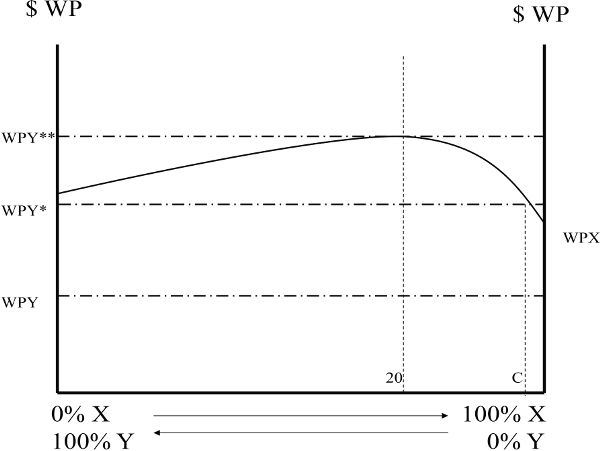
Figure 7.1. The Willingness to Pay Model of neighborhood composition, and its stability. Source: author’s adaptation based on Schnare and MacRae 1978; Colwell 1991; and Card, Mas, and Rothstein 2008.
Suppose that group X was initially the sole occupier of the neighborhood. In this situation, there may be little competition from group Y because perhaps they are few in number in the region, have insufficient incomes to consider bidding for housing in the neighborhood, or happily occupy housing elsewhere. In this initial circumstance, whenever a vacancy appears, the higher bidder will emerge from group X because its willingness-to-pay function (shown as WPX in figure 7.1) dominates that of group Y (shown as WPY). The in-movers will all be members of group X indefinitely, and the neighborhood composition will remain homogeneously X.
Now suppose that time has passed, and the circumstances of group Y have changed such that they have intensified their competition for this neighborhood, embodied in WPY*. In this case, a vacancy occurring in the all-X neighborhood will be filled by a member of group Y, since WPY* is greater than WPX at 100 percent X. Y will also fill the next vacancy, and so on, until the neighborhood eventually assumes a mixture of C percent X and 100 – C percent Y residents. If the aggregate personal circumstances, demographic and economic conditions, and housing market context shaping both WP functions remain constant, the neighborhood will remain stably mixed at this composition indefinitely. Both X and Y have equal odds of winning the competition for any vacancy occurring in a neighborhood with C percent X population. Should the in-mover randomly turn out to be a member of group X, the neighborhood percentage of X will exceed C and a member of group Y thus will win the bid for the next vacancy, restoring stability at C. The opposite will occur should the in-mover be a member of group Y. However, should the level of WPY continue to rise, the neighborhood’s share of Y will as well. Eventually this share will reach 20 percent with WPY**, the threshold of instability (that is, the tipping point) in this particular case. Any further shifts upward in WPY will mean that the neighborhood will tip inexorably to occupancy solely by group Y members, as they will continue to outbid group X for any future vacancies, regardless of its composition.35
Despite its many simplifying assumptions, the Willingness to Pay Model illuminates several realistic generalizations regarding the prospects for stable diversity of groups in neighborhoods. The chances of a substantial diversity of groups in a particular neighborhood remaining stable over time will be enhanced the degree to which one or more of the groups manifest certain characteristics. These include (1) being unwilling to pay substantially more for larger shares of their own group, (2) being willing to pay substantially more for diverse neighborhoods instead of those where one group predominates, (3) not rapidly changing the number of households competing for the housing submarket(s) predominant in the particular neighborhood, and (4) not being systematically underrepresented in the bidding process for dwellings in the neighborhood due to spatial biases (discussed in chapter 5) or illegal discriminatory barriers.
There have been numerous attempts over the last half century to develop conceptual and simulation models trying to explain how segregation of groups can be an equilibrium outcome of an unfettered housing market allocation process driven only by preferences for composition of the neighborhood.36 The latest generation of agent-based (cellular automata) computer models has shown how complex aggregate patterns of residential segregation can arise from a small set of simple, agent-level social dynamics operating within stylized metropolitan contexts.37 This outcome is not inevitable, however; it depends on the nature of stylized preferences specified. This has been convincingly demonstrated by Elizabeth Bruch and Robert Mare, who show that considerable segregation results when simulated individuals equally prefer all options when they are in the majority over all options where they are in the minority.38 However, when one employs alternatives involving finer gradations of preferences for own-group neighbors, much less segregation is simulated. Finally, when preference structures are simulated that match as closely as possible the range of racial preferences revealed in American public opinion surveys, virtually no segregation emerges.39
It is clear that the interactive dynamics that come into play when households are sorting themselves across metropolitan space are much more multifaceted and nuanced than simulations based on stylized preferences can simulate, or than only one aspect of this complex choice problem can explain. In what follows, I advance a conceptual model that attempts to synthesize all the primary causal forces behind neighborhood class and racial composition, and to elucidate how they are interconnected, often in mutually reinforcing ways.
A Structural Model of Neighborhood Segregation by Class and Race
When viewed independently, multiple and disparate causal forces determine residential segregation by class and segregation by race. When viewed holistically, many of these forces are the same for both types of segregation, and some are distinct but interrelated. More fundamentally, some explanatory forces are endogenous, that is, they are themselves influenced by the degree of segregation extant in the metropolitan area, and the two forms of segregation are themselves mutually reinforcing.40 I begin presenting this holistic model by delineating each of the proximate causes of class and racial segregation that scholars have forwarded before synthesizing them in a common framework.41 I believe that this original, holistic framing is powerful because it helps explain why both forms of segregation have been such a durable feature of American neighborhoods.42
Proximate Causes of Class Segregation
There are seven distinct proximate causes of the residential segregation of households distinguished by their economic status.43 First, households will choose locations partly based on their relative valuation of work commuting time and consumption of housing. When confronting a geographic pattern of employment clusters where the value of land per acre is bid up, households making a residential location choice must trade off commuting time with housing expense (and thus the quantity they can consume). If there are substantial differences in the ways that different income groups relatively value these two elements, they will tend to sort spatially according to proximity to employment.44 See path C in figure 7.2. Of course, this first proximate cause takes no heed of preexisting patterns of housing development, location-specific amenities and disamenities, and overlays of local political jurisdictions. I emphasize these dimensions below.
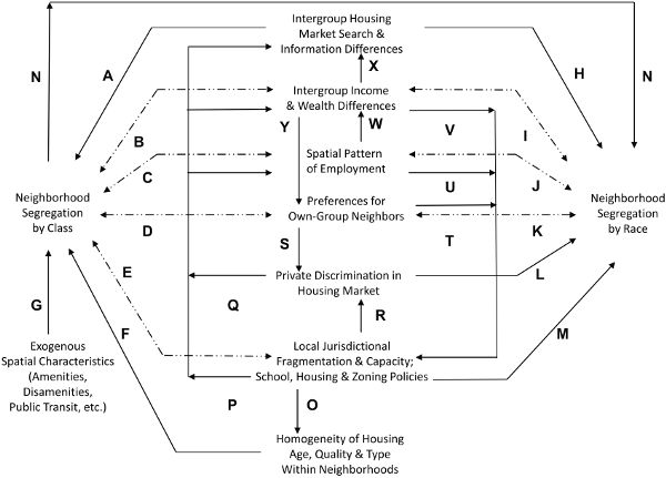
Figure 7.2. A structural model of neighborhood segregation by class and race
A second proximate cause is class sorting according to the age of housing stock, a position advanced by Jan Brueckner and Stuart Rosenthal. Assuming that, all else being equal, older housing is generally of lower quality (smaller size, obsolete systems and amenities, health and safety hazards, poorer upkeep, etc.) and is more expensive to maintain at a constant quality, higher income groups will outbid lower-income groups for locations with newer dwellings. Inasmuch as housing typically has been built in a consistent temporal pattern from a city’s historic core outward, such newer dwellings are more likely to be located nearer the fringes of the urbanized area. The exception is core redevelopment areas that might have witnessed wholesale demolition or rehabilitation of older housing.45 See path F in figure 7.2.
The third proximate cause is that different classes of households will have different willingness to pay for a wide variety of natural and human-made attributes that vary geographically, often in idiosyncratic ways, across any particular metropolitan area, These attributes are predetermined in the sense that which groups ultimately live near them exert no influence over them. Natural amenities such as scenic waterfronts and desirable topographical features, and human-made attractions such as parks and concentrations of historically significant architecture may serve as magnets for upper-income settlement because of the greater income elasticity of demand for such luxuries.46 Conversely, areas characterized by undistinguished natural features, few public amenities, and heavy concentrations of pollution will be avoided by higher-income groups, and will be left as residual spaces to households that can only afford the cheapest accommodation.47 Locations close to public transportation links are also relevant here, though it is less clear whether this amenity is relatively more attractive to the rich who place a higher value on their time, or the poor who may not own a vehicle.48 See path G in figure 7.2.
The fourth proximate cause is amenities and disamenities associated with neighborhoods that arise endogenously as particular households occupy them.49 Households with homophily preferences will be more willing to pay to live in neighborhoods where their own income group is dominant than in otherwise identical neighborhoods where their group is underrepresented, and they will make intraurban mobility choices accordingly.50 Related preferences to have appropriate peer groups for their children may drive upper-income parents to cluster with parents of similar class status in the same neighborhoods and schools.51 If lower-income groups are thought to generate negative externalities (such as crime) in the neighborhood, thereby eroding the quality of life and perhaps encouraging socially problematic behaviors by other residents—topics that I will explore in detail in chapter 8—higher-income households will try to avoid neighborhoods where they live in noticeable concentrations.52 See path D in figure 7.2.
The fifth proximate cause relates to the fragmentation of most US metropolitan areas into many local political jurisdictions such as municipalities, townships, and school districts. To the extent that different classes possess different preferences about how much they are willing to be taxed for locally supplied public services and facilities and the particular composition of those services and facilities, Charles Tiebout has argued that groups will sort across jurisdictions according to the intensity and variety of tax/service package offered.53 This may be especially important for parents of school-age children who are concerned about peer effects.54 The greater the number of such jurisdictional variations, the greater the intrajurisdictional class homogeneity and the greater the segregation of classes across metropolitan space.55 Other local policies related to schools, such as whether to merge districts, develop magnet schools, or permit enrollment across district lines, may also contribute to class segregation by strengthening or weakening the link between neighborhood and school economic composition. See path E in figure 7.2.
The sixth proximate cause is that the existing housing stock in any particular neighborhood is typically quite homogenous in quality (in the broadest sense of quality that I began employing in chapter 3). This homogeneity arises because of location-specific differences in the feasibility and costs of building certain types of housing (such as the availability of bedrock to support high-rise construction), economies of scale in the development of homogeneous subdivisions, and geographic niche specializations of builder-developers.56 Due to interclass differences in the willingness and ability to pay for different housing quality submarkets (as explained in chapter 3), one would expect that if a neighborhood is dominated by a dwelling stock comprised of only one quality submarket, it will be occupied by a narrow range of income groups. In a special case, large-scale developments of public or other subsidized housing complexes can create spatial dwelling homogeneity occupied only by households within a limited range of incomes because of income-eligibility limits.57 See path F in figure 7.2.
The last proximate cause is spatial biases in housing market information, which I discussed in length in chapter 5. These biases imply that, once established in a particular geographic pattern, income groups will tend to move between dwellings and neighborhoods in ways that perpetuate current residential patterns of segregation. See path A in figure 7.2.
Of course, all the prior discussions have assumed that there is a nontrivial degree of variability in economic wherewithal among households in the metropolitan area. Obviously, the degree of income and wealth inequality among households is neither constant across metropolitan areas, nor is it constant over time within a metropolitan area. The greater inequality among classes, the more powerful all the above forces are likely to be in producing residential segregation. See path B in figure 7.2.
Proximate Causes of Racial Segregation
There are six proximate causes of racial segregation; five are closely related to their counterpart causes discussed in the context of class segregation.58 Indeed, the first is class segregation itself. Because of residential segregation by income groups (regardless of its causes) and distinctive interracial differences in the distribution of income and wealth, class segregation will produce de facto racial segregation.59 See paths N and I in combination in figure 7.2.
The second proximate cause of racial segregation is interracial differences in the spatial distribution of employment. If, for the moment, one takes as fixed both the location of jobs within a metropolitan area and the particular individuals comprising the work force at each such location, one can deduce that workers will tend to cluster around their respective predetermined places of employment to reduce the out-of-pocket and time costs associated with commuting. Because a much higher proportion of all minorities are employed in central cities than are whites, it follows that residential patterns should reflect this disparity, assuming that members of both races are equally averse to commuting.60 See path J in figure 7.2.
The third proximate cause is preferences for neighborhood racial composition. Both public opinion polls61 and statistical studies of willingness to pay for housing62 consistently reveal that most black and Hispanic households most prefer neighborhoods with roughly equal racial proportions, whereas whites generally prefer ones that are predominantly white-occupied. What is less clear is how and the degree to which this combination of preferences dynamically translates into segregation, as discussed at length above.63 Moreover, whites’ expressed aversion to predominantly black-occupied neighborhoods may be related to the freighted stereotypes they hold about such places, as I discussed in chapter 5. See path K in figure 7.2.
The fourth proximate cause is discriminatory acts by private housing market agents, such as property owners and real estate agents, or by private mortgage lenders. Housing market discrimination been documented at the national level in an ongoing series of matched-tester studies by Margery Austin Turner and colleagues.64 These practices can cause segregation if they serve to exclude minority home seekers from nonminority neighborhoods into which they otherwise would be willing and able to move, or if they render occurrences of neighborhood integration more transitory.65 The former set of acts includes actions such as “steering” and “exclusion”;66 the latter includes “blockbusting” and “panic peddling.”67 Indeed, it appears that minorities’ chances of encountering discrimination are much higher when they attempt to secure housing in majority white-occupied neighborhoods.68 Denial of mortgage finance (or its provision only on less favorable terms) may also hinder minorities’ ability to move into predominately owner-occupied neighborhoods that might be primarily occupied by whites.69 See path L in figure 7.2.
The fifth proximate cause is racially discriminatory acts and policies by public institutions and governmental bodies. Douglas Massey and others have documented the sordid mid-twentieth century history of segregationist policies promulgated by federal mortgage guarantors and public housing agencies.70 Explicitly discriminatory local government actions of various sorts also reinforced segregation across the country.71 Though the contemporary extent of this factor is difficult to quantify, the periodic filings of federal legal suits directed at localities’ fair housing violations suggests that this issue has not been relegated to history. Even in the absence of illegal actions, local policies related to schools, such as whether to merge districts, develop magnet schools, or permit enrollment across district lines may contribute to racial segregation by strengthening or weakening the link between neighborhood and school racial composition. See path M in figure 7.2.
The last cause of racial segregation is misinformation about housing opportunities extant in neighborhoods where few members of one’s own racial group reside.72 Due to the aforementioned spatial biases in one’s information acquisition process, minority households may have insufficient, inaccurate, and biased information about the quality of life and relative expense of housing in neighborhood inhabited primarily by whites, and vice versa.73 If their ambient level of information leads both groups to underestimate systematically the quality of life and overestimate the expensiveness of housing in the other group’s neighborhoods, they may not bother to search there for housing options. See path H in figure 7.2.
Interactions among Proximate Causes
Thus far, I have listed proximate causes of segregation as if they were independent. Clearly, they are not. Consider first the role of local jurisdictional public policies regarding affordable housing and land use zoning patterns. In the extreme, a jurisdiction may forbid any public and other forms of subsidized housing and require single-family detached homes to be built on large plots of land, thus generating a high housing cost range across the jurisdiction. Though less exclusionary than this extreme case, jurisdictions that establish large-scale zones exclusively for one particular type of housing structure will increase the homogeneity of housing values within any particular neighborhood.74 See path O in figure 7.2. Cross-locality variations in nonresidential land use zoning and business attraction policies (development fees, tax abatements, environmental regulations, etc.) will also shape the spatial pattern of employment in the metropolitan area. Interlocal differences in public service quality, especially as related to health, education, recreation, and safety, will produce differences in children’s ability to develop human capital that ultimately will contribute to intergroup income and wealth differences in the region. See path P in figure 7.2. Finally, such differences in local public service quality can promote racial discrimination because real estate agents can use such invidious distinctions as a basis for steering white home seekers away from racially diverse jurisdictions by using the subterfuge that “they have inferior services and schools.”75 See path R in figure 7.2.
Discrimination in the housing and mortgage markets imposes direct penalties (in the form of information and money) on minorities whom it victimizes. As John Yinger has demonstrated, discrimination reduces minorities’ net benefits from searching in the housing market because it erodes the quantity and quality of information that search provides, yielding thereby an estimated annual penalty of billions of dollars in foregone consumers’ surplus.76 There will be additional financial penalties exacted from minorities when they face discriminatory terms in renting accommodations or securing mortgage credit.77 Thus, in this manner discrimination contributes to interracial disparities in both information and economics; see path Q in figure 7.2.
Preferences for neighbors predominantly of one’s own economic or racial group also influence other proximate causes. Real estate sales agents may be loath to show minority home seekers vacancies in neighborhoods where their current or prospective white customer base resides if they perceive that customer base as having strong racial prejudices that might motivate retaliation against any agents who attempt to break unwritten color lines.78 Analogously, landlords of large apartment buildings who perceive their current white tenants as willing to pay a greater premium for a homogenous clientele than prospective minority tenants will have strong economic motives to cater to their white customers’ preferences and exclude any minority renters. See path S in figure 7.2. Strong preferences for homophily on class or race grounds can stimulate the formation and preservation of fragmented local political jurisdictions, since they can more effectively achieve homogeneous communities through the exclusionary school, housing and zoning policies enacted by such entities. See path T in figure 7.2.
The residential preferences of their residents and other proximate causes of segregation jointly influence features of local governments. Jurisdictions with the good fortune to have a high-income resident profile and a strong nonresidential tax base will find themselves with an enviable fiscal capacity; see paths V and U in figure 7.2.
The spatial pattern of employment in a metropolitan area may have an impact on interracial differences in income and wealth. According to John Kain’s well-known “spatial mismatch hypothesis,” the spatial separation from where most minorities live and where most appropriately skilled employment growth is located, coupled with informal, spatially constrained job search techniques typically employed by minority job seekers, reduces minority employment opportunities.79 See path W in figure 7.2.
Finally, intergroup differences in economic wherewithal will influence the nature, extent and modes of housing market search undertaken. Higher-income households have better access to more sophisticated real estate professionals and electronic sources of information. Income groups also differ in the spatial patterns of housing market information they gather passively, due to their differences in social networks and routine activity spaces, as explained in chapter 5. See path X in figure 7.2. Moreover, greater intergroup differences in income and wealth will translate into magnified gaps in socioeconomic status that will foment stronger homophily preferences. The larger the intergroup differences in consumption patterns, the less the groups will perceive they have in common. See path Y in figure 7.2.
Mutually Reinforcing Causal Relationships
Not only are the various proximate causes of segregation interrelated, the segregation outcome itself influences many of these factors in turn. It is this complex, mutually reinforcing pattern of relationships, “cumulative causation,” that helps explain the durability of segregation in our society. I portray the key mutually reinforcing relationships in my formulation as dashed, double-headed arrows in figure 7.2.
First, not only do predetermined intergroup income and wealth differences generate class and race segregation as a result, but both forms of segregation work over time to perpetuate and magnify these differences, even across generations. See paths B and I. The multiple mechanisms through which these segregation “neighborhood effects” operate and the evidence showing that these effects are substantial will be the subjects of chapters 8 and 9.
Second, not only do the geographic patterns of employment affect where employees choose to live, but the spatial distribution of employment will shift in response once segregated neighborhoods have been established. It is patently clear that the amount and nature of local retail activity, and its associated employment, will evolve in consonance with the economic profile of residents living nearby, as discussed in chapter 3. Neighborhoods exhibiting downward income succession will undergo an unmistakable transformation of the proximate retail environment, with banks replaced by cash-checking outlets, fine dining by fast food, wine shops by liquor stores, dress boutiques by dollar stores, and so on. With extreme concentrations of poverty, the local retail environment may virtually disappear, as we saw in the case of Detroit in chapter 4. This sector may also adapt as a niche market serving a minority racially concentrated environment.80 More broadly, employers of all sorts may relocate their operations in ways that improve the prospects that their more “desirable” (that is, well off and white) customers and employees will be attracted and retained.81 In a more subtle way, neighborhood class and racial composition can affect the likelihood that successful entrepreneurs will emerge from a local community because it will shape the financing, training, and potential market they can expect to access, as demonstrated by Timothy Bates.82 See paths C and J in figure 7.2.
Third, preferences for neighborhood class and racial composition not only lead individuals to make certain residential choices, but the original development and continued reinforcement of such preferences are themselves byproducts of the residential environment. Segregation is fundamental in both shaping and preserving social preferences. One must understand whites’ preferences for predominantly white neighborhoods, for example, as a contingent product of twentieth-century urban racial history. More than a century of racial residential separation—explicitly enforced by a host of private and public discriminatory actions, institutional practices and statutes, coupled with unprecedented growth in the (especially Northern) urban black populations—characterizes this history. This residentially constrained but growing black population tended to focus its housing demands on the few neighborhoods bordering the ghetto that were “opened” to blacks, typically through the unscrupulous actions of “blockbusters.” The deluge of pent-up black demand, coupled with the scare tactics of blockbusters, steering by real estate agents, and redlining by lenders, quickly tipped neighborhoods from all-white to all-black occupancy.83 No wonder, then, that many whites still view integration with suspicion. These suspicions are abetted when, in extreme cases of race-class segregation documented by Kenneth Clark, a “ghetto subculture” emerges with distinctive ways of speech, dress, and social interaction.84 More generally, one is less likely to question or alter homophily preferences if one lives in a segregated environment where the residential contact with other groups is limited, as demonstrated by Gordon Allport and Thomas Pettigrew.85 See paths D and K in figure 7.2.
Finally, the actions and capacities of local political jurisdictions not only contribute to class segregation but in turn are driven by it. As William Fischel has shown, the school, housing and land use zoning policies promulgated by local political jurisdictions will reflect the political interests of their dominant group and will work in ways that preserve if not enhance their influence. Higher-income residents will contribute more per capita to local property, sales, and income tax bases than those with lower incomes, and are also likely to impose lower municipal costs per capita. Therefore, for instance, upper-income suburbs will be prone to enact strong exclusionary zoning policies to preserve their homogeneity, political dominance, and fiscal capacity.86 See path E in figure 7.2.
Conclusion
It has been conventional to view residential segregation by economic class and segregation by race or ethnicity as separate features of neighborhoods in America. Though both have evolved in distinctive ways, I have tried to demonstrate in this chapter that these aspects of neighborhoods are fundamentally linked. This is because they share several common proximate causes, influence each other directly, and are both key nodes in a complex web of mutually reinforcing causal links. This cumulative causation model of class and race segregation represents in the most powerful way the central theme of this book: We make our neighborhoods, and then they make us. This holistic portrayal has a clear empirical implication: metropolitan areas that exhibit more class segregation should also exhibit more racial segregation, a result that has been borne out by recent empirical work.87