NINE
Neighborhoods, Social Efficiency, and Social Equity
Thus far I have explored what neighborhoods are, why and how they come into being, why they exhibit particular characteristics, why they change over time, and, in turn, why and how they affect individuals and the local political jurisdiction of which they are constituents. Here my analysis turns normative and considers the degree to which the processes of neighborhood change and the outcomes they yield are socially desirable. I ask whether (1) the primarily market-driven processes that neighborhoods undergo as they transition between states (i.e., the dynamic perspective) and (2) the population and housing stock characteristics that neighborhoods exhibit at any moment (i.e., the static perspective) are the best we can hope for from a society-wide perspective. By “society,” I mean the population as a whole living in the metropolitan area under consideration, though the normative issues are certainly of relevance to residents of both smaller and larger geographic entities.
My analysis will consider for both static and dynamic perspectives two aspects of social well-being: efficiency and equity. I adopt as the social efficiency criterion a conventional utilitarian position: enhancing the self-assessed well-being of the sum total of households in the metropolitan society under consideration. I consider well-being as a function of not only physical consumption but also psychological (e.g., identity, esteem, efficacy, purpose) and sociological (e.g., love, status, affirmation, community) attributes. It is clear that social efficiency cannot be assessed unambiguously in some cases of alternative market outcomes or policy options, because we cannot be certain how the people affected will quantitatively evaluate the alternatives. Moreover, we cannot be certain how decision makers will weigh such evaluations in the process of aggregating them to the societal level.1 This is problematic, however, only when some gain and some lose from an actual or contemplated situation, and the decision maker must somehow measure and summarize these gains and losses to compute the aggregate change in social well-being. This thorny challenge can be skirted when we can unambiguously judge that certain situations generate losses to some with no compensatory gains for others (thereby reducing efficiency), and different situations generate gains to some with no offsetting losses for others (thereby enhancing efficiency).2 Fortunately, such unambiguous situations often arise in the context of neighborhoods.
By equity grounds, I mean the degree to which the neighborhood situation under consideration (in either static or dynamic perspectives) disproportionately enhances the well-being of less advantaged citizens, particularly those of color and those with lower incomes. I recognize that this definition of equity is arbitrary, and is unlikely to be proven universally shared. Nonetheless, it is the explicit norm expressed by the American Institute of Certified Planners in their code of professional ethics, and one with which I personally agree. To be clear, a formulation that focuses purely on the disadvantaged implicitly suggests that we would judge as fair a situation wherein disadvantaged households benefited, even if there were absolute reductions in the well-being of more advantaged households. Of course, this need not be the case; there are undoubtedly situations that prove both efficient and equitable: those where the disadvantaged benefit and the advantaged are not harmed (or perhaps benefit as well).
Throughout this book, I have framed neighborhood dynamics as resulting from flows of households and financial resources across metropolitan space. In the United States, market forces and the price signals they produce are the prime determinants of these flows. There is a long-standing belief within the neoclassical economics paradigm—at least since Adam Smith—that a fully informed, highly competitive market context will automatically (as if guided by an “invisible hand”) reach the most efficient state for the populace. Within an idealized abstraction of an economy, this may be true. In the case of real neighborhoods, it is patently untrue. I will demonstrate in this chapter why the market processes that drive neighborhood change and the neighborhood conditions that result are both highly inefficient and inequitable.
Social Inefficiencies: Static Perspective
Overview and Key Concepts
Social inefficiencies arise in the distribution of households and financial resources across metropolitan space primarily due to neighborhood externalities and strategic gaming.3 In the context of neighborhoods, we may define these key factors as follows:
Neighborhood externality. A decision involving an action or inaction attached to a particular location undertaken by an individual, household, firm, or institution that generates benefits or costs to others living or owning property nearby, which are not borne by the decision-maker. The inefficiency arises in such circumstances because the decision is based only on that actor’s perceived benefits and costs, not on the aggregation of such benefits and costs across both the decision maker and all relevant neighbors of the property in question. Society as a whole will end up devoting insufficient resources to actions conveying positive benefits spilling over to the neighborhood (e.g., a person volunteering for a block patrol, or a homeowner repairing a deteriorated dwelling). This occurs because the actors controlling these resources will not account for these external benefits in their private decision-making calculus when deciding what is best for them in isolation, unless they are unusually altruistic. Conversely, society will waste resources undertaking too many actions that impose negative side effects on the neighborhood (e.g., a person engaging in disruptive public drunkenness, or a property owner abandoning a dwelling), because the actors will not account for these external costs in their private decision-making calculus. In sum, actions that generate externalities represent a failure of decentralized, autonomous decision making (whether guided by market prices or not) to reach the socially optimal amounts of activities and associated resource allocations. Insufficient resources of all kinds in our society get devoted to pursuing actions generating positive externalities, and just the opposite occurs for those generating negative externalities. Of course, because tautologically individual actions in a neighborhood context occur within close proximity, the setting is fertile for significant externalities of multiple sorts, as I will document below.
Strategic gaming. An action to achieve a future objective based on the predicted but uncertain future action of all others of relevance, in a context where the benefits and/or costs of each of the interrelated actors depend on the aggregation of their actions. Gaming contexts typically yield suboptimal outcomes for the allocation of society’s resources because each actor decides in isolation to be conservative and not put themselves in the most vulnerable position of being “out in front” of the others, despite the fact that if all actors were to undertake the common behavior they all would benefit collectively. Thus, for example, a middle-class parent who has recently moved into a gentrifying city neighborhood may in principle wish to enroll her children in the local public school, but may be reluctant without being certain of what other middle-class parents in the catchment area will do. A neighborhood business owner may withhold voluntarily contributing to an initiative to beautify the retail strip if he thinks he can “free ride” on the contributions of others. In both cases, if all parties involved behave in the same conservative strategic way, they will forego a superior situation that could have arisen had everyone been able to coordinate their actions with perfect foresight and assurances of mutuality. In sum, actions that follow from strategic gaming considerations represent a failure of decentralized, autonomous decision making (whether guided by market prices or not) to reach the socially optimal amounts of activities and associated resource allocations. Inasmuch as payoffs of many individual actions in a neighborhood context depend heavily on neighbors’ corresponding actions that may be very uncertain, the setting is fertile for significant inefficiencies produced by strategic gaming behaviors, as I will document below.
Inefficiencies in Property Owners’ Investment Behaviors: Theory
As I will summarize below, owners of residential properties in a neighborhood could undertake a host of potential actions that have financial consequences not only for the property in question but also for other properties nearby. These positive and negative externalities emanate from decisions related to how much is invested in the dwelling and parcel, whether the owner occupies the premises, and whether the property should be converted to a nonresidential use or abandoned completely. In all cases, the nature of the inefficiency-inducing externality is similar: the individual owners assess what makes most financial sense from their perspective, and largely overlook what makes social sense when we account for all affected parties’ benefits and costs.
Two hypothetical examples suffice to illustrate. In the first case, an owner might ask herself whether investing $50,000 in upgrading her dwelling is worth it in terms of enhancing her own property’s value; should she assess this prospective increase in discounted future value as only $40,000 she will be unlikely to undertake the investment because it would incur a $10,000 loss. What this self-interested rationality overlooks in this hypothetical example is that each of the ten neighboring homes would gain $2,000 in value were she to upgrade. Thus, from society’s perspective she should invest $50,000 in upgrading because she and the other owners in aggregate would reap $60,000 gain in value (that is, $40,000 plus 10 × $2,000). The practical problem here—the failure of decentralized, market-based resource allocation mechanisms—is that the extra $20,000 in social benefit is external to the decision maker, and so she does not “do the right thing” by investing resources in her dwelling. Some sort of collective organizational mechanism must be devised (such as an $11,000 tax on the beneficiaries of $20,000 of externalities, which is then offered to the prospective upgrader in the form of a subsidy) to overcome this misallocation of our resources.
In the second example, an owner is struggling with a long-term cash flow on a rental property. Due to weak conditions in the submarket in which this dwelling is classified, the owner finds he cannot collect enough in rents to cover the minimum costs required to keep the property in operation. If no financial relief is found despite all feasible cost-saving measures, the desperate owner may assess that the current net loss of $1,000 per month is unsustainable, whereupon he suspends all property upkeep and payments on taxes, insurance, and perhaps mortgage, and “milks” the property for whatever he can get until foreclosure and seizure inevitably occur.4 The social inefficiency of this choice of not to invest rests on the fact that the undermaintenance and eventual abandonment of the dwelling reduces neighboring properties’ values substantially, as I will document below. If the aggregate value of these external losses were to prove greater (in discounted present value terms) than $1,000 per month, the social inefficiency is manifest.
Strategic gaming also can play an important role in guiding the investments in property in a distorted fashion. Property owners’ expectations about what other investors in the neighborhood are likely to do in the future undoubtedly play a vital role in determining their dwelling investments, because they are aware of the web of interdependent externalities that links them. Clearly, the financial payoffs that one owner can expect to reap from some incremental investing (or not investing) in housing upkeep and improvements are synergistically influenced by the aggregate amount of such investments undertaken by nearby property owners. Unfortunately for the particular owner, the actions of other investors typically cannot be predicted with certainty. The context for strategic behavior is thus established.
What kind of strategies do dwelling owners employ? The long-standing conventional view has been to posit “minimax” motives in a classic game-theory framework: owners avoid options that expose them to major potential losses, attempting always to choose in such a way that even in the worst circumstances their maximum prospective loss will be minimized. In practical terms, such a strategy means one of undermaintaining or refraining from unnecessary repairs and improvements when the local market context is uncertain, because any other strategy leaves one vulnerable to neighbors who also choose to undermaintain. This tendency to “wait and see” what others do before committing is the basis of reinvestment thresholds, as I explained in chapter 6. Of course, if everyone waits for everyone else in the neighborhood to take the risky move of “getting out in front” and reinvesting, it is unlikely that such reinvestments will ever occur. In the more realistic case where owners exhibit a distribution of reinvestment thresholds associated with varying tolerance for risk, it is possible that even if some reinvest, many others will not follow suit. Either result is inefficient, because it is likely that the individual and aggregate returns for all owners would be greatest if all would reinvest collectively. The type of strategic context in which actions that appear rational to each individual decision maker lead to counterproductive group outcomes has been termed in strategic gaming literature as “the prisoners’ dilemma.”
Inefficiencies in Property Owners’ Investment Behaviors: Evidence
Externalities. There is a robust empirical literature quantifying negative and positive neighborhood externalities associated with dwelling owners’ behaviors. It has long been observed that deteriorated housing in the neighborhood makes homeowners more pessimistic about future property appreciation,5 though there have been few studies that relate direct measures of dwelling maintenance to values of homes nearby.6 Most housing price research has focused on the impacts of tax-delinquent, foreclosed and vacant, or abandoned properties, under the assumption that they manifest visible deterioration that generates negative externalities. The consistent conclusion from this substantial body of work is that the externalities impart serious harm to property values, which is magnified the longer the deteriorated dwelling persists but decays over distance. Studies of tax-delinquent properties’ effects indicate a one-to-two percent decrement in a home’s sales price for every such delinquent property within about 500 feet.7 Investigations of foreclosed properties’ impact reveal a similar 1 to 2 percent decrement in a home’s sales price for every foreclosed property nearby, with effects roughly twice as large within 250 feet as they are within 251 to 500 feet.8 Negative effects have been registered as far away as 3,000 feet, however, especially if foreclosed dwellings take longer to be resold, and their concentration of exceeds a threshold.9 Finally, research on the detrimental home price impact of proximate abandoned properties is less consistent on magnitude of impact: within 500 feet, estimates range from 1 to 9 percent,10 and perhaps as much as 22 percent if the abandoned property is adjacent to the one sold.11 Though abandonment-generated negative externalities also appear to decay with distance, research has identified nontrivial impacts as far away as 1,500 feet, especially if the property has been abandoned for more than three years.12
Several studies identify strong positive externalities associated with improvements in residential properties. Two studies quantify substantial positive neighborhood externalities generated by new infill construction projects involving subsidized housing for first-time home buyers. One study found that property values increased by an average of 8 percent per home within 150 feet of the new construction; within 151 to 300 feet the figure was 2 percent.13 The other study found even wider-scale impacts, with infill dwellings raising property values within 500 feet by over 6 percent and within 501 to 2,000 feet by about 3 percent.14 Two independent evaluations of comprehensive neighborhood revitalization strategy in Richmond, Virginia, observed substantial land and housing value spillovers, though the magnitude of these external impacts dropped by about half every 1,000 feet farther from the improved site.15 Another study estimated that each additional permit to renovate a home increased the final sales price of other homes within 150 feet by 1.8 percent.16
Other studies quantify the positive externality value of owners residing within their dwellings. Edward Coulson and colleagues found that the conversion of one house from absentee ownership to occupant ownership increased prices in the average surrounding neighborhood by 5.5 percent.17 This externality could be even stronger in neighborhoods with less than 80 percent overall homeownership rates.18 Bev Wilson and Shakil Bin Kashem estimated that a ten-percentage-point increase in a census tract’s homeownership rate would lead to an appreciation of property values there by 1.6 percent more.19
Another strand of research examines information externalities associated with conducting home sale and mortgage transactions. Greater volumes of home mortgage loans in a neighborhood during the recent past reduce the uncertainty associated with appraising the current value of a property, thereby enabling lenders to distinguish observable risks better, and encouraging them to increase the aggregate supply of loans in this neighborhood.20 Because the previous home sales enabled by an individual lender’s loans become public information and all lenders benefit from it, however, individual lenders have insufficient incentive to help facilitate loan transactions that would help all lenders gain a better understanding of market values. The inefficiency created by this information externality can be especially severe in cases of neighborhoods where extremely few market transactions occur. As illustration, it has been estimated that lending in more than 30 percent of the neighborhoods in the Detroit metropolitan area were adversely affected in the recent post-recession period by the lack of accurate information on neighborhood home sales prices.21 This lack of lending impedes home appreciation and sales potential, in turn discouraging owners in affected areas from investing in their properties.
Strategic gaming. The empirical literature on strategic gaming in neighborhoods is thinner, but two studies are notable. Richard Taub, Garth Taylor, and Jan Dunham drew revealing inferences regarding strategic gaming behaviors from their surveys of homeowners in Waukegan and Chicago, Illinois, about their home reinvestment behaviors in different contexts.22 Their Waukegan sample revealed that 14 percent of homeowners did not engage in gaming; they “pioneered” instead, reinvesting during the last two years even though none of their neighbors did. At the other extreme, 30 percent engaged in a “free-rider” strategy: not investing even though all of their neighbors did. The remaining owners exhibited intermediate threshold levels, at which point they switched from a free-riding strategy to a “crowd-following” strategy. Taub et al.’s Chicago results revealed markedly different strategies, what they termed “making the best of a bad situation” and “capitalizing on a good situation,”23 depending jointly on whether they owned in a deteriorated or well-kept neighborhood, and on whether they were dissatisfied or satisfied with the trend in property values. For those in deteriorated contexts (both blacks and whites), satisfaction with property appreciation increased their propensity to free ride, apparently an indicator that one can reap sufficient capital gains from the dwelling without improving it. However, dissatisfaction with property appreciation decreased the propensity of owners to engage in this strategy; for them, investing made more sense as a vehicle for raising the consumption value of the home to make the best of a bad situation. In better-quality neighborhoods, just the reverse changes in strategies were associated with differing satisfactions with property appreciation. In these contexts, greater satisfaction with appreciation apparently was associated with the owner’s increased confidence that they could safely invest because they expected others to invest as well, since the financial returns from such investment were enhanced. In sum, Taub, Taylor, and Dunham clearly demonstrated the contingent nature of strategic gaming practices. In deteriorated neighborhoods, stronger price appreciation raises owners’ threshold scores; in well-kept neighborhoods, the relationship reverses.
My research with Garry Hesser on homeowners in Minneapolis and in Wooster, Ohio, revealed an identical contingent pattern in deteriorated neighborhoods.24 Homeowners in such contexts who were most pessimistic about dwelling capital gains significantly intensified their exterior upkeep investments. We posited that one can comprehend this trend-bucking behavior by positing that the well-being gained from home-asset value increments rises rapidly when capital value is expected to fall below a minimally accepted threshold upon which homeowner wealth accumulation plans were made. Conversely, homeowners in low-value neighborhoods responded to more optimism about property appreciation by adopting a free-rider strategy and deferring external repairs, apparently believing that they could meet their expected wealth targets even while maintaining their home less. Unlike Taub, Taylor, and Dunham, however, we observed no relationship between investment behavior and expectations about home appreciation among homeowners in moderate- and high-quality neighborhoods, plausibly because they were confident that they would reap some minimally acceptable capital gain from their property regardless.
Hesser and I also observed a noncontingent strategic behavior revealed by patterns of investments and differing expectations about the neighborhood’s future quality of life.25 Across all sorts of neighborhoods, optimistic expectations about qualitative neighborhood changes were associated with substantially more home reinvestment. As illustration, compared to the most optimistic but otherwise comparable homeowners, the most pessimistic ones spent 61 percent less annually on their homes and exhibited a .14 higher incidence of exterior dwelling defects. These results clearly suggest a crowd-following variety of strategic gaming. If homeowners perceive the quality of their area as improving, they will flow with the trend and intensify their own reinvestment behaviors. Just the opposite ensues with more pessimism. This conservative “wait and see what others do before I invest” strategy is consistent with the findings from behavioral economics related to loss aversion and status quo bias, as I discussed in chapter 5. It is also consistent with spatial econometric models that uncovered endogenous, mutually reinforcing relationships among proximate owners renovating their properties.26
A summary measure of property investment inefficiency. Up to this point, I have argued that the combination of externalities and strategic gaming biases individual dwelling owners towards undertaking too few investments in their properties and too many actions that represent disinvestments in their properties, as compared to what would be desirable from a utilitarian social efficiency perspective. Put differently, the current market-driven processes guiding the physical quality of neighborhoods is likely to produce a pattern of too many lower-quality neighborhoods and too few good-quality ones, in comparison to what our society would be willing to pay for. Jacob Vigdor has provided clear support for this conclusion by measuring households’ willingness to pay for neighborhood quality, and comparing it to the actual housing price changes that accompany observed changes in neighborhood quality.27 He found that price increases associated with neighborhood revitalization were smaller than most households’ willingness to pay for such improvements, and that just the opposite relationship held in the case of neighborhood decay.
Inefficiencies in Households’ Mobility Behaviors: Theory
Types of mobility-related externalities. When households choose to move into or out of a neighborhood, they likely will generate several types of externalities that transpire both directly (affecting residents’ quality of life) and indirectly (affecting behavior of both residents and external parties). Directly, the act of a household occupying a dwelling previously occupied by a household with distinctly different demographic, racial, or class characteristics may provide an external benefit or cost for neighbors who place a value on these characteristics. Existing neighbors who prefer homophily, for example, will perceive the in-migration of a similar household (e.g., of the same race or income) as generating positive externalities for them, because it enhances their self-assessed quality of residential life. On the contrary, if the in-migrating household increases the racial or class diversity of the neighborhood, it may produce a negative social externality in the form of reduced social cohesion and trust among residents who preferred the previous, more homogeneous neighborhood composition.28
The indirect externality effects manifest themselves as induced behavioral changes undertaken both by residents of the neighborhood and by external parties. Both residents’ mobility choices and life choices may be affected. In the former case, marginally changing the aggregate population attributes of a neighborhood may change the quality-of-life evaluations made by current and potential households (noted above), in ways that may lead some original members to move to another neighborhood. This imposes on them the extra financial, time, and psychological costs associated with this “forced move.” In the latter case, the indirect externality effect of household mobility occurs because the neighborhood’s composition influences the behavior of adults and children residing there. As I explained in chapter 8, the population of a neighborhood can affect life decisions by its residents (education, fertility, crime, etc.) through numerous social-interactive mechanisms. Yet, once again, the effects that an individual household might have on shaping the social-interactive environment for others in the neighborhood, such as providing a role model or a conduit for employment information, are external to its decision-making calculus. This provides yet another rationale for deducing socially inefficient outcomes associated with changing neighborhood populations.
This population change may also lead to altered evaluations of the neighborhood by external parties such as potential in-moving households, potential property investors, lenders, insurers, and real estate agents, thereby changing resource flows across space. For example, if a wide swath of households and resource controllers in the particular metropolitan housing market view the type of in-migrating household as “undesirable,” they will downgrade the perceived quality of the neighborhood in question, and it will suffer concomitant declines in its market valuations. Current property owners in this neighborhood will perceive this as a negative financial externality produced by these extra-neighborhood reactions.
The foregoing discussion of indirect externalities means that demographic and physical attributes of neighborhood are mutually causal over time. Changes in one attribute may change behaviors by one or more types of households and investors that lead, in turn, to reinforcing changes in other attributes, and so on. These behavioral externalities will be especially severe if processes exceed threshold points. Because this atomistic household decision making about neighborhood choice generates longer-term behavioral consequences for others operating or potentially operating in the neighborhood, socially inefficient outcomes are manifested.
Besides their wide variety and direct and indirect impacts, there is another crucial distinction between the externalities that arise from property investment behavior and those arising from household mobility behavior: heterogeneity of effect. Virtually all residents and owners in a neighborhood (and in the larger society, for that matter) will perceive the abandonment of a property as imposing costs on them. Not so for changes in neighborhood household composition. Type X households may evaluate an increase in the share of type X households in the neighborhood as a good thing, but type Z neighbors may have the opposite evaluation. Further complicating the matter is that externalities may flow in both directions between neighboring household groups (depending on their preferences), in which case what may be socially desirable from an efficiency standpoint might be a situation where the countervailing negative and positive intergroup externalities result in a net positive for the neighborhood.
Of course, those who believe they are suffering negative externalities from the in-migration of other neighbors may leave the neighborhood (especially if they exhibit higher incomes and are not constrained by racial or ethnic discrimination). Thus, part of the residential patterns we observe today across our neighborhoods is the result of households seeking to avoid interneighbor negative externalities (and experience positive ones if possible). As I documented in chapter 7, segregation by race and income constitutes the dominant population pattern across most American neighborhoods. This raises the key question here: is this segregated pattern efficient from a social standpoint?
The answer depends on the nature of both intergroup externalities within neighborhoods and the indirect externalities that manifest themselves as induced behavioral changes by external parties controlling resource flows into the neighborhood. We must distinguish between these two types of processes for two reasons. First, because efficiency requires us to consider the well-being of residents of all affected groups, a more comprehensive analysis of potential intra-neighborhood social externalities is required. We must consider the possibility that negative social externalities imposed by, for example, disadvantaged individuals on their advantaged neighbors outweigh the positive social externalities that may flow in the opposite direction. If that were the case, it is easy to imagine a social weighting scheme (such as utilitarianism) that would register the highest values when the two groups were completely segregated residentially. Second, if only the extra-neighborhood process of place-based stigmatization and resultant resource restriction were operative, we would not need to concern ourselves with the potential zero-sum or negative-sum aspects associated with intra-neighborhood social interactions between disadvantaged and advantaged groups. On the contrary, changing the population composition by reducing the share of disadvantaged people in a neighborhood so that externals ceased their stigmatizing would provide a net gain for the well-being of all individuals living in the formerly stigmatized neighborhood, with no offsetting costs being borne by anyone. The next section amplifies and explicates these claims systematically, with a theoretical model of how we can assess the inefficiency or efficiency of segregation.
A model of socially efficient neighborhood population composition. For simplicity of exposition, but with no loss of generality in conclusions, I make several assumptions. First, our hypothetical society consists of households categorized into two groups, generically labeled “advantaged” (A) and “disadvantaged” (D). It is immaterial to this analysis on what basis we classify households into A or D groups: income, race, or immigrant status are most relevant possibilities in the current national context. Second, these characteristics do not change during the period in question when we are assessing externality effects from various mixes of the groups in neighborhoods.29 Third, all households within a group are identical in the extent to which they produce or are affected by intraneighborhood externalities. Fourth, “society” consists of two neighborhoods with predetermined boundaries and housing stocks; all housing is equally affordable, adaptable, and desirable to both groups. Last, I assume that there are no spatial spillovers of externalities between neighborhoods; all externalities are intra-neighborhood here.
Let all types of direct and indirect intra-neighborhood externalities (that is, changes in quality of life, financial standing, social relationships, and behaviors) associated with various mixtures of A and D households in the neighborhood under examination be summarized by an index I. This index can assume positive values (good external effects on net) and negative values (bad external effects on net), as compared to the baseline situation (where we normalize index I to zero). The index’s total value (IT) is the sum of the net externalities generated by the allocation of A across both neighborhoods (IA) plus the externalities generated by D across both neighborhoods (ID). Without loss of generality, I express the IT functions in terms of the percentage of households in one neighborhood who are members of group D (%D), which means in this neighborhood the percentage consisting of A households is (100 – %D). In the other neighborhood, these percentages are reversed. Improvements in social efficiency are associated with improvements in IT.
The analysis that follows is comparative-static in nature: I consider various de novo allocations of A and D households across these two hypothetical neighborhoods, not dynamic processes of transforming preexisting household allocations. That is, I analyze the comparative social efficiency consequences of various alternative allocations of fixed amounts of A and D households across two identical neighborhoods with fixed and equal total households in all cases. The discussion below proceeds with a reliance on graphic exposition; a parallel mathematical exposition is provided in the chapter 9 appendix. With these bases established, I turn to ten alternative cases that exhaustively represent various types of intra-neighborhood social externalities that I outlined above and in chapter 8.
Case 1: Group D generates constant marginal negative externality β for all neighbors; group A generates constant marginal positive externality φ for all neighbors.
This case describes one form of the “collective socialization” neighborhood effect mechanism whereby impacts are transmitted equally to A and D households alike. Each additional D household (replacing an A household in the particular neighborhood, by definition) may, for illustration, provide another inappropriate role model, try to recruit all neighbors into illegal activities, or engage in publicly violent acts so that all neighbors fear to leave their dwellings. Or they simply may be uniformly viewed as stigmatized residents whose presence reflects poorly on all neighbors’ achieved status. By contrast, each additional A household that replaces a D household in the neighborhood may provide a positive socializing influence on all neighbors, such as role-modeling mainstream culture or engaging in acts that promote collective efficacy.
In this hypothetical case, the externality functions for either of the two representative neighborhoods can be portrayed as in figure 9.1, since one is simply the mirror image of the other. Figure 9.1 plots the percentage of this neighborhood’s households comprised of group D (%D)—and, implicitly, the percentage comprised of group A (100 – %D)—against the externality index (I) associated with both groups, with I normalized to zero indicative of a baseline situation with no internal neighborhood externalities. The origin indicating zero occupancy by D households is on the left, and the origin indicating zero occupancy by A households is on the right. The externality relationship for group D is shown as ID: a straight line beginning at the left-hand origin (D cannot generate any externality when they are not present) and negatively sloping (= β) thereafter, signifying that each added D household reduces the collective well-being in the neighborhood by β. The relationship for A is shown as IA: a straight line beginning at its origin (A cannot generate any externality when they are not present) and sloping upward from that origin (= φ) thereafter, thus signifying that each added A household increases the collective well-being in the neighborhood by φ.

Figure 9.1. Social efficiency of hypothetical constant marginal intraneighborhood externalities: case 1
Under these assumptions, the perhaps surprising implication is that any mixture of groups within and between neighborhoods (that is, ranging from maximum feasible segregation to maximum feasible mixture) will produce exactly the same total amount of externalities, and thus is equally efficient using our standard.30 The intuition is as follows. Switching any group D household from one neighborhood to another will reduce ID by β in the origin neighborhood and raise it by β in the destination neighborhood, yielding no net change in aggregate for our stylized society. An analogous argument can be made when switching a group A household: the marginal gain of φ where one is added will be offset by the marginal loss of φ where one is subtracted. Note this conclusion holds regardless of whether A or D is assumed to have positive, zero, or negative externalities; so long as the group’s externality is constant on the margin, efficiency will not be affected by neighborhood composition.
Case 2: Group D generates constant marginal negative externality β for all neighbors beyond threshold X (expressed as %D).
Here with the “epidemic/social norm” mechanism, the marginal neighborhood externality effect is not constant, but rather commences once the group generating it exceeds a critical value; see chapter 7.31 In this instance, the representative group D externality function for a neighborhood will appear as ID in figure 9.2. Until the percentage of D households exceeds the threshold X, there will be no externality manifested; each additional D thereafter imposes a constant marginal negative externality.32 Here it is clear that efficiency would be maximized if in every neighborhood %D could be kept at or below X percent of the households, because then there would be no negative externalities anywhere. This may not be possible, however, depending on the relative percentages of threshold X and of D households. If the percentage of the entire population of households represented by D were larger than X, the decline in IT overall would be minimized by allocating exactly X percent D households to as many neighborhoods as possible, with the remaining D being allocated in whatever manner across the others. Thus, unlike in case 1, here when there is a threshold for the negative neighborhood externality there are very precise implications for a desired neighborhood composition on efficiency grounds, which essentially has a ceiling percentage of the negative externality-producing group manifested in as many neighborhoods as feasible. If both threshold X and the share of D in the overall population were small percentages, it would imply that efficiency would involve a good deal of segregation manifested as many neighborhoods predominantly occupied by group A, each with only a token share of D. However, if both threshold X and the share of D in the overall population were equal to 50 percent (as D is in this simplified case), efficiency would imply that all neighborhoods should have an equal mix of the two groups.
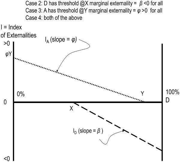
Figure 9.2. Social efficiency of hypothetical intraneighborhood externalities with thresholds: cases 2, 3, and 4
Case 3: Group A generates constant marginal positive externality φ for all neighbors beyond threshold Y (where Y is defined as maximum %D where φ persists).
Here with the “epidemic/social norm” mechanism we have the converse of case 2, with group A producing positive externalities for all if they exceed a minimum threshold of Y percent (that is, the equivalent condition is that %D falls below [100 – Y] percent). The process of social norm transmission operates here in identical fashion to that described above in case 2, except that past the threshold, socially desirable collective socialization processes ensue.
The efficiency analysis follows as above; see the IA function in figure 9.2. To maximize the sum of positive externalities, we should avoid having neighborhoods where group A households represent less than their threshold. Any A households residing in neighborhoods with less than their threshold concentration would be “wasted” from the perspective of social efficiency, since none would be producing positive externalities at this concentration. Thus, the optimal allocation would have as many A households as possible residing in neighborhoods where their concentrations exceeded the threshold. This means filling up neighborhoods completely with A households until this group is exhausted; any remaining could be allocated across the remaining neighborhoods in whatever manner. This set of assumptions in case 3 implies that an extremely segregated situation would be efficient.
Case 4: Group D generates constant marginal negative externality β for all neighbors beyond threshold X and A generates constant marginal positive externality φ for all neighbors below threshold Y (where Y is defined as maximum D where φ persists) and Y > X.
Here, from the perspective of the “epidemic/social norm” mechanism, I combine cases 2 and 3 to consider implications of the assumption that different household types produce countervailing (though not necessarily equal in magnitude) externalities that ensue at different threshold points. Figure 9.2 again applies, with ID and IA functions both operative.33
The outcome of the efficiency analysis rests on the relative magnitudes of the two externalities being generated. In this situation, inter-neighborhood variations in the household mixture in the range between the two thresholds produce a constant IT, because the net marginal externality combining both functions is a constant (following the logic of case 1). Put differently, switching group A and D households between neighborhoods that have exceeded both thresholds (and continue to do so after the hypothetical reallocation) will lead to no net change in efficiency, because the gains in the destination neighborhood will exactly offset the losses in origin neighborhood. However, whether such a mixed situation will be superior to more segregated options when one or the other threshold has not been exceeded cannot be ascertained without more information about the relative magnitudes of the two externality parameters φ and β.
Consider the following thought experiment. What would happen to efficiency if we were to reallocate some households within some of these mixed neighborhoods (that is, those with %D values between X and Y in figure 9.2) so that we instead produced more segregated neighborhoods (that is, some with %D less than threshold X, and others with %D greater than threshold Y)? If the positive externality produced by group A were much greater than the negative externality produced by group D, the set of neighborhoods with %D less than X would enjoy massive increases in positive externalities associated with now larger percentages of group A residents, with no offsetting negative externalities from group D (because their percentage would be below X). By contrast, the set of neighborhoods with %D greater than threshold X would evince some increase in negative externalities associated with their now larger percentages of D households, and no offsetting positive externalities from group A (because their percentage would be below 100 – Y). If indeed |φ|>|β|, then the gains in the former set of neighborhoods will offset the losses in the latter, and it will be more efficient for society as a whole to convert mixed neighborhoods into those that have more segregation. Following on the logic of case 3, efficiency would be maximized by allocating as many A households as possible to completely segregated neighborhoods, and then (if mathematically possible) allocating D households among any remaining neighborhoods to minimize the number that exceed threshold X.
The conclusion is the opposite if we reverse the assumptions about the relative magnitudes of the externalities and replay our thought experiment. If |φ|<|β|, then the gains in the set of previously below-threshold neighborhoods with a now larger share of group A will not offset the losses in the other set, and it will be more efficient to avoid switching mixed neighborhoods for those that have more segregation. Following the logic of case 2, efficiency here would be maximized by allocating as many D households as possible to neighborhoods with below-X concentrations and then (if mathematically possible) allocating A households among any remaining neighborhoods to maximize the number that exceed threshold Y. It is mathematically possible, of course, that the two parameters are precisely equal in absolute value, such that all allocations are equally efficient.
Case 5: Group D generates growing marginal negative externality for only D neighbors.
The externality modeled here can be considered a “selective socialization” process, wherein the assumed bad influence of one D household is felt only by other D households (not A households) in the neighborhood, perhaps because they are more vulnerable to these influences, or because the social networks of D households are homogeneous within the group and do not include any A households. Here the negative externality produced by the marginal D household increases nonlinearly with the number of D households in a neighborhood because there are more D neighbors to be affected by the externality generated by the marginal D household. Thus, the marginal negative externality can be expressed as β%D. Households in group A are assumed irrelevant as either transmitters or receivers of this externality, perhaps because they have few social networks involving group D, or because they have a great social distance from them. I show the nonlinear externality function for group D in one neighborhood, ID, in figure 9.3. In this case, allocating all group D households to neighborhoods in the smallest percentages possible, equally across all neighborhoods, would minimize the total negative externalities that they produce for themselves. That is, because the negative externality grows more than proportionately with the addition of one more group D household, for the most efficient solution, society should disperse these households in the lowest equal concentrations possible—that is, equal to their share in the overall population. If D households represented a small share of the population, this result implies that efficiency would be manifested as every neighborhood being predominantly occupied by A households. On the other hand, if D households represented half of the population (as in the simplified model), this result implies that equally mixed neighborhoods would be most efficient across the board.
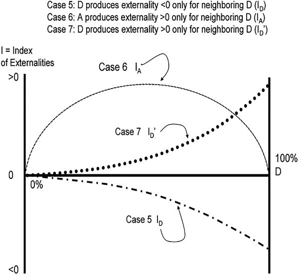
Figure 9.3. Social efficiency of hypothetical variable marginal intraneighborhood externalities: cases 5, 6, and 7
Case 6: Group A generates growing marginal positive externality for only D neighbors.
Here with the “selective socialization” mechanism, the externality produced by each A (φ) benefits each D (but not other A households) present in the neighborhood. This could represent a situation wherein each group A household provides a valuable behavioral role model for all group D households present, which is irrelevant for other group A households because they already exhibit this behavior.34 I show the corresponding IA externality function for a particular neighborhood in figure 9.3. The IA function would take on the shape of an inverted U, because eventually more A households in the neighborhood create a negative marginal impact as they reduce the number of D households present to benefit from the externality. Efficiency concerns imply that, as in case 5, the maximum positive externality overall will occur when the mix of group A and D households is identical across all neighborhoods (and equal to their respective shares in the population). The intuition is as follows. Starting with a common mix of A and D, if two neighborhoods were to switch some A and D households, the gain in positive externalities in the neighborhood losing D households would be less than the loss in positive externalities in the neighborhood gaining D households.
Case 7: Group D generates growing marginal positive externality for only D neighbors.
This variant of the “social network” mechanism describes what we might called “group affinity.” The notion implicit in this case is that as more group D households cluster in space, they can build stronger social ties within the group and build valuable cultural capital. Such might represent an “ethnic enclave” of newly arrived immigrants, for example. Here the total positive externality increases nonlinearly with the number of D in a neighborhood because there are more D neighbors to both generate and be affected by the externality. Group A households in this case are irrelevant as either transmitters or receivers of externalities. I show in figure 9.3 the group D externality function appertaining as ID.’ Efficiency considerations lead here to the opposite conclusions from those in case 5. In this case, segregation is efficient, regardless of the share of D households in the overall population. By allocating as many D households as possible to homogeneous D-occupied neighborhoods, society will achieve a higher value for IT than if society allocated D in any smaller percentages across neighborhoods. Because the marginal benefit of an added group D neighbor rises as more of group D are already present, such a household always should be added to the neighborhood with the greatest %D, up to a maximum of 100 percent.
Case 8: Group A and group D generate growing marginal positive externalities, but only for neighbors not like themselves.
This variant of the “social network” mechanism describes what we might call “social cohesion.” In this view, there may be nothing intrinsically good or bad about the behaviors and attitudes of either group, but there is a larger societal value in the social interaction between them in a neighborhood context, because it builds intergroup social capital. That is, mutual and equal positive externalities (like tolerance and empathy) are generated for all participants when they reside together; such is the essence of the “contact hypothesis.”35 I present the identical ID and IA externality functions that correspond to this case in figure 9.4. From an efficiency perspective, this is analogous to case 6, wherein both A and D produce positive externalities whose marginal benefits are proportional to those of the other group in the area. As before, the implication is that as many neighborhoods as possible should be mixed at equal percentages of group A and D households to maximize efficiency, regardless of their respective shares in the overall population.
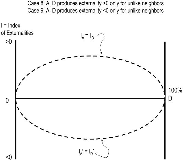
Figure 9.4. Social efficiency of hypothetical selective, variable marginal intraneighborhood externalities: cases 8 and 9
Case 9: Group A and group D generate growing marginal negative externalities, but only for neighbors not like themselves.
Here I model the “competition” neighborhood effect mechanism, which is formally equivalent to assuming that both groups have homophily preferences. Each member of both groups in this case receives disamenities from the presence of members of the other group in the neighborhood. Their common ID′ and IA′ externality functions are presented in figure 9.4. This is analyzed as the converse of case 8, wherein both A and D produce negative instead of positive externalities whose marginal benefits are proportional to those of the other group in the area. From the social efficiency perspective, one draws the conclusion that as few neighborhoods as possible should be mixed; rather group A and D households should be completely segregated, regardless of their respective shares in the overall population.
Case 10: Group D generates constant, lump-sum negative externality β for all neighbors (A and D) if D exceeds threshold Z.
This can be seen as the “neighborhood stigmatizing” mechanism. If the external marketplace holds stereotypical views about group D, it may develop negative responses toward anyone from a neighborhood where group D constitutes more than Z percent of the households, and may restrict flows of other resources to that place. Though in some sense it is not the fault of group D households that others stereotype them in this fashion, it is appropriate to model this as if they indeed were the source of this externality, even though it ultimately emanates from outside the neighborhood. I model this as a constant externality of lump-sum amount β that is imposed discontinuously once %D exceeds Z (see ID in figure 9.5).36 It is clearly more efficient in case 10 to avoid concentrations of group D households that exceed the stigmatizing threshold Z. If group D represents a small share of all households or Z is large, this well may be mathematically feasible. If not, it is preferable to allocate group D households in such a way that as many neighborhoods as possible do not exceed Z; all allocations of the remaining D will be equally efficient. Whether these efficient allocations produce mainly mixed or segregated neighborhoods will depend on the size of Z and the share of D in the overall population. If both are 50 percent, all neighborhoods should have 50 percent D and A households. If Z is small compared to the percentage of D in the population, many neighborhoods will have a large majority of A households, with only Z% of D households.

Figure 9.5. Social efficiency of hypothetical constant stigma after threshold neighborhood externalities: case 10
In summary, the foregoing makes it clear that the comparative social efficiency of alternative distributions of population groups among neighborhoods crucially depends on the nature of the externalities that they transmit to members of their own group and members of the other groups. See the second column of table 9.1 for a succinct summary of the prior ten cases’ implications for the neighborhood population composition having the greatest social efficiency. Both complete segregation and complete mixing to the extent that is arithmetically feasible emerge as potentially socially efficient outcomes, depending on the nature of the intra-neighborhood externalities (as well as the shares of groups in the overall population) being assumed. It thus becomes a critical empirical matter to ascertain which pattern of intergroup externalities appears dominant in the contemporary American context.
Note: Inequality signs indicate whether assumed intraneighborhood externality from advantaged household group A or disadvantaged household group D is positive or negative.
Inefficiencies in Households’ Mobility Behaviors: Evidence
In chapters 6, 7 and 8, I already presented the evidence relevant for assessing which of the prior hypothetical cases most closely matches the reality of most US neighborhoods, so I summarize it only briefly here. Unlike the previous theoretical discussion wherein “advantaged” and “disadvantaged” were generic terms, here it is important to distinguish the evidence related to the economic composition and the racial composition of the neighborhood.
Externalities among different economic groups. My review in chapter 8 of social interactive neighborhood effect mechanisms concluded that there was strong evidence of negative behavioral externalities created among members of economically disadvantaged groups, which manifested themselves through peer effects and collective socialization. Crucially, as I demonstrated in chapter 6, these effects typically take the form of social contagion after the concentration of the poor exceeds a critical threshold (i.e., 15 to 20 percent poverty rates).37 It is reasonable to assume that many of the behaviors generated past this threshold (such as engaging in violent or illegal activities) have negative external impacts on both economically disadvantaged and advantaged neighbors.
Additional evidence shows that poor individuals will also gain absolutely by residence near more economically advantaged neighbors. Role modeling and social control provided by economically advantaged neighbors (manifested by greater public safety), in conjunction with superior public services and institutional resources, seem more likely mechanisms of positive intra-neighborhood externalities emanating from the advantaged group.38 As I showed in chapter 8, several random assignment and natural experiments revealed that these positive externalities can be particularly powerful for younger children from poor families living among economically advantaged households.39 Evidence I reviewed in chapter 6 indicated that there likely was a threshold concentration of advantaged households in a neighborhood required to generate this positive externality, though the specific threshold parameter was uncertain.
In total, the foregoing evidence strongly suggests that (1) economically disadvantaged households create negative externalities for all neighbors once they exceed a threshold concentration, and (2) economically advantaged households create positive externalities for all neighbors once they exceed a threshold concentration. As such, this evidence points clearly toward a context as portrayed in case 4 (figure 9.2) above, though the dual marginal externalities produced past the thresholds may not be proportional as shown. Unfortunately, it is difficult from available evidence to draw any conclusions about which of the marginal magnitudes of externalities is larger. In my view, the spectrum of problems associated with concentrated disadvantage are some of the most costly we face in American society. The logical implication of this view is unambiguous. The current pattern of many American neighborhoods exceeding a poverty concentration threshold of 15 to 20 percent is socially inefficient; it yields a higher rate of unproductive and problematic behaviors for society as a whole than would be generated by alternative distributions of economic groups across neighborhoods that manifested a radically deconcentrated pattern of poverty.
How large of a social inefficiency is this? With my colleagues Jackie Cutsinger and Ron Malega, I provided a plausible lower-bound estimate using parameters from the econometric model we estimated for the causal relationship between neighborhood decadal changes in poverty rates and subsequent changes in property values and rents.40 We simulated how property values and rents would have changed in the aggregate for neighborhoods in the one hundred largest metropolitan areas, had populations hypothetically been redistributed such that two conditions were met. First, all census tracts in 1990 exceeding 20 percent poverty had their rate reduced to 20 percent by the year 2000. Second, only the lowest-poverty tracts were allocated additional poor populations, with each increasing their poverty rate by five percentage points maximum. We found in this thought experiment that owner-occupied property values would have been a staggering $421 billion (13 percent, measured in base-year 1990 dollars) greater, and monthly rents would have been $400 million (4 percent) greater in aggregate, ceteris paribus.
Externalities among different racial groups. As I discussed in chapter 7, public opinion polls and statistical studies of willingness to pay for housing consistently reveal that most black and Hispanic households prefer neighborhoods with roughly equal racial proportions. Framed in terms of externalities, this evidence suggests that black and Hispanic households residing in predominantly minority-occupied neighborhoods see new white neighbors as conveying positive externalities, at least up to the point where the neighborhood manifests as substantial diversity of races. This perception of more racially integrated environments providing positive externalities for minorities also receives support from two econometric studies demonstrating plausibly causal relationships between greater residential exposure of blacks to whites (that is, less segregation) and reduced high school dropout rates for black youths.41 This evidence is most consistent with the selective socialization mechanism, shown stylistically above in case 6 (figure 9.3).
By contrast, the same evidence from chapter 7 indicates that most whites generally prefer predominantly white-occupied neighborhoods. Opinion polls revealing whites’ negative stereotypes of individual minorities imply that they perceive more than a modest share of black or Hispanic neighbors as imposing negative externalities on them. This interpretation is also consistent with whites’ pessimistic expectations associated with predominantly black-occupied neighborhoods (as I discussed in chapter 5) and their willingness to pay more for neighborhoods that are predominantly white-occupied (as I discussed in chapter 7). Finally, the aforementioned literature on racial “tipping” strongly suggests that the magnitude of the negative externalities imposed by blacks increases on the margin as the tipping point approaches. These strands of evidence all point to a model wherein D households selectively impose increasingly negative externalities on only A households after a threshold %D has been surpassed. This is the analog of case 5 above, with the addition of a threshold.
However, additional evidence suggests that another negative externality process be included as well. Recent work by Anna Santiago and me has indicated that a variety of negative outcomes for low-income black and Hispanic youths associated with being raised in preponderantly minority-occupied neighborhoods do not mainly transpire from the racial composition per se, but rather from the correlated shortcomings in public safety, city services, and institutional investments that flow into such places.42 I think it reasonable, therefore, to posit that a threshold of disadvantaged (minority) residents is associated with this mechanism of stigmatization and altering resource flows from external forces that harm A and D households alike, so that another appropriate stylized model is case 10.
Combining the arguments of the prior two paragraphs yields a synthesized externality function for D (minority) households as portrayed as ID in figure 9.6. After surpassing threshold X, the function assumes an increasingly negative slope for reasons explained above. After %D exceeds a second threshold of stigmatization Z, however, a lump-sum of negative externality is added to this underlying function. In the range of %D > Z there is little reason from theory or evidence to believe that further increases in D concentration yield increasingly negative externalities; I therefore portray this segment as a horizontal line, for simplicity.
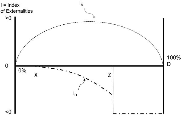
Figure 9.6. Social efficiency with combination of externalities representing current situation
In sum, the evidence points to a model of intra-neighborhood racial externalities as portrayed in figure 9.6. Two conclusions follow. The first conclusion one can draw from figure 9.6 is that a neighborhood with %D < X offers a more efficient (higher net positive externalities) alternative than one with %D > Z. In other words, neighborhoods where D households remain in the minority (assuming X < 50%) are more socially efficient than those where D constitute the overwhelming majority of residents (%D > Z). The second conclusion is that the most efficient allocation of households would be with all neighborhoods having the identical composition (equal the shares of A and D in the overall population), with one possible exception. This remarkable conclusion about the social efficiency of maximum feasible racial mixing holds quite generally within a wide range of the relative magnitudes of the offsetting positive and negative externalities, the values of the thresholds, and the relative population sizes of the two groups. Three alternatives suffice to demonstrate.
First, consider a situation where D is such a small percentage of the metropolitan area’s households that it would be mathematically feasible for all neighborhoods to house them at equal concentrations less than X percent. In this situation, we would conclude, analogously to case 6 above, that all neighborhoods with identical racial compositions would be most efficient. Starting at this distribution, consider the thought experiment of reallocating some D households such that their percentage increased in one neighborhood while decreasing in another. Given the convex curvature of the IA function, this reallocation would clearly reduce the total positive externalities since the gain in the neighborhood increasing in %D would be smaller than the loss in the one decreasing %D. This gain would be even less (perhaps even negative) were this reallocation to increase %D in the former neighborhood past X.
Second, consider a situation where D is a sufficiently large percentage of the metropolitan area’s households such that it would be mathematically feasible for all neighborhoods to house A and D at an identical concentration with %D between X and Z. This situation superficially seems more complicated with the ID function now operative, but the conclusion is the same: divergence from an identical mix across all neighborhoods reduces overall efficiency. This can be deduced from a similar thought experiment performed as above for both IA and ID functions separately, consistent with the logic in cases 5 and 6 above.
Third, consider a situation where D is such a large percentage of the metropolitan area’s households that it only would be mathematically feasible that all neighborhoods could house A and D at an identical concentration with %D > Z. Here, a thought-experimental comparison of alternative allocations among neighborhoods, all of which maintain that %D > Z, would again reveal that an identical mix across all neighborhoods maximizes overall efficiency. However, with the discontinuity in the ID function at Z, one must also compare hypothetical allocations involving some neighborhoods reducing their %D below Z. It is possible that efficiency may be enhanced by replacing two neighborhoods with identical compositions of A and D with one with %D < X and the other with a %D greater than originally, so long as the negative stigmatization externality occurring at Z (the gain the neighborhood lowering its %D) is large relative to the marginal loss in positive externality (the loss of the neighborhood raising its %D). Under such conditions, social efficiency would be maximized by having as many D households as possible allocated to one set of neighborhoods with an identical composition of D and A households (with %D slightly less than Z), and the remaining D households allocated to another set of neighborhoods that also have an identical (though different) composition of D (%D > Z) and A households.
In summary, an empirically grounded analysis based on intraneighborhood racial externalities suggests that the most socially efficient allocation of households would involve a situation in which virtually all neighborhoods in a metropolitan area would have a common racial composition, roughly matching that of the racial groups in the area as a whole. By implication, the predominant pattern of racial segregation we observe across our metropolitan areas must be socially inefficient. Unfortunately, social scientists have not agreed on how this inefficiency should manifest itself and how it should be uncovered, and thus there is far from any empirical consensus on the degree to which segregation imposes penalties on our society. Consider three realms of evidence.
First, two studies taking similar empirical approaches have come to different conclusions about whether whites gain in absolute terms (instead of just relative to minorities) from racial segregation. Ingrid Ellen, Justin Steil, and Jorge De la Roca find that individual white households living in more racially segregated metropolitan areas have higher wages, complete college at higher rates, and attain higher-status occupations than whites in desegregated areas.43 By contrast, Gregory Acs, Rolf Pendall, Mark Treskon, and Amy Khare find that neither black-white nor Hispanic-white segregation is significantly associated with median household incomes or per capita incomes of white households.44 Moreover, greater levels of black-white segregation are associated with lower bachelor’s degree attainment rates among whites and higher metro-wide homicide rates, which presumably impose costs on all groups. They also find no significant associations between whites’ median incomes, per capita incomes, or college graduation rates and economic segregation for the metropolitan area.45 They do find, however, substantial harms to minorities from segregation, as I will amplify below. Their findings thus suggest that segregation is inefficient, since some members of society lose while no one gains.
Second, several studies find that racially diverse neighborhoods score higher on some measures of unfavorable social conditions, which would argue against the inefficiency of segregation. John Hipp, for example, discovers that neighborhoods with similar housing and socioeconomic profiles have higher crime rates if they have greater racial diversity, a result he attributes to heightened senses of relative deprivation.46 Robert Putnam has observed that there are lower levels of social capital in racially diverse neighborhoods.47 Unfortunately, these studies’ conclusions about causation are not definitive, since they only observe patterns across neighborhoods, which cannot rule out the bias from selective mobility that I discussed in the previous chapter.
The third realm of evidence relevant to the social inefficiency of racial segregation is the question of whether whites’ perceptions of negative externalities from their exposure to different racial groups should unquestioningly be accepted as either socially acceptable or immutable.48 There is considerable evidence that both advantaged and disadvantaged populations may benefit from sharing the same neighborhood if the contact results in a reduction of intergroup prejudices.49 Many US studies have observed that interethnic group tolerance and subsequent social contacts expand with greater intra-neighborhood exposure, especially when they occur earlier in life.50 The “contact hypothesis,” as it is termed, implies that white’s perceptions about the putative negative externalities flowing from substantial racial diversity in neighborhoods are malleable. If indeed whites’ prejudices might wane over time from experience with more diverse neighborhoods, this would tip the balance of evidence farther toward the conclusion that racial segregation is a socially inefficient outcome.
Social Inefficiencies: Dynamic Perspective
In the last section, I examined how a static snapshot of our neighborhoods reveals socially inefficient patterns of too little property investments and too much segregation by income and by race, due to strategic gaming and externalities that led to market failures. Here I switch the focus of the inefficiency analysis to consider the dynamic process by which neighborhoods transition from one set of demographic, economic, and physical characteristics to another. Again, I will conclude that the autonomous, market-guided dynamics are inefficient from a societal perspective, this time because of self-fulfilling prophecies. A self-fulfilling prophecy in a neighborhood context is a process that starts with an individual making a decision related to residential mobility or property investment on the basis of fearful expectations. Unfortunately, if many other decision makers in the neighborhood do the same, this aggregation of actions ushers in the feared event. This is a classic example of collective irrationality: what is sensible action from the perspective of an autonomous individual proves irrational when the collective engages in the same action. Researchers have documented well these self-fulfilling prophecies in the realms of residential mobility and property reinvestment behaviors.
Racial composition-related expectations drive many of these self-fulfilling prophecies. Recall that I reviewed in chapter 5 the strong evidence indicating that whites, and often blacks, view a substantial share or large increase in the black population of a neighborhood as a harbinger of declining quality of life and property values, as summarized in the The Proposition of Racially Encoded Signals. When a large number of current residents and owners use this indicator as a basis for underinvesting in their properties and/or leaving the neighborhood, they will encourage the very racial and perhaps class succession of their neighborhoods that they pessimistically expected. Robert Sampson and Stephen Raudenbush provided a dramatic example of this dynamic.51 They observed that white residents, especially those who were better off financially, perceived more disorder in a neighborhood with larger shares of black residents, even controlling for a myriad of objective indicators of disorder. As a result, they were more likely to disinvest and move away from the neighborhood, thus ushering in more disorder. Richard Taub, Garth Taylor, and Jan Dunham documented an analogous process.52 They observed that whites’ perceptions of growing in-migration of black residents fueled concomitant expectations of eroded public safety and competitiveness of the neighborhood, which led them to cut back their upkeep activities.
Expectations regarding racial change are not required to generate inefficient self-fulfilling prophecies in neighborhoods, however. Owners who hold pessimistic expectations about the future quality of life in their neighborhood will reduce their property upkeep investments, hastening the decline they feared.53 In sum, the dynamics of neighborhood change often embody collectively irrational behaviors that produce outcomes that none of the individual decision-makers would have desired.
Social Inequities: Static Perspective
The inefficiently low levels of investment in residential properties and high levels of neighborhood segregation by race and income do not impose their costs evenly across all groups in America. On the contrary, these costs are disproportionately borne by those who have traditionally been least advantaged in our society: lower-income and minority households.54
Investigating the adverse consequences of residential segregation for ethnic minority people has a long and distinguished social scientific history.55 Over the last several decades, scholars have developed sophisticated statistical models that permit valid causal inferences to be drawn about the degree to which racial segregation produces a variety of interracial disparities in outcomes.56 These studies identified substantial and roughly equal socioeconomic and health costs that segregation imposes on blacks and Hispanics. Justin Steil, Jorge de la Roca, and Ingrid Ellen provide recent estimates of the approximate magnitudes of these harms for individual young adult minorities of the ages twenty-five to thirty.57 For black individuals, a one-standard-deviation increase in the black-white dissimilarity index of metropolitan area segregation is associated with a decline in the probability of completing high school of 1.4 percentage points relative to whites (that is, 20 percent of the difference in means between these groups). A one-standard-deviation increase in the Hispanic-white dissimilarity index is associated with an even larger decline in the probability of finishing high school of 3 percentage points for Hispanic individuals relative to white individuals (that is, 33 percent of the difference between group means). Analogously, such an increase in segregation is associated with a decline in the probability of completing college by 4.8 percentage points for blacks and 4.6 percentage points for Hispanics (representing 21 percent and 19 percent of the respective mean gaps with whites). Both blacks and Hispanics exhibit equally strong relationships between racial segregation and interracial gaps in single motherhood, in being simultaneously out of school and out of work, and in earnings.58
By contrast, there is much less causal evidence about the degree to which intermetropolitan variations in economic segregation are responsible for individual differences in socioeconomic outcomes, and how these relationships may vary by race. All the cross-sectional work here is descriptive in nature.59 Raj Chetty, Nathaniel Hendren, Patrick Kline, and Emmanuel Saez found that children growing up in metropolitan areas with higher levels of economic segregation are less likely to advance from their parents’ economic position, controlling for many other characteristics of their metropolitan area.60 Bryan Graham and Patrick Sharkey come to a similar conclusion using different data sets and measures.61 Gregory Acs, Rolf Pendall, Mark Treskon, and Amy Khare observed that blacks in metropolitan areas with lower amounts of economic segregation have significantly higher per capita incomes, median household incomes, and rates of attaining bachelor’s degrees, controlling for other characteristics of their metropolitan areas.62 Statistical studies of individual outcomes and neighborhood-level exposures to different socioeconomic groups (the “neighborhood effects” literature I summarized in chapter 8) have given us most of the substantial plausible causal evidence regarding the inequities produced by economic segregation.
Due to the synergistic operation of racial and economic segregation, neighborhood physical decay, economic deprivation, and minority composition exhibit distinctive spatial congruence in American metropolitan areas. Blacks and Hispanics are exposed, on average, to much higher incidences of neighborhood physical and socioeconomic disadvantage than whites, even when they have similar incomes.63 Several studies employing the latest census data have confirmed this conclusion in complementary ways. John Logan showed that across all metropolitan neighborhoods, the average black person is exposed to a 77 percent higher neighborhood poverty rate, than the average white person, and the average Hispanic person is exposed to a 62 percent higher poverty rate.64 The interracial gaps in neighborhood poverty exposure are even greater for poor minorities: 102 percent and 85 percent higher for blacks and Hispanics, respectively.65 Paul Jargowsky documented that 25 percent of poor blacks and 17 percent of poor Hispanics live in neighborhoods with extreme poverty rates of 40 percent or more, compared to only 7 percent of poor whites.66 These dramatic neighborhood inequalities extend across the income distribution. Patrick Sharkey found that blacks with household income of $100,000 or more live in and are nearby neighborhoods with higher levels of disadvantage than white families with income of $30,000 or less.67 Sean Reardon, Lindsay Fox, and Joseph Townsend showed that neighborhood economic conditions are the same for the average white household earning $11,800, the average Hispanic household earning $45,000, and the average black household earning $60,000.68
From the foregoing, it is abundantly clear that segregation-induced differences in exposure to neighborhood disadvantage lead ultimately to unequal socioeconomic outcomes for individuals based on their race and class.69 Yet, what is it exactly about these inequitable differentials that creates these effects? Below I briefly document five categories of unfair burdens that these disadvantaged households bear because of the segregated pattern of physical, demographic, and economic characteristics of American neighborhoods.70
Subcultural Adaptations
The spatial isolation of lower-income and racial minority groups can encourage and permit the development of distinct subcultural attitudes, behaviors, and speech patterns that may impede success in the mainstream world of work, either because they are counterproductive in some objective sense or because they are perceived to be so by prospective (typically higher-income, white) employers. Segregation makes it harder for low-income and minority children to acquire the “soft skills” valued in the labor market.71 These valuable skills, especially styles of communication and interpersonal relationships, arise primarily from social patterns prevailing in white middle-class culture. Instead, these children may develop alterative patterns that may serve them well on the streets (like cool posing and hypersensitivity to perceived disrespect)72 but hinder them in the conventional workplace.73
Reduced Wealth Accumulation via Higher Prices
Wealth is stripped from low-income and minority communities because the nature of the local retail and financial services sector renders it more expensive to live there. These communities pay more for food, primarily due to the lack of large-volume supermarkets.74 Poor neighborhoods and predominantly black neighborhoods have roughly half the number of supermarkets as do wealthy ones and white ones.75 The withdrawal of the mainstream financial services industry from disadvantaged neighborhoods has created a vacuum that has been filled by the fringe financial sector, including payday lenders, check-cashing outlets, rent-to-own stores, and pawnshops.76 Fees paid to payday lenders and check-cashing outlets for services that are normally free in better-banked communities run into the billions of dollars annually.77 One estimate calculates that average full-time workers regularly using a check cashing service would have gained $360,000 in wealth during their working lifetimes if they had saved those fees by having a checking account.78 Higher-interest subprime mortgage lending is often foisted upon minority homebuyers even when their credit scores do not justify it.79 One recent study estimates that, as compared to equally qualified white borrowers in same-quality white neighborhoods, black borrowers in predominantly black neighborhoods in Baltimore paid 6.4 percent higher monthly mortgage costs (resulting in roughly $16,000 more over the life of a thirty-year loan) as a net result of racially disparate patterns of mortgage lending.80 Insurance coverage for homes and autos is more expensive in low-income and minority-occupied neighborhoods.81 The combined effect of these excess costs of living in low-income neighborhoods has been estimated to strip away about a quarter of a poor person’s income;82 it is probably even greater if blacks or Hispanics predominantly occupy the neighborhood.
Inferior Public Services and Institutions
Not only are lower-income and minority households separated residentially from their higher-income and white compatriots; they disproportionately reside in distinct municipalities that are more financially stressed because of their combination of economic and population decline and concentrations of poverty. This means that the juxtaposition of inferior public services and high tax rates may be the unenviable situation facing such disadvantaged households. Moreover, lower-income and minority households disproportionately endure not only the worst interjurisdictional inequities in public services and facilities, but intra-jurisdictional ones as well. Many studies have documented the vast differences in both public and private institutional resources serving different neighborhoods both across and within jurisdictions,83 and there is growing consensus that such institutions serve as important mechanisms through which neighborhood effects transpire.84 As illustration, measurable educational resources vary dramatically across space and correlate strongly with several aspects of student performance.85 Black, Hispanic and low-economic-status students generally can access only inferior school resources. The average black or Hispanic public elementary school student in 1999–2000 attended a school where more than 65 percent of students were poor, compared to only 30 percent poor in the average white child’s public school.86 Shortages of high-quality childcare facilities are acute in many low-income and minority neighborhoods, despite their proven effectiveness in building a variety of intellectual and behavioral skills in young children.87 Lower-income communities are also at a disadvantage in terms of access to medical facilities and practitioners.88 Furthermore, it is clear that many low-income minority parents believe that the perceived paucity of local institutional resources adversely affects their children,89 and often try to compensate for this shortcoming by seeking them from outside of their neighborhoods.90
Unhealthy Exposures to Pollution and Violence
The physical and social environment can affect health through multiple pathways, resulting in strong disparities in morbidity and mortality across neighborhoods differentiated by race and income.91 First, undermaintained housing can create issues of physical danger (e.g., overloaded electrical systems, defective heating sources, or broken steps and railings); epidemiological problems related to drafts, mold, vermin infestations, and lead toxins;92 and a reduced sense of personal efficacy.93 Second, neighborhoods predominantly occupied by racial minorities or by lower-income households have higher concentrations of air pollution and exposure to toxic waste sites.94 One recent study found that blacks lived in neighborhoods with concentrations of toxic air pollutants that are 1.45 times greater than whites’ and 1.7 times greater than Hispanics’, on average. Expressed another way, blacks earning $50,000 or more live in neighborhoods with more air pollution that whites earning less than $10,000 per year.95 In turn, many international epidemiological studies link air pollutants to lower life expectancy, higher infant and adult mortality risks, more hospital visits, poorer birth outcomes, and asthma.96 Proximity to hazardous waste (“brownfield”) sites is associated with higher rates of mortality from cancer and other diseases.97 There are strong links between neighborhood minority racial composition and children’s elevated blood lead levels.98 Studies show that even small amounts of lead poisoning, typically produced by residue from deteriorated lead-based paint formerly used in homes, can harm infants.99 Lead poisoning also harms the mental development, IQ, and behaviors of older children.100 Third, poor minority communities often possess few recreational opportunities and healthy food sources nearby, thus raising the risks of obesity.101 Fourth, individuals’ stress levels are substantially higher in poor areas,102 yielding permanent harm to the cognitive and behavioral development of children,103 reducing the efficacy of the body’s immune system,104 and increasing rates of cardiovascular disease and premature death for adults.105 It can also produce a variety of unhealthy stress-reduction behaviors, such as smoking.106 Fifth, exposure to crime and violence is substantially higher in areas of concentrated poverty and minority occupancy.107 Youths and adults exposed to violence as witnesses or victims suffer increased stress and decline in mental health.108 Exposure to violence is linked to poorer pregnancy outcomes and low birth weight,109 poorer educational outcomes,110 and more aggressive behavior.111 Violence interacts with other aspects of the environment to erode health synergistically. It contributes directly to higher stress levels. Fear of crime encourages caregivers to keep their children indoors, reducing thereby their options for exercise and aggravating their chances of obesity.112 Youths exposed to violence smoke more, and run a higher risk of pregnancy.113 The net effect of all of these environmental mechanisms on health inequalities is stunning. Differences in neighborhood economic background account for a third or more of the variation in midlife health status; for example, a fifty-five-year old raised in a high-poverty neighborhood has about the same health as a seventy-year old raised in a low-poverty one.114
Access to Employment
Employment opportunities for minority and low-income workers may become more restricted in light of progressive decentralization of jobs (especially those paying decent wages only with modest skill requirements) in metropolitan areas, because the ability of those workers to learn about and commute to jobs declines as their proximity to them declines. Scholars have long labelled this “the spatial mismatch hypothesis.” Suggestive ethnographies have shown that low-income youths can benefit greatly from part-time employment by gaining resources, adult supervision, and routinized schedules;115 yet their neighborhoods typically have few such jobs.116 Evaluations of the Gautreaux program in Chicago showed that low-income black youths moving to the suburbs were more likely to hold jobs and earn more money than their counterparts who stayed within the city.117 Numerous rigorous statistical studies also have investigated this issue.118 This literature generally confirms that mismatch can be an important aspect of spatial opportunity differentials in at least some metropolitan areas. Distance to generic jobs may be less important than distance to jobs held by one’s own racial group, however—thus suggesting that not merely distance but the presence of ethnic-specific networks is crucial in understanding differential access to employment.119 Even if people can secure jobs, however, the associated transportation costs associated with spatial mismatch can consume up to a third of a moderate-income person’s budget, to say nothing of many valuable hours in their day.120
In summary, the foregoing evidence indicates a clear case of static inequity. The various manifestations of racial and economic segregation are inequitable because they disproportionately impose costs on black, Hispanic, and lower-income households while disproportionately denying them associated benefits.
Social Inequities: Dynamic Perspective
From a dynamic perspective, we can examine the degree to which the flows of households and financial resources across space lead to neighborhood changes that adversely affect the well-being of lower-income and minority households in disproportionate ways. I consider two domains of these dynamic social inequities: wealth disparities from housing appreciation, and involuntary mobility through residential displacement.
Wealth Disparities from Differential Homeownership and Housing Appreciation Rates
There have been dramatic, long-standing, and expanding interracial differentials in wealth: the median wealth of a white household is twenty times that of a black household and eighteen times that of a Hispanic one.121 Moreover, asset inequality is crucial in perpetuating racial inequalities in education, occupation, and income for succeeding generations.122
Housing constitutes a primary source of this wealth differential, since it is the dominant form in which the vast majority of Americans hold their wealth.123 We can decompose differentials in housing wealth into two components: intertemporal differences in rates of homeownership, and in appreciation of homes. For most of the twentieth century, minorities’ chances for owning homes were extremely limited because blatant discrimination by lenders denied them traditional sources of mortgage finance. This was often abetted by explicit federal regulations that denied mortgage insurance on the basis of even tiny numbers of minority households in neighborhoods.124 In the twenty-first century, the outright denial of mortgage credit on the basis of race has become rarer, but other discriminatory mortgage practices have arisen that make it less likely that minorities can continue to own the homes they have purchased. These practices include predatory lending: home equity loans foisted upon existing homeowners designed to extract high fees and interest rates and ultimately default, which have been concentrated in poor and minority neighborhoods.125 By differentially exacerbating the chances of home foreclosure, new forms of racially discriminatory mortgage lending have systematically stripped housing wealth from minority households and the neighborhoods in which they live. As illustration, Jacob Rugh, Len Albright, and Douglas Massey estimated that, in comparison to equally qualified white borrowers owning homes in same-quality white neighborhoods, black borrowers owning in predominantly black neighborhoods in Baltimore experienced a 7.9-percentage-point higher chance of foreclosure over the first decade of the twenty-first century. They also suffered a loss of two million dollars in accrued home equity due to home repossession. The authors traced these severe consequences to the racially disparate patterns of mortgage lending by one major lender alone.126 Their estimates do not include the substantial externality costs imposed by foreclosures on the value of nearby properties, as I documented earlier in this chapter.127
The second component of housing wealth differentials is the different rates at which peoples’ homes appreciate over time, based on their distinctive neighborhood contexts. This component is more central to the issue of neighborhood dynamic inequity. Put differently, to what degree do the flows of households and financial resources across space that lead to neighborhood change affect the ability of different racial groups to gain wealth through the appreciation of property they own? The answer is that it affects it to a substantial degree, according to the initial level and subsequent change in the economic and racial composition of the neighborhood.
A substantial and consistent body of evidence makes it clear that properties in neighborhoods with either a higher share of poor households or an increase in such a share experience less appreciation.128 Chenoa Flippen has documented clear patterns of differential home appreciation for owners across American metropolitan areas according to the poverty composition of the neighborhood at the time the property was purchased and the way in which it then changed, controlling for various other household and neighborhood characteristics.129 Illustrative of the magnitude of these differentials, she found that dwellings appreciated 30 percent less when the initial percentage of poor residents exceeded 30 percent (compared to those in neighborhoods with poverty rates below 5 percent). They appreciated 15 percent less if the neighborhood’s poverty rate increased by more than ten percentage points since time of purchase (compared to those with no increase in poverty).
A similar empirical consensus exists for the negative impact on appreciation of higher or growing shares of black households in the neighborhood.130 Flippen finds that dwellings appreciated 10 percent less when the initial percentage of black residents exceeded 65 percent (compared to those in neighborhoods with no black residents); they appreciated 7 percent less if their neighborhood’s share of blacks increased by more than ten percentage points after time of purchase (compared to those with no increase).131
The evidence provides a murkier picture regarding the impact of Hispanic neighborhood composition on home appreciation. Higher initial shares of Hispanic households in the neighborhood are generally associated with substantially lower rates of appreciation.132 By contrast, growing shares of Hispanics appear to boost home values somewhat.133 Flippen estimates that dwellings appreciated 28 percent less when the initial percentage of Hispanic residents exceeded 10 percent (compared to those in neighborhoods with no Hispanic residents); they appreciated 13 percent more if their neighborhood’s share of Hispanics increased by more than five percentage points since time of purchase (compared to those with no increase).134
Though the evidence is strong that home appreciation is decidedly less in neighborhoods with substantial shares of poor, black, or Hispanic residents, it is less clear about why this is the case. Several factors undoubtedly contribute. As I documented in chapter 7 and summarized in the Principle of Racially Encoded Signals, most white households are reluctant to shop for housing in neighborhoods with more than trivial shares of black or Hispanic residents, thus reducing aggregate demand for such places. As noted above, discriminatory mortgage terms proffered by lenders may erode effective demands by potential minority homebuyers. Risky loans and concomitant foreclosures differentially are concentrated in minority neighborhoods, thereby generating negative property value externalities. Perceptions of impending racial transitions may inspire “panic selling” of homes by white owners. Other owners, foreseeing such transitions, will cut back on the maintenance of their properties. Such responses produce self-fulfilling prophecies of property value depreciation, as I have explained above. In concert, these forces limiting appreciation in substantially minority-occupied neighborhoods render them more vulnerable to downward succession by lower-income groups, as researchers have documented.135 Such succession will eventually raise the neighborhood’s poverty rates and, as the prior evidence indicates, will thereby further magnify the deflating impact on property values in a synergistic fashion. The net effect of these factors is to constrain the flows of households (especially white, nonpoor ones), of investments by property owners, and of investments by financial institutions in a collective fashion that limits the ability of dwelling owners in minority and low-income neighborhoods to enjoy an amount of property value appreciation equivalent to that enjoyed by owners in other neighborhoods.
This dynamic social inequity clearly is borne disproportionately by black and Hispanic homeowners in racially diverse and predominantly minority neighborhoods. The evidence is unambiguous that black and Hispanic homeowners have indeed experienced, on average, significantly less appreciation than white homeowners, and have suffered greater losses in value when the housing market has declined.136 Flippen has simulated, for example, that if the average black homeowner were to live in a neighborhood with the same characteristics as the average white homeowner, the home would be worth 39 percent more; the corresponding figure for the average Hispanic homeowner is 76 percent more!137
It is less certain, however, whether this burden of differential appreciation is disproportionately borne by lower-income property owners. First, there is no definitive information about the income distribution of owner occupiers and absentee owners of residential properties, and how such distributions vary by the racial and economic composition of neighborhoods where their properties are located. Second, the evidence on whether lower-valued or higher-valued properties generally appreciate at a higher rate is conflicting, so even rough inferences are problematic.138
Involuntary Mobility through Residential Displacement
The second dynamic social inequity issue is the degree to which the process of upward succession (or “gentrification”) of neighborhoods (introduced in chapter 4) imposes severe burdens on the original lower-income (often minority) residents. That is, does the in-migration of higher-income (typically white) households lead to the wholesale and involuntary outmigration (or displacement) of the original residents, and the imposition of other monetary and nonmonetary costs on those who remain?
There is a substantial body of scholarship that addresses this question, which employs investigative strategies ranging from ethnographies conducted in particular case study neighborhoods to multivariate statistical models estimated on nationwide metropolitan datasets.139 There is no doubt that gentrification is becoming a more prominent feature of American neighborhoods during the twenty-first century.140 What is more in doubt is the degree to which this dynamic harms the original residents of these revitalizing neighborhoods.
Rents and property values in revitalizing neighborhoods rise due to active dwelling upgrading by owners to serve a higher-income clientele, and to passive upgrading as rents capitalize the higher-valued neighborhood physical conditions and socioeconomic profile for all dwellings, regardless of whether they are structurally improved themselves. In principle, this process could easily “force out” the original tenants who can no longer afford these higher rents.141 Two empirical challenges bedevil this deceptively simple proposition. First, how much rents increase in gentrifying areas is often difficult to ascertain, because of the lack of detailed, up-to-date, small-area data on rents. Second is the challenge of specifying the counterfactual: How many would have moved even in the absence of these rent increases? Many studies have investigated this question using different data sets and methods of statistical analysis, yet they have reached a common conclusion: Residential turnover in gentrifying neighborhoods is not substantially higher than that in equivalent, lower-income neighborhoods that do not gentrify.142 That is, involuntary displacement may not be very frequent because lower-income households move frequently as a matter of course, for a variety of reasons unrelated to rent increases. Research by Lei Ding, Jackelyn Hwang, and Eileen Divringi, analyzing where people live after they move from gentrifying areas, implies, however, that some involuntary displacement is occurring.143 They found that lower-income households in gentrifying neighborhoods are more likely to move to lower-income neighborhoods than are similar households moving from areas that are not gentrifying, especially when housing cost increases are greater in the original neighborhood.
Even if higher rents do not force them to move, lower-income residents of gentrifying neighborhoods will often see their rent burdens and the prices of local retail goods and services inflating.144 Though more difficult to quantify, a variety of nonmonetary costs for original residents also have been documented. These costs take the form of reductions in political power, civic engagement, and “cultural displacement”: a change in the aggregate neighborhood norms, preferences, retail sector, and service amenities.145 These social dynamics often can lead to a rise in social tensions within the neighborhood.146
In fairness, however, several sorts of benefits accrue to lower-income residents who remain in gentrifying neighborhoods. There appears to be an improvement in their economic circumstances, as revealed by several measures of income and credit scores,147 though the evidence on overall employment growth in gentrifying neighborhoods and other processes through which these improvements emerge is ambiguous.148 Gentrification is typically associated with increased feelings of safety and satisfaction, and more amenities enjoyed by lower-income residents.149 Finally, homeowners (many modest-income minorities) see more growth in their home equity.150
In sum, conclusions about dynamic inequities associated with neighborhood gentrification are not clear-cut. Some lower-income and minority residents have certainly experienced involuntary relocation. As a result, they have borne substantial out-of-pocket and other costs, such as disruption of social ties and residence in worse neighborhoods. However, it is uncertain how many such involuntary moves have been generated by gentrification. The alteration in the well-being of those who remain is even more ambiguous, due to the mixed evidence about the various gains and losses that have been borne.
Inefficiencies, Inequities, and Cumulative Causation
We should now step back and gain a holistic perspective on the issues I have discussed. I visually represent this view in figure 9.7. In chapter 7, I demonstrated how a mutually reinforcing nexus of causal processes encourages the segregation of our neighborhoods and schools by race and economic class, as encapsulated in figure 7.2. I diagrammatically represent these synergistic forces of race and class prejudices, discrimination, local political jurisdiction fragmentation and segregationist policies, and intergroup differences in housing purchasing power on the left-hand side of figure 9.6. In this chapter I have argued that systematic underinvestment in our housing stock and the population flows that yield segregation of neighborhoods are not efficient from the standpoint of society as a whole, and are especially burdensome to lower-income black and Hispanic households. In particular, I have documented how such disadvantaged households bear an unfair burden in the form of subcultural adaptations, reduced wealth accumulation, inferior public and private services and institutional resources, intensified exposures to unhealthy and violent environments, and atrophied access to employment appropriate to their skill levels. I summarily represent these relationships by the dotted arrows in the center of figure 9.7. In chapter 8 I explained how and why the characteristics of neighborhoods influence individuals and presented evidence about the strength of these neighborhood effects. Here I advance these arguments to reinforce my earlier point, made in chapter 8, that these multidimensionally inferior neighborhood contexts faced by disadvantaged households serve to perpetuate their disadvantaged socioeconomic status, both directly and indirectly, by influencing their life choices. I represent this result by the dashed arrows on the right of figure 9.7.
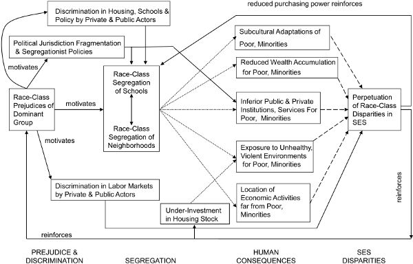
Figure 9.7. Cumulative causation among race, class, segregation, and underinvestment
These interrelationships between inefficient and inequitable patterns in our neighborhoods are even more insidious because they are mutually reinforcing.151 I represent this diagrammatically by introducing feedback loops into figure 9.7, labeled “reinforces.” First, race and class disparities in socioeconomic status contribute to the segregation of neighborhoods by making it less financially feasible for those of more modest purchasing power to afford housing in places where those with higher incomes bid up prices. As I explained in chapter 7, greater spatial clustering of dwellings representing a narrow range of market valuations (often abetted by exclusionary zoning practices) will translate into greater economic segregation when the economic gaps among households are wider. Moreover, such intensified clustering of similarly valued dwellings will generate greater segregation by race as well, because of interracial differences in income and wealth distributions. Second, race and class disparities lead to underinvestment in residential properties. The existence of a large number of poor households, of course, creates a demand for low-quality housing, as I illustrated via the Housing Submarket Model in chapters 3 and 4. Moreover, expectations strongly influenced by racial change in the neighborhood guide dwelling owners’ investments, as embodied in the Principle of Racially Encoded Signals presented in chapter 5. Third, race and class disparities reinforce the prejudices held by the dominant group—typically nonpoor whites of European ancestry—as shown by the arrow running from right to left at the bottom of figure 9.7. Many whites perceive blacks and Hispanics as less willing to work, more prone to get involved with gangs and drugs, less intelligent and educated, and less able to speak English well.152 To the extent that some empirical reality supports these stereotypical beliefs, it is precisely the reality epitomized by the human consequences that emanate from residing in their spatial niche of the metropolitan spatial opportunity structure.
Prejudices, of course, motivate a variety of behaviors by whites, as shown by the arrows labeled “motivates” in figure 9.7. Prejudice directly reinforces segregation in neighborhoods and schools through white “flight” and “avoidance.” As I have documented in chapter 6, many whites leave neighborhoods and schools when they exceed a threshold percentage of minorities or poor, and avoid such contexts when searching for alternative residential locations. Prejudice indirectly reinforces segregation in three ways. First, it incentivizes illegal behaviors by private housing market agents and landlords (like exclusion and steering), because agents will see it as more profitable to cater to the prejudices of their white clientele by preserving their homogeneous neighborhoods via discrimination.153 Similar motivations have led public officials to adopt discriminatory policies related to public housing urban redevelopment, schools, and other public sector domains.154 Second, it encourages the fragmentation of local governmental jurisdictions so that the forces of local political action and public policies (like exclusionary zoning) can mobilize more effectively to preserve the privileged status of their neighborhoods. In turn, this local political fragmentation is a prerequisite for the interjurisdictional fiscal disparities that, as I noted above, drive much of the inferior public services and schools that disadvantaged neighborhoods must suffer. Third, it leads to discrimination in labor markets related to the employment, retention, compensation, and promotion of minorities. Clearly, this feeds back to intensify further the initial interracial disparities in socioeconomic status.
To summarize the picture of cumulative causation in figure 9.7 more simply: We have created a metropolitan opportunity structure consisting of warped space. Its primary linchpin is race-class segregation of neighborhoods and schools, abetted by underinvestment in the housing stock. This opportunity structure directly erodes the mental and physical health of disadvantaged households, reduces their ability to access jobs and accumulate wealth, and degrades the quality of services and institutions with which they come into contact—all because of the neighborhoods in which they must reside. It indirectly induces many lower-income minority households residing in these disadvantaged neighborhoods to undertake behaviors that are rational within their constrained set of options, but which ultimately serve to perpetuate their socioeconomic inferiority. In turn, these behaviors legitimize prejudices held by the dominant group against lower-income and minority households, motivating and justifying in the view of the dominant group legal and illegal acts and structures in housing markets and local political jurisdictions that reinforce segregation and underinvestment in disadvantaged neighborhoods.
The Propositions of Inefficiency, Inequity, and Unequal Opportunity
I succinctly summarize the foregoing analysis in three propositions:
Inefficiency: Private, market-oriented decision makers governing resource flows among neighborhoods usually arrive at an inefficient allocation due to externalities, strategic gaming, and self-fulfilling prophecies, systematically producing too little investment in housing and too much segregation by race and economic standing.
Inequity: Lower-socioeconomic-status black and Hispanic households and property owners typically bear a disproportionate share of the financial and social costs associated with segregation, underinvestment, and neighborhood transition processes while reaping comparatively little of their social benefits.
Unequal opportunity: Because neighborhood context powerfully affects children, youth, and adults—while neighborhood contexts are very unequal across economic and racial groups—space becomes a way of perpetuating unequal opportunities for social advancement.
Conclusion
Our market-dominated system for determining the flows of human and financial resources across neighborhoods has produced a systematic bias toward too little investment in housing and too much segregation by race and economic standing, both of which are socially inefficient and inequitable. Inefficiencies arise primarily due to the presence of externalities of several sorts, strategic gaming, and self-fulfilling prophecies. Inequities arise because disadvantaged residents disproportionately confront neighborhoods that are inferior in many domains. The forces that maintain this inefficient and inequitable neighborhood system are intertwined in a mutually reinforcing system of cumulative causation that serves to perpetuate race and class disparities in America.
If ever there were a classic illustration of pernicious market failure, it is here. Thus, there is a prima facie case for collective intervention in markets through public policy, and planning for rectifying these inefficient and inequitable outcomes. I consider principles and practices for doing so next.