1 How to Get Causes from Probabilities
Abstract: In the context of linear causal systems, 'How to Get Causes from Probabilities' shows that given correct background information about other causal facts, certain probabilistic relations (like correlations and partial correlations) are both necessary and sufficient for the truth of new causal facts. This is done by showing how simple structural models from econometrics can be read causally if the conditions for identification of the model are met, and a generalized version of Reichenbach's principle of the common cause is assumed.
Nancy Cartwright
1.1. Introduction
How do we find out about causes when we cannot do experiments and we have no theory? Usually we collect statistics. But how do statistics bear on causality? The purest empiricism, following David Hume, supposes that general causal truths can be reduced to probabilistic regularities. Patrick Suppes provides a modern detailed attempt to provide such a reduction in his probabilistic theory of causality.
1Others working on probabilistic causality reject empiricist programmes such as Suppes' altogether. Wesley Salmon is a good example. For a long time Salmon tried to characterize causation using the concept of statistical relevance. But he eventually concluded: 'Causal relations are not appropriately analysable in terms of statistical relevance relations.'
2Salmon now proposes to use concepts that have to do with causal processes, like the concepts of propagation and interaction. What then of statistics? When causes no longer reduce to probabilities, why do probabilities matter?
This chapter aims to answer that question in one particular domain—roughly the domain picked out by linear causal modelling theories and path analysis. It is widely agreed by proponents of causal modelling techniques that causal relations cannot be analysed in terms of probabilistic regularities. Nevertheless, statistical correlations seem to be some kind of indicator of causation. How good an indicator can they be? The central thesis of this chapter is that in the context of causal modelling theory, probabilities can be an entirely reliable instrument for finding out about causal laws. Like all instruments, their reliability depends on a number of background assumptions; in this particular case, where causal
end p.11
conclusions are to be drawn, causal premisses must be supplied. Still, the connection is very strong: given the right kind of background information about other causal facts, certain probabilistic relations are both necessary and sufficient for the truth of new causal facts.
This interpretation of causal modelling theory is controversial. Many social scientists simply assume it and set about using modelling theory to draw causal conclusions from their statistics and to teach others how to do so. Others are more explicit: Herbert Asher in
Causal Modelling claims: 'Both recursive and non-recursive analysis procedures allow one to conclude that a causal relationship exists, but the conclusion holds only under a restrictive set of conditions.'
3Another example is the book
Correlation and Causality by David Kenny. Although at the beginning Kenny puts as a condition on causality that it be 'an active, almost vitalistic, process',
4this condition plays no role in the remainder of the book, and only two pages later he argues that causal modelling, when properly carried out, can provide causal conclusions:
A third reason for causal modelling is that it can provide a scientific basis for the application of social science theory to social problems. If one knows that X causes Y, then one knows that if X is manipulated by social policy,
ceteris paribus, Y should then change. However if one only knows that X predicts Y, one has no scientific assurance that when X is changed, Y will change. A predictive relationship may often be useful in social policy, but only a causal relationship can be applied scientifically.
5By contrast, a large number of other workers argue that no such thing is possible. Consider, for example, Robert Ling's highly critical review of Kenny's book:
[According to Kenny] the path analyst is supposed to be able to extract causal information from the data that other statisticians such as myself cannot, simply because of the additional causal assumption . . . placed on the model.
6Ling maintains that Kenny's attempt to infer causes from statistics has a serious 'logical flaw'.
7He thinks that the derivation of any
end p.12
causal claim is a 'logical fallacy'
8and concludes: 'I feel obliged to register my strongest protest against the type of malpractice fostered and promoted by the title of this book.'
9 This chapter will argue that causality is not a malpractice in statistics: given the kinds of very strong assumption that go into causal models, it is possible to extract causal information from statistics. This defence does not, of course, counter the familiar and important criticisms made by many statisticians,
10that the requisite background assumptions are not met in most situations to which social scientists try to apply causal models; nor does it address questions of how to estimate the 'true' probabilistic relations from available data. In addition there will, not surprisingly, be a number of caveats to add. But the broad import of the conclusions here is that you can indeed use statistics to extract causal information if only the input of causal information has been sufficient.
1.2. Determining Causal Structure
Econometrics is surely the discipline which has paid most attention to how functional laws, probabilities, and causes fit together. For econometrics deals with quantitative functional laws, but it is grounded in a tradition that assumes a causal interpretation for them. Moreover, it is with econometrics that probabilities entered economics. So econometrics is a good starting-place for a study of the relationship between causes and regularities.
I say I begin with econometrics, but in fact I am going to describe only the most primitive structures that econometrics provides. For I want to concentrate on the underlying question 'How do causes and probabilities relate?' To do so, I propose to strip away, as far as possible, all unnecessary refinements and complications. In the end I am going to argue that, at least in principle, probabilities can be used to measure causes. The simple structural models I take from econometrics will help show how. But there is, as always, a gap between principle and practice, and the gap is unfortunately widened by the
end p.13
drastic simplifications I impose at the start. It is not easy to infer from probabilities to causes. A great deal of background information is needed; and more complicated models will require not only fuller information but also information which is more subtle and more varied in kind. So the practical difficulties in using the methods will be greater than may at first appear. Still, I want to stress, these are difficulties that concern how much knowledge we have to begin with, and that is a problem we must face when we undertake any scientific investigation. It is not a problem that is peculiar to questions of causality.
The methods of econometrics from which I will borrow are closely connected with the related tool of path analysis, which is in common use throughout the social and life sciences. I concentrate on econometric models rather than on path analysis for two reasons. The first is that I want to focus on the connection, not between raw data and causes, but between causes and laws, whether the laws be in functional or in probabilistic form. This is easier in econometrics, since economics is a discipline with a theory. Econometrics attempts to quantify the laws of economics, whereas the apparently similar equations associated with path analysis in, for example, sociology tend to serve as mere descriptive summaries of the data. Hence the need to be clear about the connection between causes and laws has been more evident in econometrics.
My second reason for discussing econometrics is related to this: the founders of econometrics worried about this very problem, and I think their ideas are of considerable help in working out an empiricist theory of causality. For they were deeply committed both to measurement and to causes. I turn to econometrics, then, not because of its predictive successes or failures, but because of its comparative philosophical sophistication and self-consciousness. The basic ideas about causal modelling in econometrics will be used in this chapter; and many of the philosophical ideas will play a role in Chapters
3 and
4.
Although econometricians had been using statistical techniques in the 1920s and 1930s, modern econometrics, fully involved with probability, originated at the very end of the 1930s and in the 1940s with the work of Jan Tinbergen, Tjalling Koopmans, and Trygve Haavelmo.
11The methods that characterize econometrics in the
end p.14
USA, at least until the 1970s, were developed in the immediate post-war years principally at the Cowles Commission for Research in Economics, where both Koopmans and Haavelmo were working. The fundamental ideas of probabilistic econometrics were seriously criticized from the start. The two most famous criticisms came from the rival National Bureau of Economic Research and from John Maynard Keynes. The NBER practised a kind of phenomenological economics, an economics without fundamental laws, so its ideas are not so relevant to understanding how laws and causes are to be connected. To study this question, one needs to concentrate on those who believe that economics is, or can be, an exact science; and among these, almost all—whether they were econometricians or their critics—took the fundamental laws of economics to be causal laws.
Consider Keynes's remarks, near the beginning of his well-known critical review of Tinbergen's work on business cycles:
At any rate, Prof. Tinbergen agrees that the main purpose of his method is to discover, in cases where the economist has correctly analysed beforehand the qualitative character of the causal relations, with what strength each of them operates . . .
12Tinbergen does not deny that his method aims to discover the strength with which causes operate. But he does think he can pursue this aim successfully much further than Keynes admits. Given certain constraints on the explanatory variables and on the mathematical forms of the relations, '
certain details of their "influence" can be given . . . In plain terms: these influences can be measured, allowing for certain margins of uncertainty.'
13Notice that Tinbergen here uses the same language that I adopt: probabilities, in his view, work like an instrument, to
measure causal influences. Later in this section I will present a simple three-variable model from Herbert Simon to illustrate how this is done.
Criticisms similar to Keynes's had already been directed against earlier statistical methods in econometrics, notably by Lionel Robbins in his well-known Essay on the Nature and Significance of Economic Science. Robbins argued, as Keynes would later, that the causes which operate in economics vary across time:
end p.15
The 'causes' which bring it about that the ultimate valuations prevailing at any moment are what they are, are heterogeneous in nature: there is no ground for supposing that the resultant effects should exhibit significant uniformity over time and space.
14Robbins does not here reject causes outright, but he criticizes Tinbergen and the other econometricians on their own ground: the economic situation at any time is fixed by the causes at work in the economy. One may even assume, for the sake of argument, that each cause contributes a determinate influence, stable across time. Nevertheless, these causes may produce no regularities in the observed behaviour of the economy, since they occur in a continually changing and unpredictable mix. A cause may be negligible for a long time, then suddenly take on a large value; or one which has been constant may begin to vary. Yet, despite Robbins's doubts that the enterprise of econometrics can succeed, his picture of its ontology is the same as that of the econometricians themselves: econometrics studies stable causes and fixed influences.
To see how the study proceeds I begin with a simple example familiar to philosophers of science: Herbert Simon's well-known paper 'Spurious Correlation: A Causal Interpretation',
15which is a distillation of the work of earlier econometricians such as Koopmans. The paper starts from the assumption that causation has a deterministic underpinning: causal connections require functional laws. The particular functional relations that Simon studies are linear. There is a considerable literature discussing how restrictive this linearity assumption is, but I will not go into that, because the chief concern here is clarity about the implications even granted that the linearity condition is satisfied. I will also assume that all variables are time-indexed, and that causal laws are of the form '
X tcauses
Y t + Δ t, where
t > 0. I thus adopt the same view as E. Malinvaud in his classic text
Statistical Methods in Econometrics. Malinvaud says that cyclical causal relations (like those in Fig.
1.1) arise only
because we have disregarded time lags . . . If we had related the variables to
end p.16
time, the diagram would have taken the form of a directed chain of the following type:
It would now be clear that
Y tis caused by
P t − 1and causes
P t + 2.
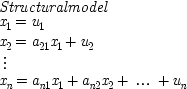
16 This assumption plus the assumption that causally related quantities are linear functions of each other generates a 'recursive model', that is, a triangular array of equations, like this:
Here each
x iis supposed to have a time index less than or equal to that for
x i + 1, and only factors with earlier indices occur on the right-hand side of any equation. For short, factors on the right-hand side in a structural equation are called the
exogenous variables in that equation, or sometimes the
independent variables; those on the left are
dependent. The
us have a separate notation from the
xs because they are supposed to represent unknown or unobservable factors that may have an effect.
end p.17
The model is called 'structural' because it is supposed to represent the true causal structures among the quantities considered. Its equations are intended to be given the most natural causal interpretation: factors on the right are causes; those on the left are effects. This convention of writing causes on the right and effects on the left is not new, nor is it confined to the social sciences; it has long been followed in physics as well. Historian of science Daniel Siegel provides a good example in his discussion of the difference between the way Maxwell wrote Ampère's law in his early work and the way it is written in a modern text. Nowadays the electric current,
J, which is treated as the source of the magnetic field, is written on the right—but Maxwell put it on the left. According to Siegel:
The meaning of this can be understood against the background of certain persistent conventions in the writing of equations, one of which has been to put the unknown quantity that is to be calculated—the answer that is to be found—on the left-hand side of the equation, while the known or given quantities, which are to give rise to the answer as a result of the operations upon them, are written on the right-hand side. (This is the case at least in the context of the European languages, written from left to right.) Considered physically, the right- and left-hand sides in most cases represent cause and effect respectively. . .
17In the context of a set of structural equations like the ones pictured here, the convention of writing effects on the left and causes on the right amounts to this: an early factor is taken to be a cause of a later, just in case the earlier factor 'genuinely' appears on the right in the equation for the later factor—that is, its coefficient is not zero. So one quantity, x i, is supposed to be a cause of another, x j(where i<j), just in case a ji≠ 0. Grant, for the moment, that for each n, U nis independent of the other causes of x n, in all combinations. If so, it will be possible to solve for the values of the parameters a jiin terms of the joint probabilities of the putative causes, and thus to determine which parameters are zero and which are not. But this means that it is possible to infer whether an earlier factor is really a cause of a later factor or not just by looking at the probabilities. This is the point of Simon's paper.
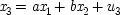
Consider, for example, the three-variable case which Simon discusses:
end p.18
and imagine that
x 2is correlated with
x 3. Does
x 2really cause
x 3, or is the correlation spurious? To claim it is spurious is not to say that the correlation itself is not genuine, but rather that the causal relation it suggests is false:
x 2does not in fact cause
x 3; the correlation between them occurs because they are both effects of the common cause
x 1. According to the convention adopted for reading equations like Simon's,
x 2will be a genuine cause of
x 3just in case
b ≠ 0. (Similarly,
x 1is a genuine cause if
a ≠ 0.) What probabilistic relations must hold for this to be the case?
My discussion will differ from Simon's. His calculations involve joint expectations, for example Exp (
x 2x 3), whereas I will solve for
b in terms of the expectations
conditional on fixed values of
x 1, like Exp (
x 2x 3/
x 1). I do so because the expression for the parameters
a and
b will then be in the form most common in the philosophical literature on probabilistic causality, as well as in the discussion of certain no-hidden-variables proofs in quantum mechanics, which will be described in the last chapter. To solve for
b, first note that
and
Using the independence of
u 3from
x 1and
x 2and scaling the error term so that its expectation is zero, this gives
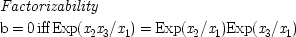
18This means that
x 2is not a cause of
x 3just in case their joint expectation factors when
x 1is held fixed. In that case the operation of
x 1as a joint cause for both
x 2and
x 3remains as the only possible account for whatever correlations exist between the two. Hence this criterion is often referred to as the 'common-cause condition'. When more than three variables are involved factorizability continues to mark the absence of a direct influence of one variable on another, only in this case not just
x 1but all the alternative possible causes of the effect-variable must be held fixed. The parameter
a can be solved for in a
end p.19
similar way. It is also easy to generalize to models with more variables. The formulae become more complicated, but as long as the assumptions of the model are satisfied it is always possible to solve for the parameters in terms of the probabilities. It looks, then, as if causes can indeed be inferred from probabilities.
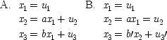
But there is a stock objection: the bulk of Simon's paper is devoted to showing that the parameters can be determined from the probabilities. But the problem occurs one stage earlier, in the interpretation of the data and the selection of variables. The argument given here assumes, roughly, that dependent variables are effects and independent variables are causes. But the facts expressed in a system of simultaneous equations do not fix which variables are dependent and which are independent. Consider for example the equations
These two sets of equations are equivalent assuming
b′ = (
b/
a) and
u 3′ =
u 3− (
b/
a)
u 2. Yet they represent different, incompatible causal arrangements. Since Simon seems to argue that causes can be inferred from correlations (when the conditions of the model are met), it is well to look at what he has to say about this problem.
Rather than looking immediately at Simon's work itself, it is instructive to consider a short, non-technical summary of it. The summary is taken from a collected set of student notes from a class on causal modelling taught by Clark Glymour.
19The notes provide an extremely clear and concise statement of one interpretation of Simon's view and the difficulties it meets. They begin by looking at sets of equivalent equations, like A and B above, which seem to yield different causal pictures. This raises a serious problem for any attempt to ground causal claims purely in functional relationships: 'If altering the equations to a mathematically equivalent set alters the causal relations expressed, then those relations involve additional structure not entirely caught by the equations alone.'
20 The equations from the Glymour notes are:
end p.20
In these equations:
These, unlike the previous equations, leave no space for omitted factors or random errors—there are no
us—hence they describe a fully deterministic system. Still, they are intended to be read in the same way: in
iv , the variables
y 1and
y 2are causally unordered; in
v ,
y 1causes
y 2; and in
vi , the two are causally independent.
The notes continue:
Simon recognizes this problem and offers a solution. He says that if an alteration is made in one of the coefficients of an equation in a linear structure and there exists a variable in that equation whose value is unaltered by the variation, then that variable is exogenous with respect to the other variables in the system. In system iv , 'wiggling' any of the coefficients in the first equation produces a change in both y 1and y 2. The same is true of the second equation. This system can therefore provide no information about which variable is exogenous. However, in the equivalent system v , if a 21, a 22, or a 20is varied, the value of y 2will be altered, but y 1will not be; therefore, y 1is the exogenous variable under Simon's criterion. This means that y 1causes y 2. System vihas only one variable in each equation; hence it cannot provide us causal information by this criterion. Simon's contention is that the equivalent system that provides causal ordering in this way is the one that identifies the actual causal relations.
To see that this additional criterion fails to resolve the difficulty, consider the following system which is also equivalent to the three above:
Using Simon's new criterion, these equations identify
y 2as the independent causal variable because varying any of the coefficients in the second equation produces a change in
y 1but not
y 2. Using this sort of rearrangement, it is possible to find equivalent systems for any system of equations in which the causal relations identified by Simon's criteria are completely rearranged.
21end p.21
So this strategy fails. I do not think that Simon's 'wiggling' criterion was ever designed to solve the equivalence problem. He offered it rather as a quasi-operational way of explaining what he meant by 'causal order'. But whether it was Simon's intent or not, there is a prima-facie plausibility to the hope that it will solve the equivalence problem, and it is important to register clearly that it cannot do so.
Glymour himself concludes from this that causal models are hypothetico-deductive.
22For him, a causal model has two parts: a set of equations and a directed graph. The directed graph is a device for laying out pictorially what is hypothesized to cause what. In recursive models it serves the same function as adopting the convention of writing the equations with causes as independent variables and their effects as dependent. This method is hypothetico-deductive because the model implies statistical consequences which can then serve as checks on its hypotheses. But no amount of statistical information will imply the hypotheses of the model. A number of other philosophers seem to agree. This is, for instance, one of the claims of Gurol Irzik and Eric Meyer in a recent review of path analysis in the journal
Philosophy of Science: 'For the project of making causal inferences from statistics, the situation seems to be hopeless: almost anything . . . goes.'
23 Glymour's willingness to accept this construal is more surprising, because he himself maintains that the hypothetico-deductive method is a poor way to choose theories. I propose instead to cast the relations between causes and statistics into Glymour's own bootstrap model: causal relations can be deduced from probabilistic ones—given the right background assumptions.
24But the background assumptions themselves will involve concepts at least as rich as the concept of causation itself. This means that the deduction does not provide a source for reductive analyses of causes in terms of probabilities.
The proposal begins with the trivial observation that the two sets of equations, A and B, cannot both satisfy the assumptions of the model. The reason lies in the error terms, which for each equation
end p.22
are supposed to be uncorrelated with the independent variables in that equation. This relationship will not usually be preserved when one set of equations is transformed into another: if the error terms are uncorrelated in one set of equations, they will not in general be uncorrelated in any other equivalent set. Hence the causal arrangement implied by a model satisfying all the proposed constraints is usually unique.
But what is the rationale for requiring the error terms to be uncorrelated? In fact, this constraint serves a number of different purposes, and that is a frequent source of confusion in trying to understand the basic ideas taken from modelling theory. It is important to distinguish three questions: (1) The Humean problem: under what conditions do the parameters in a set of linear equations determine causal connections? (2) The problem of identification (the name for this problem comes from the econometric literature): under what conditions are the parameters completely determined by probabilities? (3) The problem of estimation: lacking knowledge of the true probabilities, under what conditions can the parameters be reliably estimated from statistics observed in the data? Assumptions about lack of correlation among the errors play crucial roles in all three. With regard to the estimation problem, standard theorems in statistics show that, for simple linear structures of the kind considered here, if the error terms are independent of the exogenous variables in each equation, then the method of least squares provides the best linear, unbiased estimates (that is, the method of least squares is blue ). This in a sense is a practical problem, though one of critical importance. Philosophical questions about the connection between causes and probabilities involve more centrally the first two problems, and these will be the focus of attention in the next sections.
In Simon's derivation, it is apparent that the assumption that the errors are uncorrelated guarantees that the parameters can be entirely identified from the probabilities, and in addition, since any transformations must preserve the independence of the errors, that the parameters so identified are unique. But this fact connects probabilities with causes only if it can also be assumed that the very same conditions that guarantee identifiability also guarantee that the equations yield the correct causal structure. In fact this is the case, given some common assumptions about how regularities arise. When these assumptions are met, the conditions for identifiability
end p.23
and certain conditions that solve the Hume problem are the same. (Probably that is the reason why the two problems have not been clearly distinguished in the econometrics literature.) If they are the same, then causal structure is not merely hypothetico-deductive, as Glymour and others claim. Rather, causes can indeed be bootstrapped from probabilities. This is the thesis of the next two sections.
But first it is important to see exactly what such a claim amounts to in the context of Simon's derivation. Simon shows how to connect probabilities with parameters in linear equations, where the error terms are uncorrelated with the exogenous variables in each equation. But what has that to do with causation? Specifically, why should one think that the independent variables are causes of the dependent variables so long as the errors satisfy the no-correlation assumptions? One immediate answer invokes Reichenbach's principle of the common cause: if two variables are correlated and neither is a cause of the other, they must share a common cause. If the independent variables and the error term were correlated, that would mean that the model was missing some essential variables, common causes which could account for the correlation, and this omission might affect the causal structure in significant ways.
But this answer will not do. This is not because Reichenbach's principle fails to be true in the situations to which modelling theory applies. It will be argued later that something like Reichenbach's principle must be presumed if there is to be any hope of connecting causes with probabilities. The problem is that the suggestion makes the solution to the original problem circular. The starting question of this enquiry was: 'Why think that probabilities bear on causes?' Correlations are widely used as measures of causation; but what justifies this? The work of Simon and others looks as if it can answer this question, first by reducing causation to functional dependence, then by showing that getting the right kinds of functional dependency guarantees the right kinds of correlation. But this programme won't work if just that connection is assumed in 'reducing' causes to functional dependencies in the first place.
There is, however, another argument that uses the equations of linear modelling theory to show why causes can be inferred from probabilities, and the error terms play a crucial role in that argument. The next section will present this argument for the deterministic case, where the 'error' terms stand for real empirical quantities;
end p.24
cases where the error terms are used as a way to represent genuinely indeterministic situations must wait until Chapter
3.
1.3. Inus Conditions
To understand the causal role that error terms play, it is a help to go back to some philosophically more familiar territory: J.L. Mackie's discussion of inus conditions. An inus condition is an
insufficient but
non-redundant part of an
unnecessary but
sufficient condition.
25The concept is central to a regularity theory of causation, of the kind that Mackie attributes to John Stuart Mill. (I do not agree that Mill has a pure regularity theory: see ch.
4.)
The distinction between regularities that obtain by accident and those that are fixed by natural law is a puzzling one, and was for Mill as well, but it is not a matter of concern here. Assume that the regularities in question are law-like. More immediately relevant is the assumption that the regularities that ground causation are deterministic: a
complete cause is sufficient for the occurrence of an effect of the kind in question. But in practical matters, however, one usually focuses on some part of the complete cause; this part is an inus condition. Although (given the assumption of determinism) the occurrence of a complete cause is sufficient for the effect, it is seldom necessary. Mill says: 'There are often several independent modes in which the same phenomenon would have originated.'
26So in general there will be a plurality of causes—hence Mackie's advice that we should focus on causes which are parts of an
unnecessary but sufficient condition.
For Mill, then, in Mackie's rendition, causation requires regularities of the following form:
X 1is a partial cause in Mill's sense, or an inus cause, just in case it is genuinely non-redundant. The notation is chosen with
Xs as the salient factors and
As as the helping factors to highlight the analogy
end p.25
with the linear equations of the last section.
27Mill calls the entire disjunction on the right the 'full cause'. Following that terminology, I will call any set of inus conditions formed from sufficient conditions which are jointly necessary for the effect, a
full set.
Mackie has a nice counter-example to show why inus causes are not always genuine causes. The example is just the deterministic analogue of the problem of spurious correlation: assume that
X 2and
X 3are joint effects of a common cause,
X 1. In this case
X 2will turn out to be an inus condition for
X 3, and hence mistakenly get counted as a genuine cause of
X 3. The causal structure of Mackie's example is given in Fig.
1.3. Two conventions are adopted in this figure which will be followed throughout this book. First, time increases as one reads down the causal graph, so that in Fig.
1.3, for example,
W, A,
X 1,
B, and
V are all supposed to precede
X 2and
X 3; and second, all unconnected top nodes—here again
W, A,
X 1,
B, and
V—are statistically independent of each other in all combinations. The example itself is this:
The sounding of the Manchester factory hooters [
X 2in the diagram], plus the absence of whatever conditions would make them sound when it wasn't five o'clock [
W], plus the presence of whatever conditions are, along with its being five o'clock, jointly sufficient for the Londoners to stop work a moment later [
B], including, say, automatic devices for setting off the London hooters at five o'clock, is a conjunction of features which is unconditionally followed by the Londoners stopping work [
X 3]. In this conjunction the sounding of the Manchester hooters is an essential element, for it alone, in this conjunction, ensures that it should
be five o'clock. Yet it would be most implausible to say that this conjunction causes the stopping of work in London.
28end p.26
Structurally, the true causal situation is supposed to be represented thus:
- (1)
-

- (2)
-

where the variable
V is a disjunction of all the other factors that might be sufficient to bring Londoners out of work when it is not five o'clock. But since
BX 2¬
W ≡
BAX 1¬
W, these two propositions are equivalent to
- (1′)
-

- (2′)
-

So
X 2becomes an inus condition. But notice that it does so only at the cost of making ¬
W one as well, and that can be of help. If our background knowledge already precludes
W and its negation as a cause of
X 3, then (
2′) cannot represent the true causal situation. Though
X 2is an inus condition, it will have no claim to be called a cause.
What kind of factor might
W represent in Mackie's example? Presumably the hooters that Mackie had in mind were steam hooters, and these are manually triggered. If the timekeeper should get fed up with her job and pull the hooter to call everyone out at midday, that would not be followed by a massive work stoppage in London. So this is just the kind of thing that ¬
W is meant to preclude; and it may well be just the kind of thing that we have good reason to believe cannot independently cause the Londoners to stop work at five every day. We may be virtually certain that the timekeeper, despite her likely desire to get Londoners off work too, does not have access to any independent means for doing so. Possibly she may be able to affect the workers in London by pulling the Manchester hooters—that is just the connection in question; but that may be the only way open to her, given our background knowledge of her situation and the remainder of our beliefs about what kinds of thing can get people in London to stop work. If that were indeed our epistemological situation, then it is clear that (
2′) cannot present a genuine full cause, since that would make
W or its negation a genuine partial cause, contrary to what we take to be the case. Although this formula shows that the Manchester hooters are indeed an inus condition, it cannot give any grounds for taking them to be a genuine cause.
end p.27
This simple observation about the timekeeper can be exploited more generally. Imagine that we are presented with a full set of inus conditions. Shall we count them as causes? The first thing to note is that we should not do so if any member of the set, any individual inus condition, can be ruled out as a possible cause. Some of the other members of the set may well be genuine causes, but being a member of that particular full set does not give any grounds for thinking so. We may be able to say a lot more, depending on what kind of background knowledge we have about the members of the set themselves, and their possible causes. We need not know all, or even many, of the possible causes. Just this will do: assume that every member of the set is, for us, a possible cause of the outcome in question; and further, that for every member of the set we know that among its genuine causes there is at least one that cannot be a cause of the outcome of interest. In that case the full set must be genuine. For any attempt to derive a spurious formula like (
2′) from genuinely causal formulas like (
1) and (
2) will inevitably introduce some factor known not to be genuine.
Exactly the same kind of reasoning works for the linear equations of causal modelling theory. Each equation in the linear model contains a variable,
u, which is peculiar to that equation. It appears in that equation and in no others—notably not in the last equation for the effect in question, which we can call
x e. If these
us are indeed 'error' terms which represent factors we know nothing about, they will be of no help. But if, as with the timekeeper, they represent factors which we know could not independently cause
x e, that will make the crucial difference. In that case there will be no way to introduce an earlier
x, that does not really belong, into the equation for
x ewithout also introducing a
u, and hence producing an equation which we
know to be spurious. But if a spurious equation could only come about by transformation from earlier equations which represent true causal connections, the equation for
x ecannot be spurious. The next section will state this result more formally and sketch how it can be proved. But it should be intuitively clear already just by looking at the derivation of (
2′) from (
1) and (
2), why it is true.
More important to consider first is a metaphysical view that the argument presupposes—a view akin to Reichenbach's principle of the common cause. Reichenbach maintained that where two factors are probabilistically correlated and neither causes the other, the two
end p.28
must share a joint cause.
29Clearly this is too narrow a statement, even for the view that Reichenbach must have intended. There are a variety of other causal stories that could equally account for the correlation. For example, the cause of one factor may be associated with the absence of a preventative of the other, a correlation which itself may have some more complicated account than the operation of a simple joint cause. More plausibly Reichenbach's principle should read: every correlation has a causal explanation.
One may well want to challenge this metaphysical view. But something like it must be presupposed by any probabilistic theory of causality. If correlations can be dictated by the laws of nature independently of the causal processes that obtain, probabilities will give no clue to causes. Similarly, the use of inus conditions as a guide to causality presupposes some deterministic version of Reichenbach's principle. The simplest view would be this: if a factor is an inus condition and yet it is not a genuine cause, there must be some further causal story that accounts for why it is an inus condition. The argument above uses just this idea in a more concrete form: any formula which gives a full set of inus conditions, not all of which are genuine causes, must be derivable from formulae which do represent only genuine causes.
1.4. Causes and Probabilities in Linear Models
Return now to the equations of causal modelling theories.
One of the variables will be the effect of interest. Call it
x eand consider the
eth equation:
In traditional treatments, where the equations are supposed to represent fully deterministic functional relations, the
us are differentiated from the
xs on epistemological grounds. The
xs are supposed
end p.29
to represent factors which are recognized by the theory; us are factors which are unknown. But the topic here is metaphysics, not epistemology; the question to be answered is, 'What, in nature, is the connection between causal laws and laws of association?' So for notational convenience the distinction between us and xs has been dropped on the right-hand side of the equation for x e. It stands in the remaining equations, though not to make an epistemological distinction, but rather to mark that one variable is new to each equation: u iappears non-trivially in the ith equation, and nowhere else. This fact is crucial, for it guarantees that the equations can be identified from observational data. It also provides just the kind of link between causality and functional dependence that we are looking for.
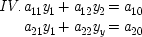
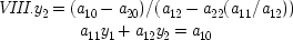
Consider identifiability first. In the completely deterministic case under consideration here, where the us represent real properties, probabilities never need to enter. The relevant observational facts are about individuals and what values they take for the variables x 1. . . , x e. Each individual, i, will provide a set of values {x 1i, . . . , x ei}. Can the parameters a e1, . . . , a ee− 1, be determined from data like that? The answer is familiar from elementary algebra. It will take observations on e − 1 individuals, but that is enough to identify all e − 1 parameters, so long as the variables themselves are not linearly dependent on each other.
A simple three-dimensional example will illustrate.
Given the values {
o 1,
o 2,
o 3} for the first observation of
x 1,
x 2, and
x 3, and {
p 1,
p 2,
p 3} for the second, two equations result
Solving for
a and
b gives
Imagine, though, that
x 1and
x 2are linearly dependent of each other, i.e.
x 1= Γ
x 2for some Γ. Then
p 1= Γ
p 2and
o 1= Γ
o 2, which
end p.30
implies that p 1o 2= p 2o 1. So the denominators in the equations for a and b are zero, and the two parameters cannot be identified. Because x 1and x 2are multiples of each other, there is no unique way to partition the linear dependence of x 3on x 1and x 2into contributions from x 1and x 2separately; and hence no sense is to be made of the question whether the coefficient of x 1or of x 2is 'really' zero or not. This result is in general true. All e − 1 parameters in the equation for x ecan be identified from e − 1 observations so long as none of the variables is a linear combination of the others. If some of the variables are linearly related, no amount of observation will determine all the parameters.
These elementary facts about identifiability are familiar truths in econometrics and in modelling theory. What is not clearly agreed on is the connection with causality, and the remarkable fact that the very same condition that ensures the identifiability of the parameters in an equation like that for x ealso ensures that the equation can be given its natural causal reading—so long as a generalized version of Reichenbach's principle of the common cause can be assumed. The argument is exactly analogous with that for inus causes. If the factors with non-zero coefficients on the right-hand side of the equation for x eare all true causes of x e, everything is fine. But if not, how does that equation come to be true? Reichenbach's principle, when generalized, requires that every true functional relationship have a causal account. In the context of linear modelling theory, this means that any equation that does not itself represent true causal relations must be derivable from equations that do. So if the equation contains spurious causes, it must be possible to derive it from a set of true causal equations, recursive in form, like those at the beginning of this section. But if each of the equations of the triangular array contains a u that appears in no other equation, including the spurious equation for x e, this will clearly be impossible. The presence of the us in the preceding equations guarantees that the equation for x emust give the genuine causes. Otherwise it could not be true at all.
This argument can be more carefully put as a small theorem. The theorem depends on the assumption that each of the xs on the right-hand side of an equation like that for x esatisfies something that I will call the 'open back path requirement'. For convenience of expression, call any set of variables that appear on the right-hand side of a linear equation for x ea 'full set of inus conditions' for x e, by analogy
end p.31
with Mackie's formulae. Only full sets where every member could be a cause of x e, so far as we know, need be considered. Recall that the variables under discussion are supposed to be time-indexed, so that this requires at least that all members of the full set represent quantities that obtain before x e. But it also requires that there be nothing else in our background assumptions to rule out any of the inus conditions as a true cause.
The open back path assumption is analogous with the assumption that was made about the Manchester timekeeper: every inus condition in the set must have at least one cause that is known not to be a cause of x e, and each of these causes in turn must have at least one cause that is also known not to be a cause of x e, and so forth. The second part of the condition, on causes of causes, was not mentioned in the discussion of Mackie's example, but it is required there as well. It is called the 'open back path condition' (OBP) because it requires that at any time-slice there should be a node for each inus factor which begins a path ending in that factor, and from which no descending path can be traced to any other factor which either causes x e, or might cause x e, for all we know. This means not only that no path should be traceable to genuine causes of x e, but also that none should be traceable to any of the other members of the full set under consideration. The condition corresponds to the idea expressed earlier that every inus condition x should have at least one causal history which is known not to be able to cause x eindependently, but could do so, if at all, only by causing x itself.
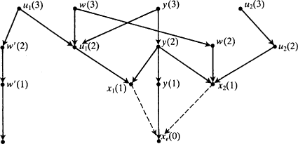
Fig.
1.4 gives one illustration of this general structure. The inus conditions under consideration are labelled by
xs; true causes by
ys;
end p.32
factors along back causal paths by us; and other factors by ws. Time indices follow variables in parentheses. In the diagram u 1(3). u 1(2) forms an open back path for x 1(1); and u 2(3). u 2(2), for x 2(1). The path y(3). u 1(2) will not serve as an open back path for x 1(1), since y(3) is a genuine cause, via y(2), of x e(0), and hence cannot be known not to be. Nor will w(3). u 1(2) do either, since w(2) causes x 2(0), and hence may well, for all we know, have an independent route by which to cause x e(0).
Notice that these constructions assume the transitivity of causality: if y(2) causes y(1) which causes x e(0), then y(2) causes x e(0) as well. This seems a reasonable assumption in cases like these where durations are arbitrary and any cause may be seen either as an immediate or as a more distant cause, mediated by others, depending on the size of the time-chunks. The transitivity assumption is also required in the proof of the theorem, where it is used in two ways: first in the assumption that any x which causes a y is indeed a genuine cause itself, albeit a distant one by the time-chunking assumed; and second, to argue, as above, that factors like w(2) that cause other factors which might, so far as we know, cause x e(0) must themselves be counted as epistemically possible causes of x e(0).
The theorem which connects inus conditions with causes is this:
If each of the members of a full set of inus conditions for x emay (epistemically) be a genuine cause of x e, and if each has an open back path with respect to x e, all the members of the set are genuine causes of x e
where
OBP: x(t) has an open back path with respect to x e(0) just in case at any earlier time t′, there is some cause, u(t′), of x(t), and it is both true, and known to be true, that u(t′) can cause x e(0) only by causing x(t).
The theorem is established in the appendix to this chapter. It is to be remembered that the context for the theorem is linear modelling theory, so it is supposed that there is a linear equation of the appropriate sort corresponding to every full set of inus conditions. What the appendix shows is that if each of the variables in an equation for x ehas an open back path, there is no possible set of genuine causal equations from which that equation can be derived, save itself. Reichenbach's idea must be added to complete the proof. If every true equation must either itself be genuinely causal, or be derivable from other equations that are, then every full set of inus conditions with open back paths will be a set of genuine causes.
end p.33
It may seem that an argument like that in the appendix is unnecessary, and that it is already apparent from the structure of the equations that they cannot be transformed into an equation for
x ewithout introducing an unwanted
u. But the equations that begin this section are not the only ones available. They lay out only the causes for the possibly spurious variables
x 1,
x 2, . . . ,
x e − 1. Causal equations for the genuine causes—call them
y 1, . . . ,
y m—will surely play a role too, as well as equations for other variables that ultimately depend on the
xs and
ys, or vice versa. All of these equations can indeed be put into a triangular array, but only the equations for the
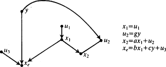
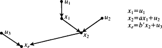
xs will explicitly include
us. A simple example will illustrate. Fig.
1.5(a) gives the true causal structure, reflected in the accompanying equations; Fig.
1.5(b) gives an erroneous causal structure, read from its accompanying equations, which can be easily derived from the 'true' equations of Fig.
1.5(a). So it seems that we need the slightly more cumbersome argument after all.
1.5. Conclusion
This chapter has tried to show that, contrary to the views of a number of pessimistic statisticians and philosophers, you can get
end p.34
from probabilities to causes after all. Not always, not even usually—but in just the right circumstances and with just the right kind of starting information, it is in principle possible. The arguments of this chapter were meant to establish that the inference from probability to cause can have the requisite bootstrap structure: given the background information, the desired causal conclusions will follow deductively from the probabilities. In the language of the Introduction, probabilities can measure causes; they can serve as a perfectly reliable instrument.
My aim in this argument has been to make causes acceptable to those who demand a stringent empiricism in the practice of science. Yet I should be more candid. A measurement should take you from data to conclusions, but probabilities are no kind of data. Finite frequencies in real populations are data; probabilities are rather a kind of ideal or theoretical representation. One might try to defend probabilities as a good empirical starting-point by remarking that there are no such things as raw data. The input for any scientific inference must always come interpreted in some way or another, and probabilities are no more nor less theory-laden than any other concepts we use in the description of nature. I agree with the first half of this answer and in general I have no quarrel with using theoretical language as a direct description of the empirical world. My suspicion is connected with a project that lies beyond the end of this book. Yet it colours the arguments throughout, so I think it should be explained at the beginning.
The kinds of probability that are being connected with causality in this chapter and in later chapters, and that have indeed been so connected in much of the literature on probabilistic causality over the last twenty years, are probabilities that figure in laws of regular association. They are the non-deterministic analogue of the equations of physics; and they might be compared (as I have done) to the regularities of Hume: Hume required uniform association, but nowadays we settle for something less. But they are in an important sense different from Hume's regularities. For probabilities are modal
30or nomological and Hume's regularities were not. We nowadays take for granted the difference between a nomological and an accidental generalization: 'All electrons have mass' is to be distinguished from
end p.35