3. Basic components and methods
Population viability analysis (PVA) is the use of quantitative models to predict future population growth and extinction risks. PVA includes a variety of methods to gauge the sensitivity of population viability to natural and human-caused impacts and to estimate the efficacy of management interventions in promoting population growth and safety from extinction. PVA began as a field that borrowed tools from basic population ecology and applied them to conservation questions. From those beginnings, PVA has matured into a discipline that drives innovations in analysis methods and tries more generally to address the processes of conservation planning and priority setting. Because of their wide usage, in particular for assessing management actions, PVA approaches have been closely scrutinized, and the field continues to refine its methods to tackle key criticisms. In summary, PVA has provided specific guidance that has aided the recovery of scores of endangered species and has helped to crystallize several general principles in conservation.
demographic stochasticity. Unpredictability through time in a population’s demography (how many individuals die, how many reproduce, etc.) caused by the randomness of individual fates. This type of stochasticity is usually important only at very small population sizes.
environmental stochasticity. Unpredictable changes through time in average demographic rates of a population. These changes can be caused by vacillations in weather, food, predators, or other biotic and abiotic forces influencing individuals in a population and can exert strong effects on the dynamics of populations.
genetic stochasticity. Unpredictable changes in gene frequencies as a result of processes such as random genetic drift. This type of stochasticity is usually important only at very small population sizes.
inbreeding depression. The decline in measures of individual performance (e.g., survival, growth, or reproduction) sometimes seen in offspring of parents that are closely related to one another.
lambda(λ). Annual population growth rate.
metapopulation. In general, a collection of populations that are connected by movement. More specifically, the term is usually reserved for a collection of populations each of which has reasonably high probabilities of local extinction and also of recolonization.
Nt. Population size in year t.
parameters. Values used to describe population dynamics in models, such as the mean or variance in fecundity or survival rate.
population viability. The probability of continued existence of a population. Viability is the converse of the risk of extinction (often defined in terms of quasiextinction rather than complete extinction) over some time period.
quasiextinction threshold (Nqe). The minimum number of individuals below which a population is likely to be critically and immediately imperiled.
The International Union for Conservation of Nature (IUCN) currently recognizes over 15,000 species as threatened with extinction worldwide (http://www.iucnredlist.org/). However, given the uncertainty surrounding the status of numerous species or even how many species exist, the number of imperiled species on a global scale is almost certainly considerably more than those documented by the IUCN. The causes of species endangerment vary (see chapter V.1), but in all cases, conservation biologists working to avert extinctions wish to understand the degree of risk facing a particular species or population. Even more importantly, they wish to identify practical management actions that can substantially improve the viability—the long-term chances of persistence—of threatened populations. To answer these questions, the discipline of population viability analysis (PVA) has emerged over the last three decades. PVA, defined broadly, is the use of quantitative methods to predict the likely future status of populations of conservation concern and also to predict how best to manage these populations.
PVA grew into a distinct field in ecology because making predictions about population persistence is quite difficult. As Yogi Berra once said (perhaps misquoting a similar observation by Niels Bohr), “It’s tough to make predictions, especially about the future,” and this is particularly true for the population processes described in PVAs, which are typically known only through imperfect data and are influenced by myriad random, or stochastic, forces. PVAs are developed to generate these hard-to-make predictions in a way that is clearly reasoned and quantitative rather than based solely on expert opinion. Importantly, constructing a quantitative PVA model requires explicit articulation of what is known about a population versus what is assumed or guessed. Thus, the process of conducting a PVA hones a management team’s thinking about conservation problems and data limitations while providing better and more defensible answers. Although critics of PVAs have sometimes taken aim at the accuracy of PVA predictions, there is general agreement that comparing the predictions of a PVA for one management scenario relative to another usually provides robust and useful guidance for decision makers.
PVAs have utility in a wide variety of management and basic ecological contexts. Over the years they have been used to answer such questions as: (1) What life stages should be prioritized for increased protection in order to decrease short-term extinction risks of a rare population? (2) How large do reserves need to be in order to maintain key species? (3) What parts of the life cycle should be targeted to reduce or eliminate populations of invasive species? (4) How can the harvest of populations be maximized without causing declines? (5) What features of metapopulations will allow them to persist in patches of fragmented habitat? New directions in the field include integrating PVA more directly into adaptive management decisions, evaluating the effects of sublethal threats on population persistence, and predicting the effects of multispecies interactions on extinction risks.
As of this writing, PVAs number in the hundreds to thousands and range from analyses for tiny fairy shrimp confined to vernal pools to those for whale populations spanning entire oceans. In spite of this diversity, PVAs generally share the same basic components. All PVAs are descriptions of the dynamics of a population or a collection of populations. As such, almost any population model could be considered a PVA, especially if it is used to describe imperiled or managed populations (see chapters II.1, II.2, and II.4 for basic discussions of population models). PVA first emerged as a distinct discipline within population ecology with Mark L. Shaffer’s 1978 analysis of the Yellowstone grizzly population. Shaffer built a demographic model for this isolated bear population and used computer simulations to estimate the numbers of bears needed to ensure a reasonable chance (Shaffer chose 95%) of persistence over the next 100 years. By providing a mathematical description of how this population worked—the deterministic and stochastic processes that made numbers grow or shrink through time—and using it to ask about future viability under different scenarios of management, initial numbers, and other factors, Shaffer’s analysis established many of the features that still characterize PVAs today.
Since Shaffer’s first PVA, over 25 PVAs have been published for grizzlies, with at least 18 different models for the Yellowstone population alone. This great number of PVAs, including new and distinct PVAs for the same population, reflect both the usefulness of PVA results to management and the evolution of scientific understanding about the critical forces impacting populations. For example, during the 1980s, key concerns in many PVAs were loss of genetic variation and the resulting processes of inbreeding and inbreeding depression. However, faced with continued ignorance of how genetic inbreeding influences survival and reproduction, developers of PVAs have since shifted away from explicit consideration of genetics, focusing instead on maintaining populations at large enough numbers that loss of genetic diversity and inbreeding depression are unlikely to be serious problems. This minimum acceptable size, defined in part by genetic factors, is referred to as a quasiextinction threshold. In the 1990s, and continuing to the present, PVAs have typically concentrated on the impacts of environmental stochasticity, human-caused threats, and the spatial dynamics of metapopulations. Most recently, PVAs have begun to account for climate change and invasive species impacts because of the increased importance of these threats to population survival. These trends in the conditions and complications that PVAs emphasize reflect a key feature of this field of conservation biology: PVA methods are applied to rare species in dynamic systems for which conservation biologists generally possess incomplete knowledge of both population processes and current and future threats. Indeed, one criticism of PVAs is that they cannot account for unforeseen changing future conditions, and thus, many scientists advocate their use only for relatively short time horizons. In addition to restricting time horizons, PVA predictions can be improved by periodically refining models as methods improve, understanding of parameter values increases, or ecological systems change.
The most important rule of constructing a PVA is to keep it simple. Although it is tempting to include every possible ecological effect in modeling a population, the most robust PVA models are generally those that are less complex, based on reliable data, and tailored to fit what is known rather than simply guessed. For example, although the impacts of invasive species on a threatened plant might be expected to increase over the next 50 years, with no information on how fast or how much these impacts will change, it may be better to leave out this “realism” and instead clearly note that assuming current impact levels is optimistic. Even though the complexity of PVA models should be limited to fit the available data, some key ecological processes are almost always considered. These are outlined below along with a description of the basic model forms and useful outputs of many PVAs.
PVA models can be divided into two main categories: deterministic and stochastic. Deterministic models are simple projections of population growth rate and future population sizes without consideration of the variability in model parameters from year to year. As such, deterministic models are of limited value in predicting longer-term population numbers or viability and instead are used to compare the general efficacy of different management strategies for populations with limited data. In contrast, stochastic models incorporate estimates of temporal variability in demographic rates or the overall population growth rate to better represent the “real world.” Adding stochasticity to a model generally increases the estimated risk of extinction because otherwise healthy populations may experience a series of bad years by random chance. Models can include either environmental or demographic stochasticity or, frequently, both. Less frequently, models will also incorporate genetic influences, such as genetic stochasticity (i.e., random genetic drift) and inbreeding depression. As noted earlier, detailed information on the impacts of inbreeding on individual fitness of wild species is rarely available, so explicit treatment of genetic stochasticity is now uncommon in PVAs.
Environmental stochasticity is randomness in demographic rates (e.g., birth, growth, and survival rates) caused by environmental factors such as weather. Extreme forms of environmental stochasticity occur as rare years of extraordinarily good or bad conditions, which are frequently of greater importance for viability than less extreme but more frequent year-to-year variations. Demographic stochasticity is variation created by chance differences in the fates of individuals, such as the random possibility that 10 members of a population of 20 will die in a particular year, even though the true mean annual survival rate is 80%. Demographic stochasticity is considered less of a threat to population persistence than environmental stochasticity, and its influence is felt only at small population sizes (i.e., ~50). Nonetheless, demographic stochasticity causes populations to grow more slowly and erratically at low numbers, making predictions of complete extinction more difficult than predictions of declines to a very low population size. As with genetic stochasticity and inbreeding depression, using a quasiextinction threshold allows PVAs to account for the diminished ability to predict the fates of very small populations due to demographic stochasticity.
Adequately characterizing the effects of environmental stochasticity also requires consideration of correlations in the different effects of environmental variables. The environment often, but not always, affects many life stages similarly. For example, severe winters may reduce survival rates at all ages and also depress reproduction the following spring. Likewise, some environmental factors, such as droughts, tend to persist for several years, causing demographic rates to be similar from one year to the next, producing autocorrelation in rates through time. Finally, populations in close proximity to each other are apt to experience similar environmental conditions at the same time, or spatial autocorrelation. In general, positive correlations in demographic rates, in either time or space, tend to reduce population viability, and hence are of concern for conservation planning.
To simulate competition for limited resources, many PVAs impose negative density dependence, such that population growth rates decline as populations grow, or they impose a cap on the population size at the estimated carrying capacity. PVAs can model negative density dependence in many different ways, and results are quite sensitive to the specific approach used (see chapter II.3 for further discussion of this issue in population modeling). This sensitivity, along with a scarcity of field data clearly demonstrating the presence and form of negative density dependence for many rare species, means that great care is needed in deciding whether and how to include it in a PVA. Another theoretical possibility, but one also lacking strong empirical support in most situations, is the presence of Allee effects, or positive density dependence at low densities, such that population growth rates drop when densities are sparse because of the disruption of social interactions. For example, animals that rely on group dynamics to hunt or defend themselves, such as wolves or musk oxen, are likely to have reduced survival rates once their group size falls below a certain threshold. Although Allee effects will always increase extinction risk, they are thought to operate primarily at very low densities and are often accounted for by use of a quasiextinction threshold.
Most PVAs are built around one of four general types of population models:
Count- or Census-Based Models
These PVAs predict future population numbers and viability using mean annual population growth rate (λ) estimated from multiple counts of total population size (or a proxy for total population size) over a specific time period and incorporate environmental stochasticity through variance in λ. At their most basic, these models take the form:
where Nt is the number of individuals at time t, and λt is the population growth rate at time t. The growth rate over 1 year can be calculated from two annual counts as λt = Nt+1/Nt. The mean and variance of the natural logarithms of these λt values are typically used to characterize stochastic growth rates. Count-based PVAs are a direct extension of the simplest descriptions of population growth, such as exponential growth (equation 1) or slightly more complex model forms that impose a ceiling on total population size or incorporate negative density dependence in growth rates. Examples of these more complex model forms are the Ricker equation, first developed for fisheries management, or the logistic growth equation, both of which impose lower and lower growth rates as the size of a population approaches its carrying capacity (see chapters II.1 and II.2).
Demographic Models
Historically, the majority of PVAs have used life tables or population matrix models built with demographic rates (e.g., survival and reproductive rates) to describe population dynamics. These models take different forms depending on whether individuals are classified by age, life stage (e.g., larvae versus adults), or size classes. To understand the basic form of a matrix model, it is helpful to think of a simple example, such as a population that is censused in the spring just after offspring are born and consists of three age groups, or stages: newborns, 1-year-olds, and all older adults. A simple demographic model for the female part of this population (almost all demographic models track only females) uses methods from linear algebra to multiply a matrix of demographic rates (A) by a vector containing the number of individuals in each stage (B) to obtain numbers in each age class the following year (C) (also see chapter II.1):
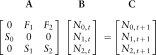
In this equation, the Ni, t terms indicate numbers of individuals of stage i at time t. The Si elements in the matrix are annual stage-specific survival probabilities. The Fi elements are slightly trickier, as they delineate the stage-specific reproductive output for each individual over a 1-year period. For example, F2 is the average number of newborns (stage 0 individuals) produced a year from now by each older adult individual (stage 2 individual) we see now. Thus, F2 is actually composed of two parts: the probability that an adult female we see now survives for a year multiplied by the number of female offspring she will produce if she does survive. Demographic PVAs often include environmental and demographic stochasticity through computer simulation of variation in one or more demographic rates. These models offer an advantage over count- or census-based models because they can be used to directly assess the effects of threats, harvest, or management interventions targeting particular stages or demographic rates (see example 1 below).
Metapopulation and Spatially Structured Models
This category of PVA includes several types of population representations but always emphasizes a collection of distinct populations linked by movement (see chapter II.4). Spatial models may simply estimate the proportion of available sites occupied by the species of interest, based on extinction and colonization rates, or they may consist of complex matrices accounting for site-specific survival and reproductive rates as well as intersite movement rates. Their key advantage is the ability to predict overall population persistence when local groups of individuals are growing and disappearing over time as well as to distinguish the fates of different (yet linked) populations, some of which are likely to occupy better or worse habitat (see example 2 below).
Individually Based Simulation Models
Like the last type of PVA, models in this category include a range of population representations, but all rely on extensive computer simulations to track the fates and locations of individuals. They are usually used for animals and tend to emphasize the importance of individual movements and location, and thus, they are a special form of spatially structured PVA. Although these are the most data-hungry form of PVA, they also allow the tightest links with habitat and behavior, which may interact to influence population viability (see example 2 below).
Again, the type of PVA model chosen should depend on the data available to build it. For example, census-based PVAs are appropriate for species for which monitoring programs have collected count data over many years (such as many African ungulates and North American breeding bird species). At the other extreme, if detailed annual data exist for the survival, reproduction, and movements of many marked individuals, an individually based simulation may be advantageous.
Once a PVA model is constructed, it can be analyzed in various ways to yield valuable information about how threatened a population is and what management methods have the greatest chance to increase viability. The most important of these outputs are the following.
Expected Growth Rates
The most basic and often the most useful output of a PVA is the population’s current annual growth rate, or λ. For deterministic models, the single estimate of mean growth rate will predict whether the modeled population is increasing (λ>1), stable (λ=1), or decreasing (λ<1). In contrast, stochastic models predict not only a mean λ but also a range of possible growth rates, reflecting our uncertainty about the particular series of future environmental conditions that may occur. Critically, by ignoring variability in population performance, a predicted λ from a deterministic model will likely overestimate the long-term growth of real-world populations. Further, even if the average λ for a stochastic model is greater than 1, a population can still by chance decline or become extinct.
Future Population Size
PVAs also predict the probabilities of different future population sizes. This output is important to evaluate such things as average number of years to extinction or the probability of extinction in a specified time frame for the population of interest. Furthermore, if a recovery program is initiated, a PVA can provide managers with a prediction of how long it will take for the population to reach a target number or density.
Extinction Risk
PVAs can assess the extinction risk of a single population or compare the relative risks of two or more different populations. These risks usually evaluate the probability that a population will decline to a quasiextinction threshold within a certain time horizon (e.g., 50 years).
Sensitivity
Sensitivity values (and the related elasticity values) determine which parameters in a model have the greatest influence on λ by observing the degree of change in λ relative to a change in an individual model parameter (e.g., adult survival). Sensitivity results can also be estimated for extinction risk or other outputs of a PVA. The results of sensitivity analysis help prioritize different conservation and management efforts, such that the most sensitive stage or age class of a population is targeted for management efforts (see example 1 below). For example, sensitivity analyses have clarified the disproportionate value of older individuals relative to young of the year for essentially all long-lived, late-maturing species, which are over-represented in the ranks of endangered species lists worldwide.
Loggerhead sea turtles (Caretta caretta) are threatened marine turtles that breed on coastal beaches and feed as juveniles and adults, in part, on pelagic and nearshore invertebrates. Two prominent threats related to these life-history characteristics are (1) loss and degradation of nesting habitat and direct harm to eggs and hatchlings, and (2) drowning of individuals in the nets of fishing boats trawling for shrimp. Despite a long-term decline in loggerheads, there was debate in the 1980s about where to focus conservation efforts, with the greatest momentum in protecting nesting habitat and individual nest sites. To understand which of these efforts was most useful in stabilizing turtle numbers, in 1987 Deborah T. Crouse and her associates constructed a demographic PVA and performed a sensitivity analysis. They demonstrated that survival of all older age classes, especially large juvenile turtles, had a much greater effect on λ than the survival of turtle eggs (plate 15, inset). This was perhaps the most influential use of sensitivity analysis in any PVA. This analysis and subsequent work led to the installation of turtle excluder devices (TEDs) on shrimp trawlers in nearshore waters of the southeastern United States by 1994. TEDs allow most large turtles caught in nets to escape unharmed (plate 15), and use of these devices has spread to other fisheries to protect other sea turtle populations and has spawned the innovation of additional measures to reduce marine by-catch.
Perhaps the best known spatial PVAs emerged during the intense scrutiny of forest management plans for the northern spotted owl (Strix occidentalis caurina) in the 1980s. Conservation biologists built a range of PVAs that incorporated the spatial structure of territories and the movement of juveniles between them to find vacancies within these territories. These models ranged from the initial, elegantly simple analysis of Russell Lande in 1988 that assumed general rules of movement and landscape configuration to intensive simulations of individual owls and realistic landscapes. Importantly, these different PVAs all showed that owl populations had little chance of survival without drastically altered forest management practices and, in particular, showed the need for regeneration of large blocks of habitat that were not fragmented by logging operations.
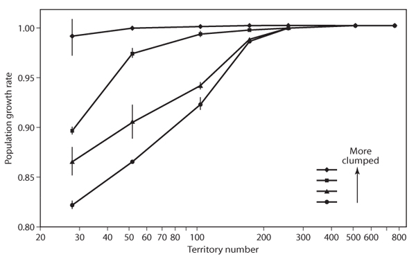
Spatial modeling is frequently hampered by a lack of data on movement, but when data are available, spatial PVAs offer very useful results. A decade after Lande published his spatial model on spotted owls, Benjamin H. Letcher and colleagues used detailed data on dispersal distances to develop an individually based, spatially explicit PVA for the threatened red-cockaded woodpecker. They concluded that protecting forest patches containing aggregated territories led to much higher population persistence than the same number of dispersed territories (figure 1), a very similar result to that of the northern spotted owl PVAs.
Although PVAs have dramatically increased in sophistication, most analyses do only a cursory job of analyzing the complexities of human management and monitoring activities and instead concentrate on the details of ecology. Island foxes (Urocyon littoralis) are endemic to six of the Channel Islands, located off the coast of southern California. Populations plummeted on four of the islands in the 1990s as a result of predation by golden eagles and a disease epidemic, propelling the island fox onto the endangered species list. For this species to persist, expensive and complicated management activities will be needed for the foreseeable future. Thus, a PVA that analyzes the details of these human actions, as well as ecological processes, is required. Two of us (D.F.D. and V.J.B.) built a demographic PVA for the fox that accounted for both data uncertainties and the strong density dependence observed in survival rates (plate 16). The model predicts rapidly increasing risk of extinction with the addition of eagle predation. Sensitivity analysis for this model also shows that adult survival is the most important life stage to manage for—but this result did not provide guidance on how best to manage threats to adult survival given available resources. To advise managers on how to use their resources to keep eagle predation, and hence risk of extinction, to acceptable levels, we simulated different levels of eagle control (capture and removal) as well as different intensities of fox mortality monitoring (the data used to decide when to start and stop eagle control). This model, along with similar models we built to assess disease risk abatement strategies, and alternative monitoring approaches, are unusual in that they simulate the managers and their actions as well as foxes and their biology, thus linking different levels of monitoring and management effort directly to estimated extinction risk (plate 16, bottom panels).
Figure 1. Population growth rate of the red-cockaded woodpecker as a function of territory number and degree of aggregation (clumping) of territories. Symbols represent growth rates in landscapes where territories have different levels of aggregation, circles being the least clumped and diamonds being the most. The same number of territories produced a higher population growth rate if the territories were aggregated than if they were randomly spaced. (Figure from Letcher et al., 1998)
Scientists will continue to advance their understanding of what threats and complications are pivotal to assessments of population viability and how these should best be included in PVAs. Additional changes in the thrust of PVAs will be motivated by ever-changing global and local conditions. For example, climate change is predicted to accelerate over the coming decades, while in some (but not all) parts of the world, poaching is declining. Three processes or threats that are receiving increased attention in PVAs are (1) the health effects of toxic substances, (2) movement and spatial effects, and (3) species interactions. These factors may be fruitfully incorporated within PVAs as more and better research methods allow clearer characterization of these complex issues.
Traditionally, PVAs account for direct mortalities from sources such as hunting, habitat destruction, and predation, but not the effects of sublethal threats such as contaminant exposure and disease, which may slowly or indirectly impair survival, reproduction, and growth. For example, blackfooted albatrosses are large pelagic seabirds that forage over entire ocean basins. These birds are exposed to very high concentrations of organochlorine contaminants such as PCBs and DDT, and there is mounting evidence that they suffer sublethal effects from these contaminants. Although accidental mortality from fishing practices is currently thought to be the biggest threat to black-footed albatross population viability, incorporating sublethal effects of contaminant exposure into PVAs for these and related birds will allow for a more comprehensive prioritization of conservation efforts.
Although many PVAs have incorporated spatial processes (example 2), including metapopulation and source–sink population dynamics, better information about how animals respond to habitat fragmentation and make movement decisions is broadening the range of spatial complexities that PVAs can include. In particular, the advent of GPS radiocollars for wideranging animals, micro-radiotags for small species, implantable sonic tags for fish, and pop-off tags for pelagic marine species heralds unprecedented gains in understanding how animals use complex habitats and how this use influences their birth, death, and growth rates. These advances in tracking technology may inject new vigor into spatial PVA modeling, and in particular, to individually based simulation models.
A final area in which PVAs are expanding is the consideration of species interactions within PVA models. Although PVAs are virtually always focused on single species, many of the forces influencing any one population are the co-occurring populations of predators, prey, or competitors. Many PVAs do include the effects of predators, prey, or humans on the focal population. Nonetheless, the way that this is done is usually static, without a full consideration of the dynamics of these interacting populations. Increasingly, there are efforts to consider how the fuller dynamics of species interactions can be incorporated into PVAs.
PVAs typically focus on the biology of the population being analyzed. Although not inherently unreasonable, this means that most PVAs ignore the human foibles that influence both the development of models and the carrying out of management plans. First, although the data used to build PVAs are always incomplete and imperfect, most have not tried to incorporate this uncertainty into their predictions. Thus, a major criticism of past PVAs is that they fail to account for parameter uncertainty, and in particular that they are interpreted as if their mathematical depictions of a species’ biology were perfect. Solving this problem can be mathematically complex and computationally difficult, but recent PVAs have begun to take the problem of data uncertainty seriously. The resulting analyses are more robust and can also be used to analyze which data gaps most limit our ability to make powerful predictions about endangerment and management of sensitive populations. The second problem that PVAs are now tackling is the intricacy of monitoring and management programs, which themselves require careful decisions and can never be perfectly implemented. Although standard sensitivity analyses give important general answers about how best to manage, more explicit simulation of specific management actions—and ongoing data collection—allows better tailoring of PVA recommendations to real issues for endangered species managers (see example 3).
PVAs have become powerful tools for conservation biology that help to evaluate the risk of extinction for different populations and to guide management in ways that improve conservation efforts. One could, nonetheless, ask why conservation biologists should put so much effort into detailed analyses of single species when conservation is—or at least is argued to be—mostly concerned with multispecies communities and entire ecosystems. This is a fair question, but both biological and political realities make PVA an essential tool for today’s conservation challenges. First, there is no “endangered community act,” but the IUCN, the Endangered Species Act of the United States, and similar legislation in other countries do provide protection for endangered populations and species. Thus, PVA dovetails with the conservation laws we actually have. Second, although evaluating the risk of extinction can involve complex analyses, the biological reality being estimated—the risk of extinction of a population—is crystal clear. There is no correspondingly clear or biologically relevant standard of “community viability” or “community extinction.” For example, communities can be highly altered without suffering any population extinctions, and conversely, communities and ecosystems may appear largely unaltered despite the extirpation of some formerly present species. Thus, even when we are concerned with the viability of a community, conducting PVAs for keystone and umbrella species may provide one of the strongest and most defensible ways to evaluate conservation risks.
Given these considerations, PVA is likely to remain a strong branch of ecology and conservation for the foreseeable future. Already we are seeing novel applications of PVA methods to reserve design, invasive species management, and other branches of conservation that are discussed in the following chapters.
Crouse, D., L. Crowder, and H. Caswell. 1987. A stage-based population model for loggerhead sea turtles and implications for conservation. Ecology 68: 1412–1423.
Lande, R. 1988. Demographic models of the northern spotted owl (Strix occidentalis caurina). Oecologia 75: 601–607.
Letcher, B. H., J. A. Priddy, J. R. Walters, and L. B. Crowder. 1998. An individual-based, spatially-explicit simulation model of the population dynamics of the endangered red-cockaded woodpecker, Picoides borealis. Biological Conservation 86: 1–14.
Shaffer, M. L., and F. B. Sampson. 1985. Population size and extinction: A note on determining critical population size. American Naturalist 125: 144–152.
Mills, L. S. 2006. Conservation of Wildlife Populations: Demography, Genetics, and Management. New York: Blackwell Publishing.
Morris, W. F., and D. F. Doak. 2002. Quantitative Conservation Biology: The Theory and Practice of Population Viability Analysis. Sunderland, MA: Sinauer Associates.