
The theory of investments is based on the premise that assets are fairly valued. This is reassuring for the financial economist and frustrating to the active manager. The active manager needs theoretical support. In the next four chapters we will provide a structure, if not a theory, for the active manager.
This chapter starts the process by building a strategic context for management of residual risk and return. Within that context, we will develop some concepts and rules of thumb that we find valuable in the evaluation and implementation of active strategies.
The reader is urged to rise above the details. Do not worry about transactions costs, restrictions on holdings, liquidity, short sales, or the source of the alphas. We will deal with those questions in later chapters. At this point, we should free ourselves from the clutter and look at active management from a strategic perspective. Later chapters on implementation will focus on the details and indicate how we might adjust our conclusions to take these important practical matters into consideration.
There is no prior theory. We must pull ourselves up by our bootstraps. Economists are good at this. Recall the parable of the engineer, the philosopher, and the economist stranded on a South Sea island with no tools, very little to eat on the island, and a large quantity of canned food. The engineer devises schemes for opening the cans by boiling them, dropping them on the rocks, etc. The philosopher ponders the trifling nature of food and the ultimate futility of life. The economist just sits and gazes out to sea. Suddenly, he jumps up and shouts, “I’ve got it! Assume you have a can opener.”
The active manager’s can opener is the assumption of success. The notion of success is captured and quantified by the information ratio. The information ratio says how good you think you are. The assumption of future success is used to open up other questions. If our insights are superior to those of other investors, then how we should use those insights?
We proceed with can opener and analysis. The results are insights, rules of thumb, and a formal procedure for managing residual risk and return. Some of the highlights are:
■ The information ratio measures achievement ex post (looking backward) and connotes opportunity ex ante (looking forward).
■ The information ratio defines the residual frontier, the opportunities available to the active manager.
■ Each manager’s information ratio and residual risk aversion determine his or her level of aggressiveness (residual risk).
■ Intuition can lead to reasonable values for the information ratio and residual risk aversion.
■ Value added depends on the manager’s opportunities and aggressiveness.
The chapter starts with the definition of the information ratio, which is one of the book’s central characters. In this chapter we use the information ratio in its ex ante (hope springs eternal) form. The ex ante information ratio is an indication of the opportunities available to the active manager; it determines the residual frontier. In Chap. 4 we defined an objective for the active manager that considers both risk and return. The main results of this chapter flow from the interaction of our opportunities (information ratio) with our objectives.
In Chap. 4 we showed that a manager could add value through either benchmark timing or stock selection. We postpone the discussion of benchmark timing to Chap. 19 and will concentrate on stock selection until that point. This means that we are concerned about the trade-off between residual risk and alpha. Recall that when portfolio beta is equal to 1, residual risk and active risk coincide.
A technical appendix considers the information ratio in merciless detail.
Looking forward (ex ante), alpha is a forecast of residual return. Looking backward (ex post), alpha is the average of the realized residual returns.
The term alpha, like the term beta, arises from the use of linear regression to break the return on a portfolio into a component that is perfectly correlated with the benchmark and an uncorrelated or residual component. If rP(t) are portfolio excess returns in periods t = 1,2, ... T and rB(t) are benchmark excess returns over those same periods, then the regression is
The estimates of βP and αP obtained from the regression are the realized or historical beta and alpha. The residual returns for portfolio P are
where αP is the average residual return and ∈P(t) is the mean zero random component of residual return.
This chapter concentrates on forecast alphas. In Chap. 12, “Information Analysis,” we’ll learn how to evaluate the quality of the alpha forecasts. We’ll consider realized alphas in Chap. 17, “Performance Analysis.” Realized alphas are for keeping score. The job of the active manager is to score. To do that, we need good forecast alphas.
When we are looking to the future, alpha is a forecast of residual return. Let θn be the residual return on stock n. We have
Alpha has the portfolio property, since both residual returns and expectations have the portfolio property. Consider a simple case with two stocks whose alphas are α1 and α2. If we have a two-stock portfolio with holdings hP(1) in stock 1 and hP(2) in stock 2, then the alpha of the portfolio will be
This is consistent with the notion that αP is the forecast of expected residual return on the portfolio.
By definition, the benchmark portfolio will always have a residual return equal to 0; i.e., θB = 0 with certainty. Therefore, the alpha of the benchmark portfolio must be 0; αB = 0. The requirement that αB = 0 is the restriction that the alphas be benchmark-neutral.
Recall that the risk-free portfolio also has a zero residual return, and so the alpha for cash αF is always equal to 0. Thus any portfolio made up of a mixture of the benchmark and cash will have a zero alpha.
An information ratio,1 denoted IR, is a ratio of (annualized) residual return to (annualized) residual risk. If we consider the information ratio for some realized residual return (ex post), we have realized residual return divided by the residual risk taken to obtain that return. Thus we may have an average of 2.3 percent residual return per year with residual risk of 3.45 percent. That is an information ratio of 2.3/3.45 = 0.67.
A realized information ratio can (and frequently will) be negative. Don’t forget that the information ratio of the benchmark must be exactly zero. If our residual return has averaged a poor —1.7 percent per year with the same residual risk level of 3.45 percent, then the realized information ratio is (—1.7)/3.45 =— 0.49.
We will say more about ex post information ratios at the end of this chapter and in Chap. 17, “Performance Analysis.” We offer one teaser: The ex-post information ratio is related to the t statistic one obtains for the alpha in the regression [Eq. (5.1)]. If the data in the regression cover Y years, then the information ratio is approximately the alpha’s t statistic divided by the square root of Y.
Now we look to the future. The information ratio is the expected level of annual residual return per unit of annual residual risk. There is an implication that information is being used efficiently. Thus, the more precise definition of the information ratio is the highest ratio of annual residual return to residual risk that the manager can obtain.
Let’s begin with the analysis for a start-up investment manager with no track record. We will then compare results with some empirical observations.
We first need a plausible value for the information ratio. Recall that this is an assumed can opener. Don’t get carried away—we are making this number up; we don’t need to be terribly precise.
This new manager must develop target expectations for residual risk and return. The risk target is less controversial. We will assume that the manager is aiming for the 5 to 6 percent residual risk range. We will use 5.5 percent for concreteness.
Now what about the expected residual return target? The answer here involves a struggle between those two titans: hope and humility. A truly humble (no better than average) active manager would say zero. That’s not good enough. You can’t be an active manager with that much humility. A very hopeful manager, indeed a dreamer, might say 10 percent. This quixotic manager is confusing what is possible with what can be expected.
In the end, the manager must confront both hope and humility. Let’s say the manager is assuming between 3 and 4 percent, or 3.5 percent, to pick a number.
Our ex ante information ratio is 3.5/5.5 = 0.64. We have found our way to a sensible number. This analysis is intentionally vague. We don’t care if the answer came out 0.63 or 0.65. This is not the time for spurious precision. Our analysis produced residual risk in the 5 to 6 percent range and expected (hoped-for) residual returns in the 3 to 4 percent range. In the extreme cases, we could have obtained an answer between 0.8 = 4/5 and 0.5 = 3/6.
So far, we have not revealed any empirically observed information ratios. The empirical results will vary somewhat by time period, by asset class, and by fee level. But overall, before-fee information ratios typically fall close to the distribution in Table 5.1.
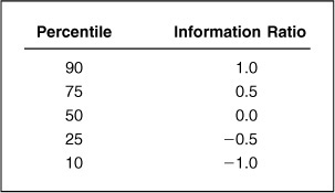
A top-quartile manager has an information ratio of one-half. That’s a good number to remember. Ex ante, investment managers should aspire to top-quartile status. Our analysis of a start-up investment manager’s information ratio, which we estimated at 0.64, provided a reasonable ballpark estimate, consistent with Table 5.1.
Table 5.1 displays a symmetric distribution of information ratios, centered on zero. This is consistent with our fundamental understanding of active management as a zero-sum game.
Table 5.1 also implies that if IR = 0.5 is good, then IR = 1.0 is exceptional. We will further define IR = 0.75 as very good and use that simple classification scheme throughout the book. Later in this chapter, we will provide more details on empirical observations of information ratios, as well as on active returns and active risk.
We will now define the information ratio in a more formal manner. Given an alpha for each stock, any (random) portfolio P will have a portfolio alpha αP and a portfolio residual risk ωP The information ratio for portfolio P is
Our personal “information ratio” is the maximum information ratio that we can attain over all possible portfolios:
So we measure our information ratio based on portfolios optimized to our alphas.
The notation IR hides the fact that the information ratio depends on the alphas. Indeed, one of the uses of the information ratio concept is to scale the alphas so that a reasonable value of IR is obtained through Eq. (5.6).
Our definition of the information ratio says that a manager who can get an expected residual return of 2 percent with 4 percent residual risk can also get an expected residual return of 3 percent with 6 percent residual risk. The ratio of risk to return stays constant and equal to the information ratio even as the level of risk changes. A small example will indicate that this is indeed the case.
We consider four stocks, cash, and a benchmark portfolio that is 25 percent in each of the stocks. Table 5.2 summarizes the situation. The alphas for both the benchmark portfolio (the weighted sum of the stock alphas) and cash are, of course, equal to zero. This is no accident.
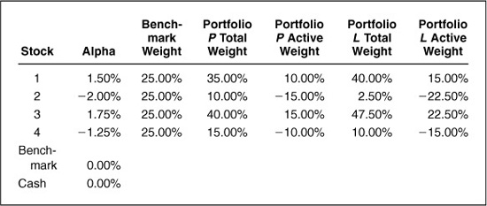
The last four columns describe two possible portfolios, P and L. For each portfolio, we have shown the portfolio’s total and active holdings. The active holdings are simply the portfolio holdings less the benchmark holdings. In portfolio P, we have positive active positions for the two stocks with positive alphas, and negative active positions for the stocks with negative alphas. Since the alpha for the benchmark is zero, we can calculate the alpha for the portfolio using only the active holdings.2 The alpha for portfolio P is
αp = >(1.50%) · (0.10) + (−2.00%) · (−0.15) + (1.75%) · (0.15) + (−1.25%) · (−0.10) = 0.84
The risk of this active position is 2.04 percent.3
Notice that portfolio L is just a more aggressive version of portfolio P. This isn’t clear when we look at the holdings in portfolio L, but it is obvious when we look at the active holdings. The active holdings of portfolio L are 50 percent greater than the active holdings of portfolio P. For stock 1, our active position goes from +10 percent to +15 percent. For stock 2, our active position goes from −15 percent to −22.5 percent. In both cases, the active position increases by 50 percent. This means that the alpha for portfolio L must be 50 percent larger as well, and that the active risk is also 50 percent higher.4 If both the portfolio alpha and the residual risk increase by 50 percent, the ratio of the two will remain the same.
The information ratio is independent of the manager’s level of aggressiveness.
We will consistently assume that the information ratio is independent of the level of risk. This relationship eventually breaks down in real-world applications, because of constraints. So in Table 5.2, if there is a constraint on short selling, we have little additional room to bet against stock 2 beyond portfolio L. Chapter 15, “Long/Short Investing,” expands on this idea, estimating a cost for the no short selling constraint based on the effective reduction in information ratio.
Although the information ratio is independent of the level of aggressiveness, it does depend on the time horizon. In order to avoid confusion, we standardize by using a 1-year horizon. The reason is that expected returns and variances both tend to grow with the length of the horizon. Therefore risk, standard deviation, will grow as the square root of the horizon, and the ratio of expected return (growing with time) to risk (growing as the square root of time) will increase with the square root of time. That means that the quarterly information ratio is half as large as the annual information ratio. The monthly information ratio would be  the size of the annual information ratio.
The choices available to the active manager are easier to see if we look at the alpha versus residual risk trade-offs. The residual frontier will describe the opportunities available to the active manager. The ex ante information ratio determines the manager’s residual frontier.
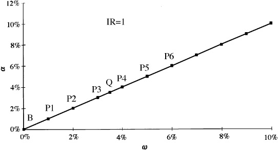
Figure 5.1 The residual frontier.
In Fig. 5.1 we have the residual frontier for an exceptional manager with an information ratio of 1. This residual frontier plots expected residual return αP, against residual risk ωP. The residual frontier is a straight line through the origin. Notice that portfolio Q is on the frontier. Portfolio Q is a solution to Eq. (5.6); i.e., IR = IRQ. Portfolio Q is not alone on the residual frontier. The portfolios P1, P2, uptoP6 are also on the residual frontier. The manager can attain any expected residual return and residual risk combination below the frontier line. Portfolios P1 through P6 have (respectively) 1 percent to 6 percent expected residual return and residual risk.
The origin, designated B, represents the benchmark portfolio. The benchmark, by definition, has no residual return, and thus both αB and ωB are equal to zero. Likewise, the risk-free asset will reside at the origin, since the risk-free asset also has a zero residual return.
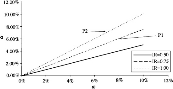
In Fig. 5.2 we show the residual frontiers of three different managers. The good manager has an information ratio of 0.5, the very good manager has an information ratio of 0.75, and the exceptional manager has an information ratio of 1.00.
We can see from Fig. 5.2 that the information ratio indicates opportunity. The manager with an information ratio of 0.75 has choices—portfolio P1, for example—that are not available to the manager with an information ratio of 0.5. Similarly, the exceptional manager has opportunities—at point P2, for example—that are not available to the very good manager. This doesn’t mean that the very good manager cannot hold the stocks in portfolio P2. It does mean that this very good manager’s information will not lead him or her to that portfolio; it will, instead, lead this manager to a portfolio like P1 that is on his or her residual frontier.
Effectively, the information ratio defines a “budget constraint” for the active manager, as depicted graphically by the residual frontier:
At best (i.e., along the frontier), the manager can increase the expected residual return only through a corresponding increase in residual risk.
The appendix contains a wealth of technical detail about information ratios. We now turn our attention from the manager’s opportunities to her or his objectives.
The objective of active management (derived in Chap. 4) is to maximize the value added from residual return, where value added is measured as5
This objective awards a credit for the expected residual return and a debit for residual risk. The parameter λR measures the aversion to residual risk; it transforms residual variance into a loss in alpha. In Fig. 5.3 we show the loss in alpha for different levels of residual risk. The three curves show high (λR = 0.15), moderate (λR = 0.10), and low (λR = 0.05) levels of residual risk aversion. In each case, the loss increases with the square of the residual risk ωP. For a residual risk of ωP = 5%, the losses are 3.75 percent, 2.5 percent, and 1.25 percent, respectively, for the high, moderate, and low levels of residual risk aversion.
The lines of equal value added, plotted as functions of expected residual return αP and residual risk ωP are parabolas. In Fig. 5.4 we have plotted three such parabolas for value added of 2.5 percent, 1.4 percent, and 0.625 percent. These curves are of the form  , αP = 1.4 + λR · ω2P, and αP = 0.625 + λR · ω2P. The figure shows the situation when we have a moderate level of residual risk aversion λR = 0.10. The three parabolas are parallel and increasing to the right. Every point along the top curve has a value added of 2.5 percent. The point {α = 2.5 percent, ω = 0 percent} and the point {α = 4.1 percent, ω = 4 percent} are on this curve. At the first point, with zero residual risk and an alpha of 2.5 percent, we have a value added of 2.5 percent. At the second point, the value added is still 2.5 percent, although we have risk. Thus, with ω = 4 percent and α = 4.1 percent, we have VA = 2.5 = 4.1 — (0.1) · 42.
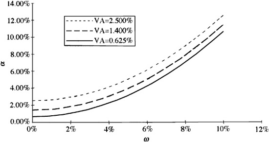
Figure 5.4 Constant value added lines.
We sometimes refer to the value added as the certainty equivalent return. Given a risk aversion λR, the investor will equate return αp and risk ωP with a certain return  to a (residual) riskfree investment.
It is a basic tenet of economics that people prefer more to less. Our choices are limited by our opportunities. We have to choose in a manner that is consistent with our opportunities. The information ratio describes the opportunities open to the active manager. The active manager should explore those opportunities and choose the portfolio that maximizes value added.
Figure 5.5 shows the situation. The residual frontier corresponds to an information ratio of 0.75 and a residual risk aversion of λR = 0.1. Preferences are shown by the three preference curves, with risk-adjusted returns of 0.625 percent, 1.40 percent, and 2.5 percent, respectively.
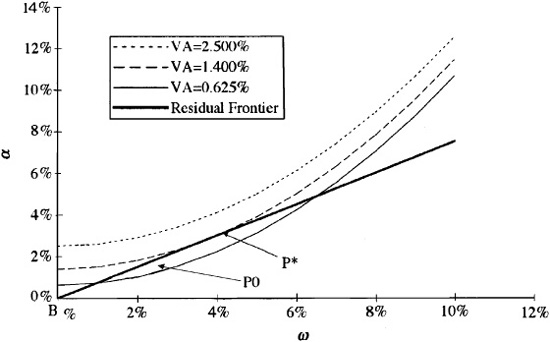
We would like to have a risk-adjusted return of 2.5 percent. We can’t do that well. The VA = 2.5 percent curve lies above the residual frontier. Life is a bit like that. We can achieve a risk-adjusted return of 0.625 percent. A value added of 0.625 percent is consistent with our opportunities; however, we can do better. Portfolio P0 is in the opportunity set and is better than 0.625 percent.
The 1.40 percent curve is just right. The 1.4 percent value added curve is tangent to the residual frontier at portfolio P*. We can’t do any better, since every higher-value added line is outside the opportunity set. Therefore, portfolio P* is our optimal choice.
The manager’s information ratio and residual risk aversion determine a simple rule that links those concepts with the manager’s optimal level of residual risk or aggressiveness. We can discover the rule through a more formal examination of the graphical analysis carried out in the last section.
The manager will want to choose a portfolio6 on the residual frontier. The only question is the manager’s level of aggressiveness. Using the “budget constraint” [Eq. (5.7)] in the manager’s objective, Eq. (5.8), we find
Now we have completely parameterized the problem in terms of risk. As we increase risk, we increase expected return and we increase the penalty for risk. Figure 5.6 shows the situation, representing the median case with IR = 0.75 and λR = 0.10.
The optimal level of residual risk, ω*, which maximizes VA [ωP]is
This is certainly a sensible result. Our desired level of residual risk will increase with our opportunities and decrease with our residual risk aversion. Doubling the information ratio will double the opti>mal risk level. Doubling the risk aversion will halve the optimal risk level.
Table 5.3 shows how the residual risk will vary for reasonable values of the information ratio and residual risk aversion. The information ratio has three possible levels: 0.50 (good), 0.75 (very good), and 1.0 (exceptional). The residual risk aversion also has three possible levels: 0.05 (aggressive), 0.1 (moderate), and 0.15 (restrained).

The highest level of aggressiveness is 10 percent, corresponding to the low residual risk aversion (λR = 0.05) and the high information ratio (IR = 1.00). At the other corner, with fewer opportunities (IR = 0.50) and more restraint (λR = 0.15), we have an annual residual risk of 1.67 percent. Table 5.3 is quite useful; it allows a manager to link two alien concepts, the information ratio and residual risk aversion, to the more specific notion of the amount of residual risk in the portfolio. We see that the greater our opportunities, the higher the level of aggressiveness, and the lower the residual risk aversion, the greater the level of aggressiveness. The table also helps us calibrate our sensibilities as to reasonable levels of IR and λR. Equation (5.10) will tell us if any suggested levels of IR and λR are reasonable.
It is possible to turn the question around and use Eq. (5.10) to determine a reasonable level of residual risk aversion. Recall the information ratio analysis earlier in the chapter. We determined that the manager wanted 5.5 percent residual risk and had an information ratio of 0.64. We can rearrange Eq. (5.10) and extract an implied level of residual risk aversion:
For our example, we have 0.64/(2 · 5.5) = 0.058. The manager is aggressive, with risk aversion at the lower end of the spectrum.
We have located the optimal portfolio P* at the point where the residual frontier is tangent to a preference line, and we have found a simple expression for the level of residual risk for the optimal portfolio. In this section, we will go one step further and determine the risk-adjusted residual return of the optimal portfolio P*.
If we substitute the optimal level of residual risk [Eq. (5.10)] into Eq. (5.9), we find the relationship between the value added as measured by utility and the manager’s opportunity as measured by the information ratio IR:
This says that the ability of the manager to add value increases as the square of the information ratio and decreases as the manager becomes more risk-averse. So a manager’s information ratio determines his or her potential to add value.
Equation (5.12) states a critical result. Imagine we are risk-verse investors, with high λR. According to Equation (5.12), given our λR, we will maximize our value added by choosing the investment strategy (or manager) with the highest IR. But a very risk-tolerant investor will make exactly the same calculation. In fact, every investor seeks the strategy or manager with the highest information ratio. Different investors will differ only in how aggressively they implement the strategy.
Table 5.4 shows the value added for the same three choices of information ratio and residual risk aversion used in Table 5.3. In our best case, the value added is 5.00 percent per year. That is probably more than one could expect. In the worst case, the value added is 42 basis points per year. A good manager (IR = 0.50) with a conservative implementation (λR = 0.15, so ω* = 1.66) will probably not add enough value to justify an active fee.
In our initial analysis of a manager’s information ratio, we found IR = 0.64 and λR = 0.058, and so the value added is 1.77 percent per year.

How do our residual risk/return choices look in the total risk/total return picture? The portfolios we will select (in the absence of any benchmark timing) will lie along the β = 1 frontier. This is the set of all portfolios with beta equal to 1 that are efficient; i.e., they have the minimum risk for a specified level of expected return. They are not necessarily fully invested. We develop this concept more fully in the technical appendix.
Figure 5.7 compares different efficient frontiers. The efficient frontier is the straight line through F and Q. The efficient frontier for fully invested portfolios starts at C and runs through Q. The efficient frontier for portfolios with beta equal to 1 starts at the benchmark, B, and runs through P.
The benchmark is the minimum-risk portfolio with β = 1, since it has zero residual risk. All other β = 1 portfolios have the same systematic risk, but more residual risk.
A glance at Fig. 5.7 may make us rethink our value added objective. There are obviously portfolios that dominate the β = 1 frontier. However, these portfolios have a large amount of active risk, and therefore expose the manager to the business risk of poor relative performance.
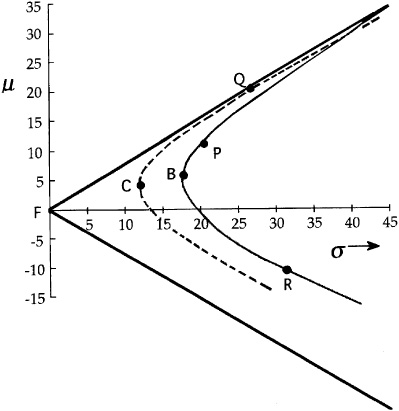
These two frontiers cross at the point along the fully invested frontier with β = 1. This crossing point will typically involve high levels of residual risk.
If we require our portfolios to satisfy a no active cash condition, then we have the situation shown in Fig. 5.8. The β = 1 no active cash frontier is the parabola centered on the benchmark portfolio B and passing through the portfolio Y. This efficient frontier combines the restriction to full investment (assuming that the benchmark is fully invested) with the β = 1 restriction. The opportunities without the no active cash restriction dominate those with the restriction. A constraint reduces our opportunities.
We have decided to manage relative to a benchmark and (at least until Chap. 19) to forgo benchmark timing. We have a need for alphas. We will discuss this topic at great length in the remainder of the book. However, we would like to show at this early stage that it isn’t very hard to produce a rudimentary set of alphas with a small amount of work. One way to get these alphas is to start with expected returns and then go through the complicated procedure described in Chap. 4. An alternative is to skip the intermediate steps and forecast the alphas directly. In fact, one of the goals of developing the active management machinery is to avoid having to forecast several quantities (like the expected return to the benchmark) which probably will not ultimately influence our portfolio. Here, then, is a reasonable example of what we mean, converting a simple ranking of stocks into alpha forecasts. To start, sort the assets into five bins: strong buy, buy, hold, sell, and strong sell. Assign them respective alphas of 2.00 percent, 1.00 percent, 0.00 percent, −1.00 percent, and −2.00 percent. Then find the benchmark average alpha. If it is zero, we are finished. If it isn’t zero (and there is no guarantee that it will be), modify the alphas by subtracting the benchmark average times the stock’s beta from each original alpha.
These alphas will be benchmark-neutral. In the absence of constraints, they should lead7 the manager to hold a portfolio with a beta of 1.00. One can imagine more and more elaborate variations on this theme. For example, we could classify stocks into economic sectors and then sort them into strong buy, buy, hold, sell, and strong sell bins.
This example illustrates two points. First, we need not forecast alphas with laserlike precision. We will see in Chap. 6, “The Fundamental Law of Active Management,” that the accuracy of a successful forecaster of alphas is apt to be fairly low. Any procedure that keeps the process simple and moving in the correct direction will probably compensate for losses in accuracy in the second and third decimal places. Second, although it may be difficult to forecast alphas correctly, it is not difficult to forecast alphas directly.
This section looks in more detail at the empirical results concerning active manager information ratios and risk.
Earlier, we described the “generic” distribution of before-fee information ratios. This generic distribution seems to apply across many different asset classes, stocks to bonds to international. Here we will present some of the empirical observations underlying the generic result.
These results were produced and partly described in Kahn and Rudd (1995, 1997). They arise from analysis of active U.S. domestic equity and bond mutual funds and institutional portfolios. These empirical studies utilized style analysis, which we describe in Chap. 17, “Performance Analysis.” Suffice it to say that this analysis allows us to estimate several empirical distributions of interest here. Table 5.5 briefly describes the data underlying the results that follow. The time periods involved are admittedly short, in part because style analysis requires an extensive in-sample period to determine a custom benchmark for each fund. The good news is that these are out-of-sample results. The bad news is that they do not cover an extensive time period.
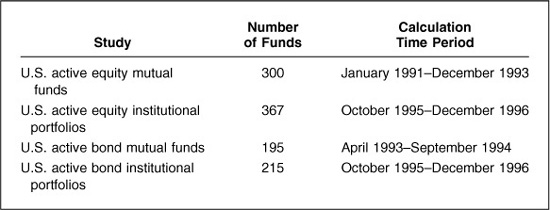
TABLE 5.6
Information Ratios, U.S. Active Equity Investments
The short time period will not bias the median estimates, but the large sample errors associated with the short time period will broaden the distributions.8 The problem is more severe for institutional portfolios, where we have only quarterly return data, and hence a smaller number of observations.
Tables 5.6 and 5.7 display empirical distributions of information ratios for equity and bond investors, respectively. These tables generally support the generic distribution of Table 5.1, especially considering that all empirical results will depend on time period, analysis methodology, etc.
TABLE 5.7
Information Ratios, U.S. Active Bond Investments
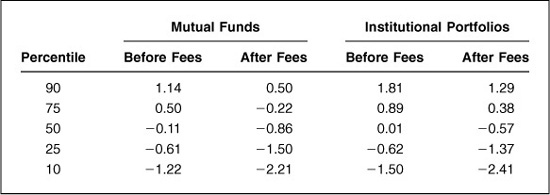
For equity investors, the empirical data show that top-quartile investors achieve information ratios of 0.63 to 0.78 before fees and 0.58 to 0.48 after fees. Given the standard errors for these results of roughly 0.05, and the fact that estimation errors tend to broaden the distribution, these empirical results are roughly consistent with Table 5.1.
The before-fee data on bond managers look roughly similar to the equity results, with top-quartile information ratios ranging from 0.50 to 0.89. The after-fee results differ strikingly from the equity manager results. For more on this phenomenon, see Kahn (1998).
Overall, given these empirical results, Table 5.1 appears to be a very good ex ante distribution of information ratios, before fees.
We can also look at distributions of active risk. Tables 5.8 and 5.9 show the distributions. Active managers should find this risk information useful: It helps define manager aggressiveness relative to the broad universe of active managers.
For equity managers, median active risk falls between 4 and 5 percent. Mutual fund risk resembles institutional portfolio risk, except at the low-risk end of the spectrum, where institutional managers offer lower-risk products.
For active domestic bond managers, the risk distributions vary between mutual funds and institutional portfolios, although both are well below the active equity risk distribution. Median active risk is 1.33 percent for bond mutual funds and only 0.61 percent for institutional bond portfolios.
TABLE 5.8
Annual Active Risk, U.S. Active Equity Investments
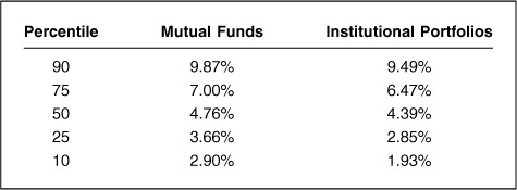
TABLE 5.9
Annual Active Risk, U.S. Active Bond Investments
We have built a simple framework for the management of residual risk and return. There are two key constructs in this framework:
■ The information ratio as a measure of our opportunities
■ The residual risk aversion as a measure of our willingness to exploit those opportunities
These two constructs determine our desired level of residual risk [Eq. (5.10)] and our ability to add value [Equation (5.12)]. In the next chapter, we will push this analysis further to uncover some of the structure that leads to the information ratio.
1. What is the information ratio of a passive manager?
2. What is the information ratio required to add a risk-adjusted return of 2.5 percent with a moderate risk aversion level of 0.10? What level of active risk would that require?
3. Starting with the universe of MMI stocks, we make the assumptions
Q = MMI portfolio
fQ = 6%
B = capitalization-weighted MMI portfolio
We calculate (as of January 1995) that

where portfolio C is the minimum-variance (fully invested) portfolio. For each portfolio (Q, B, and C), calculate f, α, ω, SR, and IR.
4. You have a residual risk aversion of λR = 0.12 and an information ratio of IR = 0.60. What is your optimal level of residual risk? What is your optimal value added?
5. Oops. In fact, your information ratio is really only IR = 0.30. How much value added have you lost by setting your residual risk level according to Problem 4 instead of at its correct optimal level?
6. You are an active manager with an information ratio of IR = 0.50 (top quartile) and a target level of residual risk of 4 percent. What residual risk aversion should lead to that level of risk?
Ambachtsheer, Keith. “Where are the Customer’s Alphas?” Journal of Portfolio Management, vol. 4, no. 1, Fall 1977, pp. 52-56.
Goodwin, Thomas H. “The Information Ratio.” Financial Analysts Journal, vol. 54, no. 4, July/August 1998, pp. 34-43.
Kahn, Ronald N. “Bond Managers Need to Take More Risk.” Journal of Portfolio Management, vol. 24, no. 3, Spring 1998, pp. 70-76.
Kahn, Ronald N., and Andrew Rudd. “Does Historical Performance Predict Future Performance?” Financial Analysts Journal, vol. 51, no. 6, November/December 1995, pp. 43-52.
——. “The Persistence of Equity Style Performance: Evidence from Mutual Fund Data.” In The Handbook of Equity Style Management, 2d ed., edited by Daniel T. Coggin, Frank J. Fabozzi, and Robert Arnott (New Hope, PA: Frank J. Fabozzi Associates), 1997, pp. 257-267.
——. “The Persistence of Fixed Income Style Performance: Evidence from Mutual Fund Data.” In Managing Fixed Income Portfolios, edited by Frank J. Fabozzi (New Hope, PA: Frank J. Fabozzi Associates), 1997, pp. 299-307.
Roll, Richard. “A Mean/Variance Analysis of Tracking Error.” Journal of Portfolio Management, vol. 18, no. 4, Summer 1992, pp. 13-23.
Rosenberg, Barr. “Security Appraisal and Unsystematic Risk in Institutional Investment.” Proceedings of the Seminar on the Analysis of Security Prices (Chicago: University of Chicago Press), November 1976, pp. 171-237.
Rudd, Andrew, and Henry K. Clasing, Jr. Modern Portfolio Theory, 2d ed.. (Orinda, Calif.: Andrew Rudd, 1988).
Sharpe, William F. “The Sharpe Ratio.” Journal of Portfolio Management, vol. 21, no. 1, Fall 1994, pp. 49-59.
Treynor, Jack, and Fischer Black. “How to Use Security Analysis to Improve Portfolio Selection.” Journal of Business, vol. 46, no. 1, January 1973, pp. 66-86.
Our basic input is a vector of asset alphas: α = {α1, α2, αN}. The alpha for asset n is a forecast of asset n’s expected residual return, where we define residual relative to the benchmark portfolio. Since the alphas are forecasts of residual return, both the benchmark and the risk-free asset will have alphas of zero; i.e., αB = αF = 0.
The characteristic portfolio of the alphas (see the appendix to Chap. 2) will exploit the information as efficiently as possible. Call portfolio A the characteristic portfolio of the alphas:
Portfolio A has an alpha of 1,  , and it has minimum risk among all portfolios with that property. The variance of portfolio A is
In addition, we can define alpha in terms of Portfolio A:
For any portfolio P with ωP > 0, define IRP as
If ωP = 0, we set IRP = 0. We call IRP the information ratio of portfolio P. We define the information ratio IR as the largest possible value of IRP given alphas {αn}, i.e.,
In the technical appendix to Chap. 2, we identified portfolio Q as the fully invested portfolio with the maximum Sharpe ratio, the ratio of expected excess return per unit of risk. Portfolio Q maximizes fP/(σP over all portfolios P. In this appendix, we will establish a link between portfolio Q, portfolio A, and the information ratio.
Portfolio A has the following list of interesting properties.
1. Portfolio A has a zero beta;  . It therefore typically has long and short positions.
2. Portfolio A has the maximum information ratio:
3. Portfolio A has total and residual risk equal to 1 divided by IR:
4. Any portfolio P that can be written as
has IRP = IR.
5. Portfolio Q is a mixture of the benchmark and portfolio A:
where
and
Therefore IRQ = IR. The information ratio of portfolio Q equals that of portfolio A.
6. Total holdings in risky assets for Portfolio A are
7. Let θP be the residual return on any portfolio P. The information ratio of portfolio P is
8. The (maximum) information ratio is related to portfolio Q’s (maximum) Sharpe ratio:
9. We can represent alpha as
Equation (5A.15) is an important result. It directly relates alphas to marginal contributions to residual risk, with the information ratio as the constant of proportionality. Thus, active managers should always check the marginal contributions to residual risk within their portfolios. For example, if they have an information ratio of 0.5, then half the marginal contributions should equal their alphas. This is a very useful check, especially on portfolios constructed by hand (as opposed to using an optimizer).
10. The Sharpe ratio of the benchmark is related to the maximal information ratio and Sharpe ratio:
Proof We verify the properties directly.
For item 1, recall from the appendix to Chap. 2 that since hB is the characteristic portfolio of beta and hA is the characteristic portfolio of alpha, we have  . Thus αB = 0 implies βA = 0. It isn’t surprising that αB = 0. The characteristic portfolio for beta has minimum risk given β = 1. It has zero residual risk, and hence zero alpha. Portfolio A has minimum risk given α = 1. Since it bets on residual returns, we would expect it to have minimum systematic risk, i.e., β = 0.
For item 2, consider any portfolio L with holdings hL. For any βP and scalar K > 0, we can construct another portfolio P with holdings
The residual holdings of P and L are proportional. Thus  and
and  and IRL = IRP When looking for a portfolio with a maximum information ratio, we might as well restrict ourselves to portfolios with beta of 0 and alpha of 1. Portfolio A has minimum risk among all such portfolios; therefore A has the maximum information ratio.
We can verify item 3 using Eq. (5A.2) and (5A.6), and the fact that βA = 0.
We can verify item 4 using Eq. (5A.17), with L equal to A and K =αP > >0.
For item 5, write the expected excess returns as
and as
since Q is proportional to the characteristic portfolio of f. Equating Eqs. (5A.18) and (5A.19) and multiplying by V−1, leads to
Premultiplying by  , and recalling that σA = ωA, leads to
This verifies Eqs. (5A.9) through (5A.11), and item 4 tells us that IRQ = IR.
We can verify item 6 by using the fact that portfolio C is the characteristic portfolio of e, the vector of all ones. Hence we have 
To verify item 7, for any portfolio P, we can write
Since portfolio A has a beta of 0, we can write
where θP and θA are the residual returns on portfolios P and A. If we divide Eq. (5A.22) by the residual risk of portfolio P, ωP find
Notice that  , so the residual returns on portfolios A and Q are perfectly correlated, and thus Corr{θP, θA} = Corr{θP, θQ}.
For item 8, start with Eq. (5A.11) and divide both sides by αQ. Then use the facts that  , SR = fQ/σQ, and IR = 1/ωA.
We can prove the first part of item 9 by using Eq. (5A.3) and the fact that IR = 1/ωA. The marginal contribution to residual risk of asset n in portfolio Q is Cov{θQ, θn}/ωQ. However, the residual holdings of portfolio Q are αQ · hA, and the residual risk of portfolio Q is  . Thus,
  .
.
To prove item 10, recall that  and
and  . Then use
  , which is just
  and
and  . The last relationship follows since the benchmark is the characteristic portfolio of beta (see the appendix to Chap. 2).
Portfolio A is key to the problem of finding an optimal residual position. Consider the problem
The optimal solutions to Eqs. (5A.25) are given by
where βP is arbitrary.
The value added by the optimal solution is
and the residual volatility of the optimal solution is
Proof The first-order conditions for the problem in Eq. (5A.25) are
A solution is optimal if and only if hP solves Eq. (5A.29). Let  . This yields
Now substitute for alpha using Eq. (5A.3) and for  with
with  . The result is
Multiply Eq. (5A.31) by V-1, and divide by  . This yields Eq. (5A.26). Equation (5A.28) follows, since hA/ωA has residual volatility equal to 1. For Eq. (5A.27), substitute the optimal solution, Eq. (5A.26), in the objective and gather terms.
Notice that hP will have beta equal to βP, so we are consistent. It should be obvious that beta is irrelevant for the problem in Eq. (5A.26). The alphas are benchmark-neutral, so the alpha part of the objective in Eq. (5A.26) does not change as the portfolio’s beta changes. Also, the residual risk is independent of the portfolio beta, and so ωP will be independent of βP as well.
Our analysis to this point will let us specify the set of efficient portfolios that are constrained to have beta equal to 1, a fixed level of expected return, and minimal risk. These are interesting portfolios for institutional active managers. (There is a reason that we have relegated benchmark timing to the end of the book.) Since we will require beta equal to 1, the risk and expected return will be given by
and
The benchmark is the minimum-variance portfolio with beta equal to 1. The benchmark is the hinge in the β = 1 frontier in the same way that portfolio C is the hinge for the frontier of fully invested portfolios. To be on the β= 1 frontier, a portfolio must have a beta equal to 1 and a minimal amount of residual risk per unit of alpha. These will be portfolios on the alpha/residual risk efficient frontier, with ratios of alpha to residual risk equal to the information ratio. The residual variance is given by
When we combine these last three equations, we have the equation for the β= 1 frontier:
Portfolio A is the minimum-variance portfolio that has a unit exposure to alpha. However, it may turn out that portfolio A has a large positive or negative cash exposure. In active management, we often wish to move away from our benchmark and toward an efficient implementation of our alphas, while assuming no active cash position or active beta. But from item 6 of Proposition 1, we see that eA = 0 if and only if αC = 0. Here we will introduce a new portfolio, portfolio Y, and discuss its properties. In the next section we will show that portfolio Y is the solution to the problem of optimizing our alphas subject to active cash and beta constraints.
To begin, define the residual holdings of portfolio C as
Portfolio Y is a combination of portfolio A and portfolio CR:
Portfolio Y has the following properties:
1. Portfolio Y has a zero beta; βY = 0.
2. Portfolio Y has total and residual variance
3. Portfolio Y has an alpha given by
4. Portfolio Y has a zero cash position: eY = 0. Note that Y is an active position. Property 4 guarantees that its long risky holdings exactly match its short risky holdings, and hence its cash position must be zero.
5. Portfolio Y has an information ratio
Proof Item 1 follows because hY is a linear combination of two portfolios, each with zero beta.
To show item 2, calculate the variance of hY using Eq. (5A.37). To calculate the covariance of hA and hCR, note that  , and that the covariance between hCR and hA is the same as the covariance between hC and hA since portfolio A is pure residual.
Item 3 follows by direct calculation starting with Eq. (5A.37).
To prove item 4, use  and
and  .
.
Item 5 is a direct result of items 2 and 3.
Portfolio Y is linked to the problem of finding an optimal residual position under the restrictions of no active beta and no active cash. The problem is
subject to  and
and  .
.
The optimal solution of Eq. (5A.41) is
Proof The constraints dictate that the optimal solution to the problem must be of the form hP = hB + hPR, where hPR is a residual position with no active cash, i.e.,  . We will associate the rather strange Lagrange multipliers
  and
and  with the beta and holdings constraints, respectively. The first-order conditions are the two constraints, plus
In Eq. (5A.43), we can write α as  as
as  , and
, and  as
as  . If we make those substitutions, multiply by V−1, and divide by
  , we find
The constraints on beta and total holdings along with  allow us to solve for Φ and ω. The solutions are
When we combine these results, we find  , the desired result.
Thus far in this technical appendix, we have described key portfolios involved in managing residual risk and return, and have discussed how these affect our understanding of the information ratio. At this point, we turn to two more mundane properties of the information ratio: how it scales with investment time period and with the scale of the alphas.
Consider a time period of length T years. If the residual return in any time interval is independent of the residual returns in other time intervals, and the residual returns have the same mean and standard deviation in all time intervals, then the ratio of the residual return over the period [0,T] to the residual risk over the period [0,T] will grow with the square root of T.
Proof Divide the period [0,T] into K intervals of length Δt = T/K. Let k = 1,2,..., K index the intervals; interval k runs from time  to k · Δt. Let θ(k) be the residual return in interval k, and let
  be the residual return over [0,T]. The expected value of θ(k) is the same for all k—say, α = E{θ(k)}—and so
The θ(k) have a constant variance, Var{θ(k)} = ω2. Since the θ(k)are independent, we have
and
Therefore,
which is the promised result. Note that the annual information ratio is 
The information ratio is linear in the input alphas.
Proof Rescale α by a factor π in Eq. (5A.6). The resulting information ratio is π · IR.
We find this obvious result quite useful. One difficulty that arises in practice is the use of alphas that are so optimistic that they overwhelm any reasonable constraints on risk. The alphas usually need to be scaled down. Given a set of alphas, one could calculate (there are programs that do this)  . Suppose we find IR0 = 2.46. We know from our common-sense discussion in this chapter that numbers like 0.75 are more reasonable. If we multiply the alphas by π = 0.75/2.46, then the information ratio for the scaled alphas will be 0.75. We could put these scaled alphas into an optimization program with a reasonable level of active risk aversion (λ = 0.10) and expect plausible results.
1. Demonstrate that

2. Demonstrate that

Note that βc = (σC/σB)2. In the absence of benchmark timing, i.e., if fB = μB, the alpha of portfolio C is the key to determining the beta of portfolio Q.
For these exercises, assume that
Portfolio B = CAPMMI
Portfolio Q = MMI
fQ = 6 percent
Applications Exercises 1, 2, and 3 are closely related to Problem 3 at the end of the main body of this chapter. The difference is that here you need to supply all the numbers.
1. What are the expected excess returns and residual returns for portfolios B, Q, and C?
2. What are the total and residual risks for portfolios B, Q, and C?
3. What are the Sharpe ratios and information ratios for portfolios B, Q, and C?
4. Demonstrate Eq. (5A.16).