CHAPTER 18
Expected Returns and Risks from Direct Lending
Previous chapters discussed the different dimensions of corporate direct lending. This chapter and the next provide an institutional framework for assessing direct lending relative to other asset classes and determining the appropriate allocation to direct lending within an overall portfolio.
Somewhat surprisingly, the institutional approach to asset allocation has not changed much over the past 40 years. Prior to 1980, a centralized top–down approach to asset allocation did not exist. Instead institutional investors allocated assets to a few good balanced managers who made decisions as to how to allocate assets across different asset classes, which at that time were only a handful. Pensions, endowments, and foundations (collectively called fund sponsors) moved to a single‐allocator model in the 1980s because the balanced manager approach showed poor returns, charged high fees, and was not integrated with benefit obligations and spending rates. Consultants, who previously focused almost exclusively on manager selection, emerged to assist their institutional clients with asset allocation and asset‐liability management.
With control of asset allocation, fund sponsors and their consultants forecast long‐term return and risk for individual asset classes, define an efficient frontier of asset mixes that maximize return at different levels of risk, and select the asset mix from the efficient frontier that best fits the risk‐taking desired by the fund sponsor. The efficient‐frontier portfolio that best matches the level of risk desired by the fund sponsor is called the optimal portfolio, or more frequently the policy asset mix, and becomes part of the fund sponsor's investment policy statement (IPS). This process, known as an asset allocation study, is repeated every three to five years. Most asset allocation studies do not closely integrate liabilities into the selection of the policy asset mix except for corporate pension plans that have less tolerance for variability of required pension contributions. Corporate pension plans have sought to eliminate changes in their unfunded liabilities by matching the interest rate risk (duration) of their assets with that of their liabilities, which typically is in the 9–12‐year range.
The growth of corporate direct lending, or more broadly private debt, among institutional investors will partly depend upon its role within the context of asset allocation studies. A critical step will be for investment consultants, who have great influence over asset allocation decisions, to judge private debt as an investment that is sufficiently permanent, scalable, and unique in terms of possessing investment characteristics that are not otherwise incorporated in other mainstream asset classes already widely used in asset allocation studies. If this happens, private debt will become more widely used as a distinct asset class for asset allocation studies, and potentially a permanent fixture in policy asset mixes. That is now just starting to happen, as a small number of the largest US public pension systems are including private debt as a separate asset class within their policy asset mixes, at levels up to and sometimes exceeding 10% of total assets.
In cases where private debt is not modeled as a separate asset class, another factor that will affect the growth of its adoption by institutions is the choice of the broader asset class within which private debt is considered a subcategory. In some cases, private debt is included within a private equity, or private assets, program. Since most institutions view private equity as a return‐enhancing strategy, private debt, even though it may have superior risk‐adjusted returns than private equity, might be viewed as having a drag on performance. This can have a particularly dampening effect on the demand for private debt in cases where investment staffs receive performance‐based compensation. This can work in the opposite way when private debt is included within a broader fixed income allocation. In these cases, private debt can significantly enhance the yield and return profile of a public fixed income portfolio, even alongside high‐yield and other non‐investment‐grade debt exposure.
Chapter 7 presented the case for treating credit as a separate asset class. The purpose of this chapter is to provide the inputs necessary to integrate private debt into an asset‐allocation study.
EXPECTED RETURN
The following equation gives a simple and concise expression for determining expected return.
The two variables in brackets represent the strategic component of return because they incorporate long‐term asset class fundamentals, which returns will eventually mirror. The sum of current cash yield plus cash flow growth is often referred to as the Gordon model. Change in valuation measures the asset price changes that would come about, for example, if price‐to‐earnings ratios changed, if the yield curve shifted up or down, or if overall credit spreads shifted. Valuation changes are viewed as sources of short‐term volatility, with limited impact on long‐term returns. Therefore, this component is generally not included in the expected return estimate used in asset allocation studies. Finally, manager Alpha is the concept of managers creating idiosyncratic returns not attributable to the general market. Since manager Alpha is highly variable and ephemeral, it has generally been industry practice not to include manager Alpha into expected returns. The exception is for those asset classes that would otherwise not be considered for inclusion except for a significant, positive contribution from manager Alpha.
There are two asset classes for which manager Alpha is a significant contributor to expected returns, helping to drive allocations in a policy investment mix. The first is private equity. Allocators typically assume a return premium over public equity when developing their private equity expected returns, usually in the range of 2–3%. This premium might partly be attributable to a liquidity premium, in which case it is not alpha and would be reflected in an otherwise higher current cash yield compared to public stocks. The other source of the return premium is manager Alpha, which could come from opportunistically buying companies below their intrinsic value, or making improvements to the company's revenue growth and/or profitability in ways unique to the manager. For most asset classes, the uncertainty in forecasting for manager Alpha is high because these markets are generally efficient, and manager Alpha has not been found to be significant and persistent over an extended period. Private equity has been an exception to this, where excess returns have been significant and persistent. For example, data from state pension systems covering the period from 2002 to 2017 show that private equity portfolio returns in aggregate earned net returns equal to 10.7%, annualized, which exceeded public equity returns by 4.0%, justifying the inclusion of a return premium.
The second asset class where manager Alpha is integral to its expected return is hedge funds. A 2–3% manager Alpha is a typical range for modeling hedge fund expected returns. Also, investors don't generally think about cash yield and cash flow growth in the context of hedge funds. Instead a forecast of equity beta gives a percentage level of participation in overall stock market cash yield and cash flow growth. For example, if hedge funds are expected to have an equity beta equal to 0.20, and if expected stock cash yield plus cash flow growth equals 7%, then hedge funds will be expected to derive a 1.4% return (0.20 × 7%) from its exposure to stocks. The sum of 1.4% and the level of manager Alpha the allocator selects equals the expected return for hedge funds.
This backdrop should be useful for developing an expected return for corporate direct lending that is consistent with how expected returns are developed for other asset classes in an asset allocation study.
Fortunately, developing expected returns for corporate direct lending is straightforward with a likely lower estimation error than most other asset classes. Despite this, there are several nuances to consider.
Using the expected return equation above, a first try at forecasting cash yield might be either the current yield or yield‐to‐three‐year‐takeout for the Cliffwater Direct Lending Index (CDLI). The current yield on the CDLI is probably a better measure for calculating expected return because if net asset value (NAV) is at a premium or discount to principal value it assumes no amortization, while yield‐to‐three‐year‐takeout assumes a three‐year amortization window and, if used, would likely overstate long‐term expected returns. The current yield on the CDLI was 10.08% at December 31, 2017.
An adjustment to cash yield might be for expected changes in short‐term rates over the 10‐year forecasting period. Historically, short‐term rates have tracked expected inflation, but at December 31, 2017 the three‐month Treasury bill was yielding 1.38%, which was below the roughly 2.00% expected inflation over the subsequent 10 years. Depending upon when T‐bill yields rise, an upward adjustment to the 10.08% direct lending current yield might be warranted because loan benchmark rates are effectively tied to T‐bill yields. However, in the calculation of direct lending expected return below, no adjustment is made because any rate convergence to long‐term inflation is likely less certain that it has been in the past.
Using the CDLI current yield also assumes the risk premiums within the corporate direct lending market will remain consistent with the premiums measured at December 31, 2017. While the current premiums undoubtedly will move around over time, their current value will likely be an unbiased estimate of future premiums. Another approach could be to look at historical risk premiums or historical current yields for corporate direct lending and use those. The problem with this approach is that it ignores the starting point, to which expected returns can be very sensitive, even over 10‐year periods.
The second component of expected return, cash flow growth, is likely a negative number for direct lending and should be set to equal expected realized credit losses over the 10‐year forecasting period. The 1.05% annual rate in realized credit losses should be a good first approximation of future expected credit losses.
Finally, change in valuation is generally ignored for asset allocation studies. It is also less important for middle market direct lending where fundamentals and valuations are more stable and, unlike stock price‐earnings ratios, valuations are not subject to wide swings. Manager Alpha can also be ignored for expected return. CDLI returns and fundamentals reflect the weighted average efforts of the underlying managers and if manager Alpha exists it is already embedded into CDLI cash yield and cash flow growth.
Exhibit 18.1 provides a calculation for 10‐year return forecasts for corporate direct lending that would be suitable inputs into institutional asset allocation studies. Two prospective portfolios are modeled. The first column represents an unlevered direct lending portfolio and the second column represents a modestly levered portfolio.
EXHIBIT 18.1 Calculation of expected return for corporate direct lending.
| Unlevered Portfolio (%) | Levered Portfolio (%) | ||
| Assumptions | |||
| 1 | Gross yield on direct loans | 9.50 | 9.50 |
| 2 | Credit loss rate | −1.05 | −1.05 |
| 3 | Leverage | NA | 0.85x |
| 4 | Management fee (on net assets) | 1.25 | 1.25 |
| 5 | Incentive fee | NA | 10 |
| 6 | Preferred return | NA | 7 |
| 7 | Admin expenses (on net assets) | 0.25 | 0.25 |
| 8 | Cost of financing | NA | 4.50 |
| Expected Return Calculation | |||
| 9 | Unlevered portfolio cash yield | 9.50 | 9.50 |
| 10 | + Gross yield from leverage | NA | 8.08 |
| 11 | − Interest cost of leverage | NA | −3.83 |
| 12 | = Gross levered portfolio cash yield | 9.50 | 13.75 |
| 13 | − Expected credit loss | −1.05 | −1.94 |
| 14 | = Net yield before fees | 8.45 | 11.81 |
| 15 | − Management fees | −1.25 | −1.25 |
| 16 | − Administrative expenses | −0.25 | −0.25 |
| 17 | = Net yield after management fees and admission expenses | 6.95 | 10.31 |
| 18 | − Incentive fees | NA | −1.03 |
| 19 | = Expected return on direct lending | 6.95 | 9.28 |
| Notes | |||
| 20 | Total management and incentive fees | 1.25 | 2.28 |
| 21 | Fees as % of net yield before fees | 15 | 19 |
The assumptions in lines 1–8 are intended to mirror the typical investment characteristics and terms for a diversified direct lending portfolio. However, actual direct lending portfolio specifications can vary significantly, and portfolio size can alter terms. Consequently, the calculations in Exhibit 18.1 should be viewed as representative for corporate direct lending at December 31, 2017.
Expected gross yield equals 9.50% (line 1) and is slightly below the 10.16% interest income reported in Exhibit 2.3 for the CDLI during 2017. The lower yield is intended to blend somewhat lower yields on private funds that allocate higher amounts to senior loans. The 9.50% gross yield is assumed to be the same for both unlevered and levered strategies. Credit losses (line 2) equal the historical average realized losses for the CDLI. Leverage at 0.85x (line 3) lies roughly between the 0.72x average leverage for business development companies (BDCs) and the 0.93x average used by levered private funds. Management fees at 1.25% of net assets (line 4) is the most likely rate found for levered and unlevered funds charging on net assets rather than gross assets. The 10% incentive fee (line 5) is subject to a 7% preferred return (line 6), but it does not impact the expected return because the difference between the 10.31% net yield after management fees and administrative expenses in line 14 and the 7% preferred return exceeds the 1.03% incentive fee calculation (line 18). Administrative expenses (line 6) are assumed to equal 0.25% but they can vary in practice. Administrative expenses are generally lower for private funds and higher for registered vehicles like BDCs. Like management fees, administrative fees can sometimes be charged on gross assets. The 4.50% cost of financing the 0.85x leverage (line 8) approximately equals the annualized weighted average interest cost for obtaining leverage among BDCs during the fourth quarter of 2017.
With changing short‐term rates, it can be helpful to measure both direct loan yields and the cost of financing as a spread to three‐month Libor, a common benchmark rate for floating‐rate loans and estimating interest costs. Three‐month Libor averaged 1.50% during the fourth quarter of 2017, the period upon which the 9.50% gross direct loan yield and 4.50% financing cost are based. The net spread to Libor for direct loan yields and financing costs is therefore 8.00% and 3.00%, respectively. Should interest rates continue to rise, direct loan yields and financing costs will rise, increasing expected returns for both unlevered and levered direct loan portfolios.
The expected return calculation starts in line 9 with a 9.50% current yield for both unlevered and levered portfolios. The expected return on the unlevered portfolio is straightforward. Deductions for credit losses (line 13), management fees (line 15), and administrative expenses (line 16) leave a net yield and expected return equal to 6.95%. Manager fees (line 20) as a percent of net yield before fees (line 14) equals 15% (line 21).
The levered portfolio adds 8.08% (9.50% multiplied by 0.85) in leveraged yield (line 10) but deducts 3.83% (4.50% multiplied by 0.85) in financing costs, resulting in a 13.75% gross levered cash yield (line 12). Subtracting expected credit losses of 1.94% (1.05% multiplied by 1.85) gives a net yield before fees equal to 11.81%. Further, subtracting management fees and administrative expenses produces a 10.31% return (line 17) upon which incentive fees are based. The full incentive fee is equal to 1.03% (10% multiplied by 10.31%) and is deducted to arrive at an expected return equal to 9.28% for the levered direct lending portfolio (line 19). Total fees (line 20) as a percent of net yield before fees (line 14) equals 19% (line 21).
Looked at in isolation, most institutional investors should find corporate direct lending with a 6.95% unlevered or 9.28% levered expected return compelling when compared with recent total fund returns. A recent 17‐year performance study by Cliffwater LLC covering all state pension plans with fiscal years ended June 30, 2017, representing over $2.6 trillion in assets, found that pension assets produced a 5.69% compound annual return, far less than the 7–8% actuarial assumed returns. Since the 2000–2017 period covers two bear markets and two bull markets, the 5.69% return would seem very representative of what pensions might achieve looking ahead. By comparison, only 3 of the 66 state pensions in the study achieved returns above 6.95% over the 17 years.
In the same Cliffwater study, the average annual risk for individual state pension portfolios, measured by standard deviation, equaled 11.16% for the 17 years ending June 30, 2017. By comparison, the return standard deviation for the unlevered CDLI equaled 3.54% over the 13.25 years ending December 31, 2017. In Chapter 11, risk calculations for direct lending portfolios with various amounts of leverage were derived based on historical CDLI data and fee assumptions. Risk calculations ranged from a 3.18% standard deviation for an unlevered direct lending portfolio to 9.55% standard deviation for a direct lending portfolio at 2.0x leverage. Even at the high 2.0x leverage the direct lending portfolio risk is below the average total portfolio risk for state pensions. While the comparative time periods do not precisely overlap, it seems reasonable to conclude that the addition of corporate direct lending to large state pensions would be accretive, increasing pension returns and reducing risk. This outcome would be similar if applied to other institutional asset pools.
Asset allocation studies begin with a review of return assumptions for all available asset classes. Exhibit 18.2 provides a detailed matrix with expected returns, risks, and correlations for 23 traditional and alternative asset classes, most of which are considered in asset allocation studies. Expected returns are represented by the compound return in the first column and were created using the earlier equation and applying it to each asset class. Long‐term expected returns for major asset classes are generally similar across consultants and other allocators.
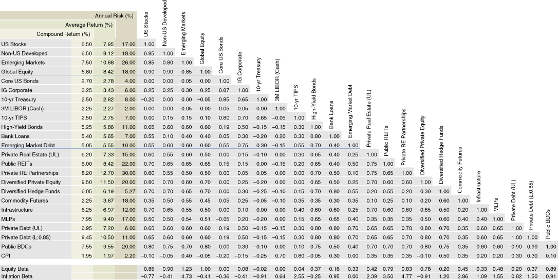
EXHIBIT 18.2 Expected return, risk, and correlations across asset classes.
EXPECTED RISKS
Expected risk is shown in the third column of Exhibit 18.2. The public asset classes rely upon historical measures alone. The private asset classes use historical data in combination with unsmoothing techniques and links to public asset classes to arrive at risk forecasts that are more economically based, rather than accounting based. For example, the risk forecast shown for unlevered private debt, which is based upon direct lending, equals 6.00%, which is higher than the 3.54% historical standard deviation in Exhibit 11.4 and the 4.59% unsmoothed risk calculation in Chapter 14. This second unsmoothing procedure links CDLI returns to publicly traded credit index returns, with lags, which provides a method for adjusting upward both correlations and standard deviations. Unlike expected returns, risk estimates for private asset classes can vary widely across consultants, who often use different techniques for forecasting risk.
Correlations are shown in the remaining columns in Exhibit 18.2. As with expected risk, correlation forecasts rely on historical measures for the liquid asset classes and unsmoothed mechanisms for the private asset classes.
Values for the Consumer Price Index (CPI) are added to the asset classes near the bottom of Exhibit 18.2, as many allocators want to gauge the sensitivity of their asset mix policies to changing inflation. This has received special interest recently with the concern over what will happen to asset values if inflation rises. The correlations of asset classes with CPI inform investors whether asset classes will react positively to rising inflation (positive correlation) or negatively to rising inflation (negative correlation). The last row shows the inflation beta, a measure of asset class return sensitivity to changes in CPI inflation. Note that unlevered direct lending has a forecast inflation beta equal to 0.82, meaning that if inflation unexpectedly increases 5.0% over some period, the return on direct lending will increase an additional 4.1% over the same period. This relationship is entirely consistent with the floating‐rate characteristic of direct loans. In contrast, conventional fixed income with a fixed rate has negative inflation betas. Core US bonds have an expected inflation beta equal to −0.36. This has also been consistent with rising rates over the past two years, where core bond portfolios with fixed interest rates have reported negative returns.
Also shown are equity betas for the asset classes in the second‐to‐last row. Direct lending is assumed to have a positive correlation with stocks and, unlevered, a 0.20 equity beta. This level of equity beta is also consistent with events during the 2008 global financial crisis. The CDLI fell 6.5% during calendar 2008, only 15% of the 42.2% drop in global stocks, measured by the MSCI All Country World Index.
Not so favorable is the high 0.80 correlation between direct lending and private equity. This level of correlation means that 64% (R‐square) of the variability in direct lending returns is explained by volatility in the underlying equity of the companies lent to. This also sounds reasonable given the Chapter 8 discussion of loans as a short put option on corporate assets. Volatility in the valuation of corporate assets is directly absorbed by corporate debt and equity with the split determined by the amount of leverage. In comparison to other asset classes, direct lending is attractive for being high‐cash‐yielding, low‐risk, and sensitive to positive interest rates and inflation. Its negatives are lack of liquidity and diversification potential. The lack of diversification also extends to publicly traded high‐yield bonds and bank loans, whose correlations with direct lending are also expected to be high because the underlying borrowers in all three asset classes are companies inextricably linked to the business cycle.