5
Architecture
From the intrinsic evidence of his creation, the Great Architect of the Universe now begins to appear as a pure mathematician.
Sir James Jeans, Mysterious Universe
Now that we have the mathematical and physical preliminaries under our belt, we can move on to the nuts and bolts of quantum computing. At the heart of a classical computer is the notion of a bit and at the heart of quantum computer is a generalization of the concept of a bit called a qubit, which shall be discussed in Section 5.1. In Section 5.2, classical (logical) gates, which manipulate bits, are presented from a new and different perspective. From this angle, it is easy to formulate the notion of quantum gates, which manipulate qubits. As mentioned in Chapters 3 and 4, the evolution of a quantum system is reversible, i.e., manipulations that can be done must also be able to be undone. This “undoing” translates into reversible gates, which are discussed in Section 5.3. We move on to quantum gates in Section 5.4.
Reader Tip. Discussion of the actual physical implementation of qubits and quantum gates is dealt with in Chapter 11. ![]()
5.1 BITS AND QUBITS
What is a bit?
Definition 5.1.1 A bit is a unit of information describing a two-dimensional classical system.
There are many examples of bits:
![]() A bit is electricity traveling through a circuit or not (or high and low).
A bit is electricity traveling through a circuit or not (or high and low).
![]() A bit is a way of denoting “true” or “false.”
A bit is a way of denoting “true” or “false.”
![]() A bit is a switch turned on or off.
A bit is a switch turned on or off.
![]()
All these examples are saying the same thing: a bit is a way of describing a system whose set of states is of size 2. We usually write these two possible states as 0 and 1, or F and T, etc.
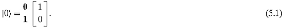
As we have become adept at matrices, let us use them as a way of representing a bit. We shall represent 0 – or, better, the state ![]() − as a 2-by-1 matrix with a 1 in the 0’s row and a 0 in the 1’s row:
− as a 2-by-1 matrix with a 1 in the 0’s row and a 0 in the 1’s row:
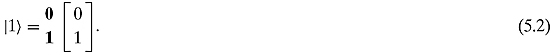
We shall represent a 1, or state ![]() , as
, as
Because these are two different representations (indeed orthogonal), we have an honest-to-goodness bit. We explore how to manipulate these bits in Section 5.2.
A bit can be either in state ![]() or in state
or in state ![]() , which was sufficient for the classical world. Either electricity is running through a circuit or it is not. Either a proposition is true or it is false. Either a switch is on or it is off. But either/or is not sufficient in the quantum world. In that world, there are situations where we are in one state and in the other simultaneously. In the realm of the quantum, there are systems where a switch is both on and off at the same time. One quantum system can be in state
, which was sufficient for the classical world. Either electricity is running through a circuit or it is not. Either a proposition is true or it is false. Either a switch is on or it is off. But either/or is not sufficient in the quantum world. In that world, there are situations where we are in one state and in the other simultaneously. In the realm of the quantum, there are systems where a switch is both on and off at the same time. One quantum system can be in state ![]() and in state
and in state ![]() simultaneously. Hence we are led to the definition of a qubit:
simultaneously. Hence we are led to the definition of a qubit:
Definition 5.1.2 A quantum bit or a qubit is a unit of information describing a two-dimensional quantum system.
We shall represent a qubit as a 2-by-1 matrix with complex numbers

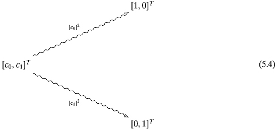
where |c0|2 + |c1|2 = 1. Notice that a classical bit is a special type of qubit. |c0|2 is to be interpreted as the probability that after measuring the qubit, it will be found in state ![]() . |c1|2 is to be interpreted as the probability that after measuring the qubit it will be found in state
. |c1|2 is to be interpreted as the probability that after measuring the qubit it will be found in state ![]() . Whenever we measure a qubit, it automatically becomes a bit. So we shall never “see” a general qubit. Nevertheless, they do exist and are the main characters in our tale. We might visualize this “collapsing” of a qubit to a bit as
. Whenever we measure a qubit, it automatically becomes a bit. So we shall never “see” a general qubit. Nevertheless, they do exist and are the main characters in our tale. We might visualize this “collapsing” of a qubit to a bit as
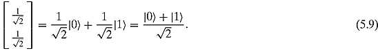
It is easy to see that the bits ![]() and
and ![]() are the canonical basis of
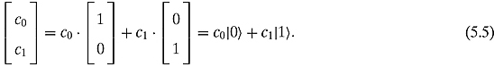
are the canonical basis of ![]() . Thus, any qubit can be written as
. Thus, any qubit can be written as
Exercise 5.1.1 Write ![]() as a sum of
as a sum of ![]() and
and ![]() .
.
![]()
Following the normalization procedures that we learned in Chapter 4 on page 109, any nonzero element of ![]() can be converted into a qubit.
can be converted into a qubit.
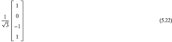
Example 5.1.1 The vector
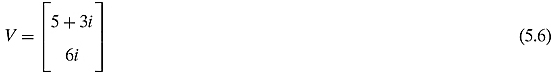
has norm

So V describes the same physical state as the qubit

After measuring the qubit ![]() , the probability of it being found in state
, the probability of it being found in state ![]() is
is ![]() and the probability of it being found in state
and the probability of it being found in state ![]() is
is ![]() .
.
![]()
Exercise 5.1.2 Normalize ![]()
![]()
Let us look at several ways of denoting different qubits. ![]() can be written as
can be written as
Similarly, ![]() can be written as
can be written as

It is important to realize that
![]()
These are both ways of denoting ![]() . In contrast,
. In contrast,
![]()
The left state is the vector ![]() and the right state is the vector
and the right state is the vector ![]() . However, the two states are related:
. However, the two states are related:
![]()
How are qubits to be implemented? In Chapter 11, several different methods are explored. We simply state some examples of implementations for the time being:
![]() An electron might be in one of two different orbits around the nucleus of an atom (ground state and excited state).
An electron might be in one of two different orbits around the nucleus of an atom (ground state and excited state).
![]() A photon might be in one of two polarized states.
A photon might be in one of two polarized states.
![]() A subatomic particle might have one of two spin directions.
A subatomic particle might have one of two spin directions.
There will be enough quantum indeterminacy and quantum superposition effects within all these systems to represent a qubit.
Computers with only one bit of storage are not very interesting. Similarly, we will need quantum devices with more than one qubit. Consider a byte, or eight bits. A typical byte might be
![]()
If we were to follow the preceding method of describing bits, we would represent the bits as follows:
We learned previously that in order to combine quantum systems, one should use the tensor product; hence, we can describe the byte in Equation (5.14) as
![]()
As a qubit, this is an element of
![]()
This vector space may be denoted as ![]() . This is a complex vector space of dimension 28 = 256. Because there is essentially only one complex vector space of this dimension, this vector space is isomorphic to
. This is a complex vector space of dimension 28 = 256. Because there is essentially only one complex vector space of this dimension, this vector space is isomorphic to ![]() .
.
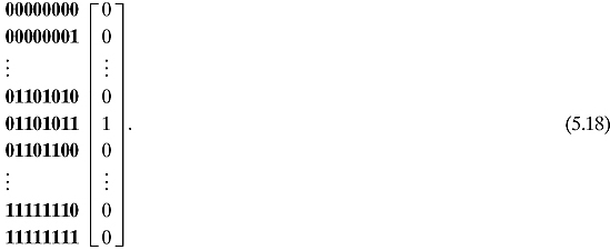
We can describe our byte in yet another way: as a 28 = 256 row vector
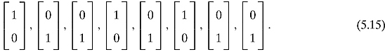
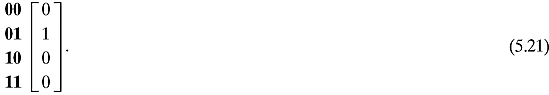
Exercise 5.1.3 Express the three bits 101 or ![]() as a vector in
as a vector in ![]() . Do the same for 011 and 111.
. Do the same for 011 and 111.
![]()
This is fine for the classical world. However, for the quantum world, in order to permit superposition, a generalization is needed: every state of an eight-qubit system can be written as
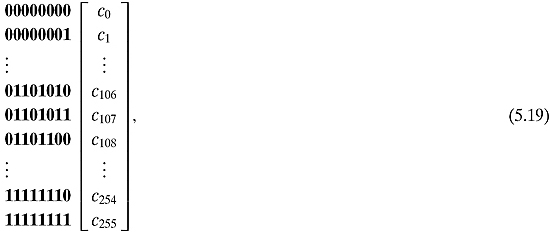
where ![]() . Eight qubits together is called a qubyte.
. Eight qubits together is called a qubyte.
In the classical world, it is necessary to indicate the state of each bit of a byte. This amounts to writing eight bits. In the quantum world, a state of eight qubits is given by writing 256 complex numbers. As we stated in Section 3.4, this exponential growth was one of the reasons researchers started giving thought to the notion of quantum computing. If one wanted to emulate a quantum computer with a 64-qubit register, one would need to store 264 = 18, 446,744, 073, 709, 551, 616 complex numbers. This is way beyond our current storage capability.
Let us practice writing two qubits in ket notation. A qubit pair can be written as
![]()
which means that the first qubit is in state ![]() and the second qubit is in state
and the second qubit is in state ![]() . Because the tensor product is understood, we might also denote these qubits as
. Because the tensor product is understood, we might also denote these qubits as ![]() ,
, ![]() , or
, or ![]() . Yet another way to look at these two qubits as the 4-by-1 matrix is
. Yet another way to look at these two qubits as the 4-by-1 matrix is
Exercise 5.1.4 What vector corresponds to the state ![]() ?
?
Example 5.1.2 The qubit corresponding to
can be written as
![]()
![]()
A general state of a two-qubit system can be written as
![]()
The tensor product of two states is not commutative:

The left ket describes the state in which the first qubit is in state 0 and the second qubit is in state 1. The right ket indicates that first qubit is in state 1 and the second qubit is in state 0.
Let us briefly revisit the notion of entanglement again. If the system is in the state
![]()
then that means that the the two qubits are entangled. That is, if we measure the first qubit and it is found in state ![]() then we automatically know that the state of the second qubit is
then we automatically know that the state of the second qubit is ![]() . Similarly, if we measure the first qubit and find it in state
. Similarly, if we measure the first qubit and find it in state ![]() then we know the second qubit is also in state
then we know the second qubit is also in state ![]() .
.
5.2 CLASSICAL GATES
Classical logical gates are ways of manipulating bits. Bits enter and exit logical gates. We will need ways of manipulating qubits and will study classical gates from the point of view of matrices. As stated in Section 5.1, we represent n input bits as a 2n-by-1 matrix and m output bits as a 2m-by-1 matrix. How should we represent our logical gates? When one multiplies a 2m-by-2n matrix with a 2n-by-1 matrix, the result is a 2m-by-1 matrix. In symbols:
![]()
So bits will be represented by column vectors and logic gates by matrices.
Let us try a simple example. Consider the NOT gate.

NOT takes as input one bit, or a 2-by-1 matrix, and outputs one bit, or a 2-by-1 matrix. NOT of ![]() equals
equals ![]() and NOT of
and NOT of ![]() equals
equals ![]() . Consider the matrix
. Consider the matrix
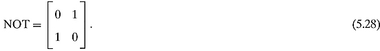
This matrix satisfies
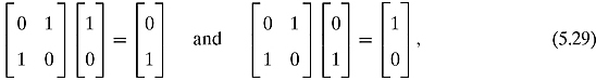
which is exactly what we want.
What about the other gates? Consider the AND gate. The AND gate is different from the NOT gate because AND accepts two bits and outputs one bit.

Because there are two inputs and one output, we will need a 21-by-22 matrix. Consider the matrix
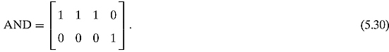
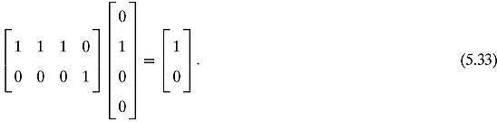
This matrix satisfies

We can write this as
![]()
In contrast, consider another 4-by-1 matrix:
We can write this as
![]()
Exercise 5.2.1 Calculate ![]() .
.
![]()
What would happen if we put an arbitrary 4-by-1 matrix to the right of AND?
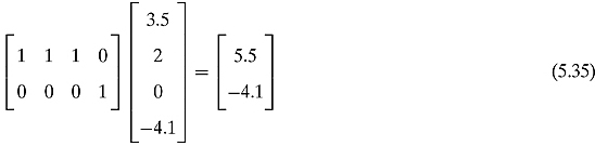
This is clearly nonsense. We are allowed only to multiply these classical gates with vectors that represent classical states, i.e., column matrices with a single 1 entry and all other entries 0. In the classical world, the bits are in only one state at a time and are described by such vectors. Only later, when we delve into quantum gates, will we have more room (and more fun).
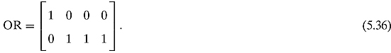
The OR gate
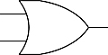
can be represented by the matrix
Exercise 5.2.2 Show that this matrix performs the OR operation.
![]()
The NAND gate
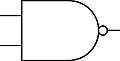
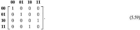
is of special importance because every logical gate can be composed of NAND gates. Let us try to determine which matrix would correspond to NAND. One way is to sit down and consider for which of the four possible input states of two bits (00, 01, 10, 11) does NAND output a 1 (answer: 00, 01, 10), and in which states does NAND output a 0 (answer: 11). From this, we realize that NAND can be written as
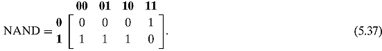
Notice that the column names correspond to the inputs and the row names correspond to the outputs. 1 in the jth column and ith row means that on entry j the matrix/gate will output i.
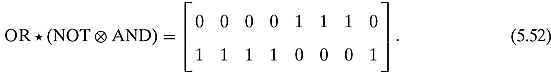
There is, however, another way in which one can determine the NAND gate. The NAND gate is really the AND gate followed by the NOT gate.
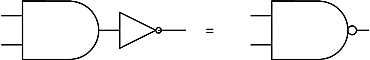
In other words, we can perform the NAND operation by first performing the AND operation and then the NOT operation. In terms of matrices we can write this as
Exercise 5.2.3 Find a matrix that corresponds to NOR.
![]()
This way of thinking of NAND brings to light a general situation. When we perform a computation, we often have to carry out one operation followed by another.
![]()
We call this procedure performing sequential operations. If matrix A corresponds to performing an operation and matrix B corresponds to performing another operation, then the matrix B * A corresponds to performing the operation sequentially. Notice that B * A looks like the reverse of our picture which has, from left to right, A and then B. Do not be alarmed by this. The reason for this is because we read from left to right and hence we depict processes as flowing from left to right. We could have easily drawn the above figure as

with no confusion.1 We shall follow the convention that computation flows from left to right and omit the heads of the arrows. And so a computation of A followed by B shall be denoted

Let us be formal with the number of inputs and the number of outputs. If A is an operation with m input bits and n output bits, then we shall draw this as

The matrix A will be of size 2n-by-2m. Say, B takes the n outputs of A as input and outputs p bits, i.e.,
![]()
then B is represented by a 2p-by-2n matrix B, and performing one operation sequentially followed by another operation corresponds to B *A, which is a (2p-by-2n) * (2n-by-2m)=(2p-by-2m) matrix.
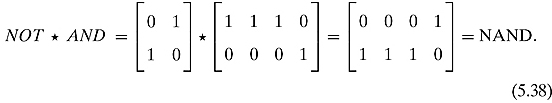
Besides sequential operations, there are parallel operations as well.
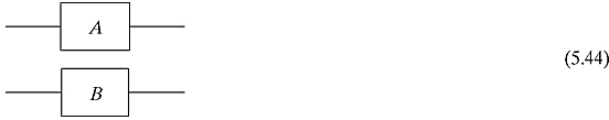
Here we have A acting on some bits and B on others. This will be represented by ![]() (see Section 2.7). Let us be exact with the number of inputs and the number of outputs.
(see Section 2.7). Let us be exact with the number of inputs and the number of outputs.
A will be of size 2n-by-2m. B will be of size 2n′-by-2m′. Following Equation (2.174) in Section 2.7, ![]() is of size 2n2n′ = 2n + n′-by- 2m2m′ =2m + m′.
is of size 2n2n′ = 2n + n′-by- 2m2m′ =2m + m′.
Exercise 5.2.4 In Exercise 2.7.4, we proved that ![]() . What does this fact correspond to in terms of performing parallel operations on different bits?
. What does this fact correspond to in terms of performing parallel operations on different bits?
![]()
Combinations of sequential and parallel operations gates/matrices will be called circuits. We will, of course, construct some really complicated matrices, but they will all be decomposable into the sequential and parallel compositions of simple gates.
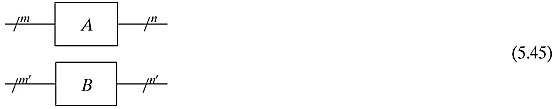
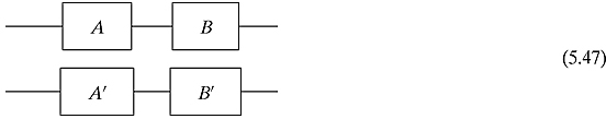
Exercise 5.2.5 In Exercise 2.7.9, we proved that for matrices of the appropriate sizes A, A′, B, and B′ we have the following equation:
![]()
To what does this correspond in terms of performing different operations on different (qu) bits? (Hint: Consider the following figure.)
![]()
Example 5.2.1 Let A be an operation that takes n inputs and gives m outputs. Let B take p < m of these outputs and leave the other m− p outputs alone. B outputs q bits.
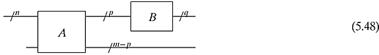
A is a 2m-by-2n matrix. B is a 2q-by-2p matrix. As nothing should be done to the m− p bits, we might represent this as the 2m−p-by-2m−p identity matrix Im−p. We do not draw any gate for the identity matrix. The entire circuit can be represented by the following matrix:
![]()
![]()
Example 5.2.2 Consider the circuit.
This is represented by
![]()
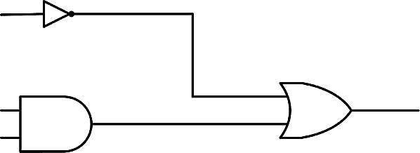
Let us see how the operations look like as matrices. Calculating, we get
And so we get
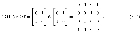
Let us see if we can formulate DeMorgan’s laws in terms of matrices. One of DeMorgan's laws states that ![]() . Here is a pictorial representation.
. Here is a pictorial representation.
![]()

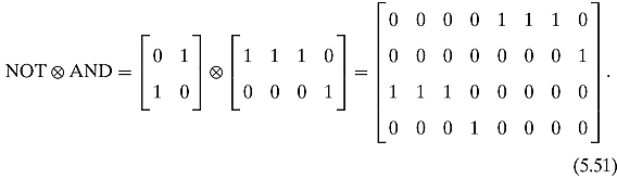
In terms of matrices this corresponds to
![]()
First, let us calculate the tensor product:
This DeMorgan’s law corresponds to the following identity of matrices:
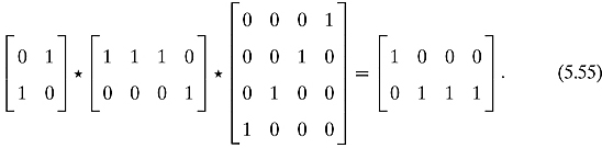
Exercise 5.2.6 Multiply out these matrices and confirm the identity.
![]()
Exercise 5.2.7 Formulate the other DeMorgan’s law
![]()
in terms of matrices.
![]()
Exercise 5.2.8 Write the matrix that would correspond to a one-bit adder. A one-bit adder adds the bits x, y, and c (a carry-bit from an earlier adder) and outputs the bits z and c′ (a carry-bit for the next adder). There are three inputs and two outputs, so the matrix will be of dimension 22-by-23. (Hint: Mark the columns as 000, 001, 010,…,110, 111, where column, say, 101 corresponds to x = 1, y = 0, c = 1. Mark the rows as 00, 01, 10, 11, where row, say, 10, corresponds to z = 1, c′ = 0. When x = 1, y = 0, c = 1, the output should be z = 0 and c′ = 1. So place a 1 in the row marked 01 and a 0 in all other rows.)
![]()
Exercise 5.2.9 In Exercise 5.2.8, you determined the matrix that corresponds to a one-bit adder. Check that your results are correct by writing the circuit in terms of classical gates and then converting the circuit to a big matrix.
![]()
5.3 REVERSIBLE GATES
Not all the logical gates that we dealt with in Section 5.2 will work in quantum computers. In the quantum world, all operations that are not measurements are reversible and are represented by unitary matrices. The AND operation is not reversible. Given an output of ![]() from AND, one cannot determine if the input was
from AND, one cannot determine if the input was ![]() ,
, ![]() , or
, or ![]() . So from an output of the AND gate, one cannot determine the input and hence AND is not reversible. In contrast, the NOT gate and the identity gates are reversible. In fact, they are their own inverses:
. So from an output of the AND gate, one cannot determine the input and hence AND is not reversible. In contrast, the NOT gate and the identity gates are reversible. In fact, they are their own inverses:
![]()
Reversible gates have a history that predates quantum computing. Our everyday computers lose energy and generate a tremendous amount of heat. In the 1960s, Rolf Landauer analyzed computational processes and showed that erasing information, as opposed to writing information, is what causes energy loss and heat. This notion has come to be known as the Landauer’s principle.
In order to gain a real-life intuition as to why erasing information dissipates energy, consider a tub of water with a wall separating the two sides as in Figure 5.1.
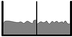
Figure 5.1. Tub with water in no state.
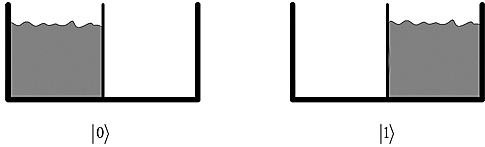
Figure 5.2. Tub with water in state ![]() and state
and state ![]() .
.
This tub is used as a way of storing a bit of information. If all the water is pushed to the left then the system is in state ![]() , and if all the water is pushed to the right then the system is in state
, and if all the water is pushed to the right then the system is in state ![]() , as in Figure 5.2.
, as in Figure 5.2.
What would correspond to erasing information in such a system? If there were a hole in the wall separating the 0 and 1 regions, then the water could seep out and we would not know what state the system would be in. One can easily place a turbine where the water is seeping out (see Figure 5.3) and generate energy. Hence, losing information means energy is being dissipated.
Notice, also, that writing information is a reversible procedure. If the tub is in no state and we push all the water to the left and set the water to state ![]() , all one needs to do is remove the wall and the water will go into both regions resulting in no state. This is shown in Figure 5.4. We have reversed the fact that information was written. In contrast, erasing information is not reversible. Start at state
, all one needs to do is remove the wall and the water will go into both regions resulting in no state. This is shown in Figure 5.4. We have reversed the fact that information was written. In contrast, erasing information is not reversible. Start at state ![]() , and then remove the wall that separates the two parts of the tub. That is erasing the information. How could we return to the original state? There are two possible states to return to, as in Figure 5.5.
, and then remove the wall that separates the two parts of the tub. That is erasing the information. How could we return to the original state? There are two possible states to return to, as in Figure 5.5.
The obvious answer is that we should push all the water back to state ![]() . But the only way we know that
. But the only way we know that ![]() is the original state is if that information is copied to the brain. In that case, the system is both the tub and the brain, and we did not really erase the fact that state
is the original state is if that information is copied to the brain. In that case, the system is both the tub and the brain, and we did not really erase the fact that state ![]() was the original state. Our brain was still storing the information.
was the original state. Our brain was still storing the information.
Let us reexamine this intuition by considering two people, Alice and Bob. If Alice writes a letter on an empty blackboard and then Bob walks into the room, he can then erase the letter that Alice wrote on the board and return the blackboard into its original pristine state. Thus, writing is reversible. In contrast, if there is a board with writing on it and Alice erases the board, then when Bob walks into the room he cannot write what was on the board. Bob does not know what was on the board before Alice erased it. So Alice’s erasing was not reversible.
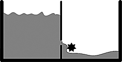
Figure 5.3. State ![]() dissipating and creating energy.
dissipating and creating energy.
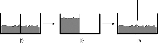
Figure 5.4. Reversibility of writing.
We have found that erasing information is an irreversible, energy-dissipating operation. In the 1970s, Charles H. Bennett continued along these lines of thought. If erasing information is the only operation that uses energy, then a computer that is reversible and does not erase would not use any energy. Bennett started working on reversible circuits and programs.
What examples of reversible gates are there? We have already seen that the identity gate and NOT gates are reversible. What else is there? Consider the following controlled-NOT gate:
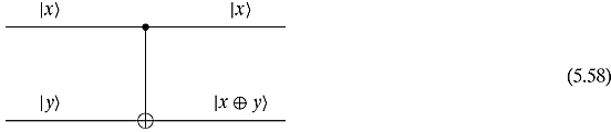
This gate has two inputs and two outputs. The top input is the control bit. It controls what the output will be. If ![]() , then the bottom output of
, then the bottom output of ![]() will be the same as the input. If
will be the same as the input. If ![]() , then the bottom output will be the opposite. If we write the top qubit first and then the bottom qubit, then the controlled-NOT gate takes
, then the bottom output will be the opposite. If we write the top qubit first and then the bottom qubit, then the controlled-NOT gate takes ![]() to
to ![]() , where
, where ![]() is the binary exclusive or operation.
is the binary exclusive or operation.

Figure 5.5. Irreversibility of erasing.
The matrix that corresponds to this reversible gate is
The controlled-NOT gate can be reversed by itself. Consider the following figure:
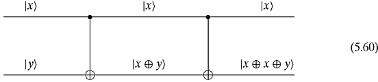
State ![]() goes to
goes to ![]() , which further goes to
, which further goes to ![]() . This last state is equal to
. This last state is equal to ![]() because
because ![]() is associative. Because
is associative. Because ![]() is always equal to 0, this state reduces to the original
is always equal to 0, this state reduces to the original ![]() .
.
Exercise 5.3.1 Show that the controlled-NOT gate is its own inverse by multiplying the corresponding matrix by itself and arriving at the identity matrix.
![]()
An interesting reversible gate is the Toffoli gate:
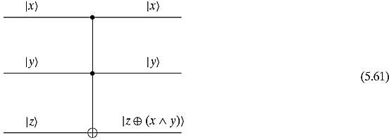
This is similar to the controlled-NOT gate, but with two controlling bits. The bottom bit flips only when both of the top two bits are in state ![]() . We can write this operation as taking state
. We can write this operation as taking state ![]() to
to ![]() .
.
Exercise 5.3.2 Show that the Toffoli gate is its own inverse.
![]()
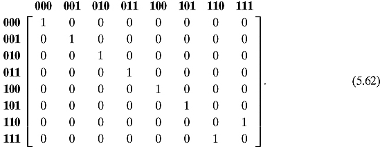
The matrix that corresponds to this gate is
Example 5.3.1 The NOT gate has no controlling bit, the controlled-NOT gate has one controlling bit, and the Toffoli gate has two controlling bits. Can we go on with this? Yes. A gate with three controlling bits can be constructed from three Toffoli gates as follows:

![]()
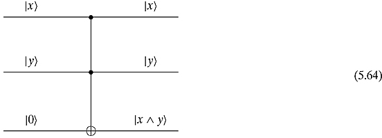
One reason why the Toffoli gate is interesting is that it is universal. In other words, with copies of the Toffoli gate, you can make any logical gate. In particular, you can make a reversible computer using only Toffoli gates. Such a computer would, in theory, neither use any energy nor give off any heat.
In order to see that the Toffoli gate is universal, we will show that it can be used to make both the AND and NOT gates. The AND gate is obtained by setting the bottom ![]() input to
input to ![]() . The bottom output will then be
. The bottom output will then be ![]() .
.
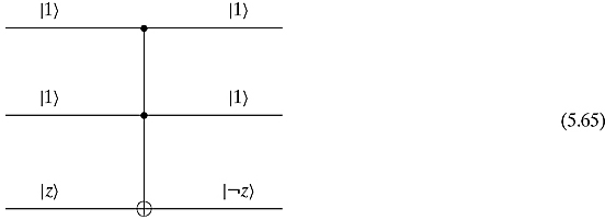
The NOT gate is obtained by setting the top two inputs to ![]() . The bottom output will be
. The bottom output will be ![]() .
.
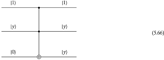
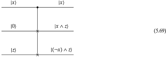
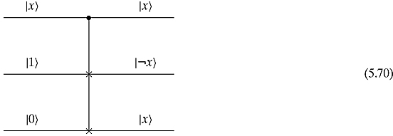
In order to construct all gates, we must also have a way of producing a fanout of values. In other words, a gate is needed that inputs a value and outputs two of the same values. This can be obtained by setting ![]() to
to ![]() and
and ![]() to
to ![]() . This makes the output
. This makes the output ![]() .
.
Exercise 5.3.3 Construct the NAND with one Toffoli gate. Construct the OR gate with two Toffoli gates.
![]()
Another interesting reversible gate is the Fredkin gate. The Fredkin gate also has three inputs and three outputs.
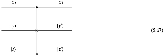
The top ![]() input is the control input. The output is always the same
input is the control input. The output is always the same ![]() . If
. If ![]() is set to
is set to ![]() , then
, then ![]() and
and ![]() , i.e., the values stay the same. If, on the other hand, the control
, i.e., the values stay the same. If, on the other hand, the control ![]() is set to
is set to ![]() then the outputs are reversed:
then the outputs are reversed: ![]() and
and ![]() . In short,
. In short, ![]() and
and ![]() .
.
Exercise 5.3.4 Show that the Fredkin gate is its own inverse.
![]()
The matrix that corresponds to the Fredkin gate is

The Fredkin gate is also universal. By setting ![]() to
to ![]() , we get the AND gate as follows:
, we get the AND gate as follows:
The NOT gate and the fanout gate can be obtained by setting ![]() to
to ![]() and
and ![]() to
to ![]() . This gives us
. This gives us
So both the Toffoli and the Fredkin gates are universal. Not only are both reversible gates; a glance at their matrices indicates that they are also unitary. In the next section, we look at other unitary gates.
5.4 QUANTUM GATES
Definition 5.4.1 A quantum gate is simply an operator that acts on qubits. Such operators will be represented by unitary matrices.
We have already worked with some quantum gates such as the identity operator I, the Hadamard gate H, the NOT gate, the controlled-NOT gate, the Toffoli gate, and the Fredkin gate. What else is there?
Let us look at some other quantum gates. The following three matrices are called Pauli matrices and are very important:

They occur everywhere in quantum mechanics and quantum computing.2 Note that the X matrix is nothing more than our NOT matrix. Other important matrices that will be used are
Exercise 5.4.1 Show that each of these matrices are unitary.
![]()
Exercise 5.4.2 Show the action of each of these matrices on an arbitrary qubit [c0, c1]T.
![]()
Exercise 5.4.3 These operations are intimately related to each other. Prove the following relationships between the operations:
(i) X2 = Y2 = Z2 = I,
(ii) ![]() ,
,
(iii) X = HZH,
(iv) Z = HXH,
(v) −1Y = HYH,
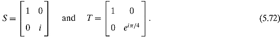
(vi) S = T2,
(vii) −1Y = XYX.
![]()
There are still other quantum gates. Let us consider a one-qubit quantum gate with an interesting name. The gate is called the square root of NOT and is denoted ![]() . The matrix representation of this gate is
. The matrix representation of this gate is

The first thing to notice is that this gate is not its own inverse, that is,
![]()
In order to understand why this gate has such a strange name, let us multiply ![]() by itself:
by itself:

which is very similar to the NOT gate. Let us put the qubits ![]() and
and ![]() through
through ![]() gate twice. We get
gate twice. We get
![]()
and
![]()
Remembering that ![]() and
and ![]() both represent the same state, we are confident in saying that the square of
both represent the same state, we are confident in saying that the square of ![]() performs the same operation as the NOT gate, and hence the name.
performs the same operation as the NOT gate, and hence the name.
There is one other gate we have not discussed: the measurement operation. This is not unitary or, in general, even reversible. This operation is usually performed at the end of a computation when we want to measure qubits (and find bits). We shall denote it as
![]()
There is a beautiful geometric way of representing one-qubit states and operations. Remember from Chapter 1, page 18, that for a given complex number c = x + yi whose modulus is 1, there is a nice way of visualizing c as an arrow of length 1 from the origin to the circle of radius 1.
![]()
In other words, every complex number of radius 1 can be identified by the angle ![]() that the vector makes with the positive x axis.
that the vector makes with the positive x axis.
There is an analogous representation of a qubit as an arrow from the origin to a three-dimensional sphere. Let us see how it works. A generic qubit is of the form
![]()
where |c0|2 + |c1|2 = 1. Although at first sight there are four real numbers involved in the qubit given in Equation (5.80), it turns out that there are only two actual degrees of freedom to the three-dimensional ball (as latitude and longitude on the Earth). Let us rewrite the qubit in Equation (5.80) in polar form:
![]()
and
![]()
and so Equation (5.80) can be rewritten as
![]()
There are still four real parameters: r0, r1, ![]() ,
, ![]() . However, a quantum physical state does not change if we multiply its corresponding vector by an arbitrary complex number (of norm 1, see Chapter 4, page 109). We can therefore obtain an equivalent expression for the qubit in Equation (5.80), where the amplitude for
. However, a quantum physical state does not change if we multiply its corresponding vector by an arbitrary complex number (of norm 1, see Chapter 4, page 109). We can therefore obtain an equivalent expression for the qubit in Equation (5.80), where the amplitude for ![]() is real, by “killing” its phase:
is real, by “killing” its phase:
![]()
We now have only three real parameters, namely, r0, r1, and ![]() . But we can do better: using the fact that
. But we can do better: using the fact that
![]()
we get that
![]()
We can rename them as
![]()
Summing up, the qubit in Equation (5.80) is now in the canonical representation
![]()
with only two real parameters remaining.
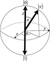
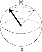
Figure 5.6. Bloch sphere.
What is the range of the two angles θ and ![]() ? We invite you to show that
? We invite you to show that ![]() 2π and 0
2π and 0 ![]() are enough to cover all possible qubits.
are enough to cover all possible qubits.
Exercise 5.4.4 Prove that every qubit in the canonical representation given in Equation (5.88) with ![]() is equivalent to another one where θ lies in the first quadrant of the plane. (Hint: Use a bit of trigonometry and change
is equivalent to another one where θ lies in the first quadrant of the plane. (Hint: Use a bit of trigonometry and change ![]() according to your needs.)
according to your needs.)
![]()
As only two real numbers are necessary to identify a qubit, we can map it to an arrow from the origin to the three-dimensional sphere of ![]() of radius 1 known as the Bloch sphere, as shown in Figure 5.6.
of radius 1 known as the Bloch sphere, as shown in Figure 5.6.
Every qubit can be represented by two angles that describe such an arrow. The two angles will correspond to the latitude (θ) and the longitude ![]() needed to specify any position on Earth. The standard parametrization of the unit sphere is
needed to specify any position on Earth. The standard parametrization of the unit sphere is
![]()
![]()
![]()
where ![]() and 0≤ θ ≤ π.
and 0≤ θ ≤ π.
However, there is a caveat: suppose we use this representation to map our qubit on the sphere. Then, the points (θ, ![]() ) and (π − θ,
) and (π − θ, ![]() ) represent the same qubit, up to the factor−1. Conclusion: the parametrization would map the same qubit twice, on the upper hemisphere and on the lower one. To mitigate this problem, we simply double the “latitude” to cover the entire sphere at “half speed”:
) represent the same qubit, up to the factor−1. Conclusion: the parametrization would map the same qubit twice, on the upper hemisphere and on the lower one. To mitigate this problem, we simply double the “latitude” to cover the entire sphere at “half speed”:
![]()
![]()
![]()
Let us spend a few moments familiarizing ourselves with the Bloch sphere and its geometry. The north pole corresponds to the state ![]() and the south pole corresponds to the state
and the south pole corresponds to the state ![]() . These two points can be taken as the geometrical image of the good old-fashioned bit. But there are many more qubits out there, and the Bloch sphere clearly shows it.
. These two points can be taken as the geometrical image of the good old-fashioned bit. But there are many more qubits out there, and the Bloch sphere clearly shows it.
The precise meaning of the two angles in Equation (5.88) is the following: ![]() is the angle that
is the angle that ![]() makes from x along the equator and θ is half the angle that
makes from x along the equator and θ is half the angle that ![]() makes with the x axis.
makes with the x axis.
When a qubit is measured in the standard basis, it collapses to a bit, or equivalently, to the north or south pole of the Bloch sphere. The probability of which pole the qubit will collapse to depends exclusively on how high or low the qubit is pointing, i.e., to its latitude. In particular, if the qubit happens to be on the equator, there is a 50–50 chance of it collapsing to either ![]() or
or ![]() . As the angle θ expresses the qubit’s latitude, it controls its chance of collapsing north or south.
. As the angle θ expresses the qubit’s latitude, it controls its chance of collapsing north or south.
Exercise 5.4.5 Consider a qubit whose θ is equal to ![]() . Change it to
. Change it to ![]() and picture the result. Then compute its likelihood of collapsing to the south pole after being observed.
and picture the result. Then compute its likelihood of collapsing to the south pole after being observed.
![]()
Take an arbitrary arrow and rotate it around the z axis; in the geographical metaphor, you are changing its longitude:
Notice that the probability of which classical state it will collapse to is not affected. Such a state change is called a phase change. In the representation given in Equation (5.88), this corresponds to altering the phase parameter ![]() .
.
Before we move on, one last important item: just as ![]() and
and ![]() sit on opposite sides of the sphere, so an arbitrary pair of orthogonal qubits is mapped to antipodal points of the Bloch sphere.
sit on opposite sides of the sphere, so an arbitrary pair of orthogonal qubits is mapped to antipodal points of the Bloch sphere.
Exercise 5.4.6 Show that if a qubit has latitude 2θ and longitude ![]() on the sphere, its orthogonal lives in the antipode π −2θ and
on the sphere, its orthogonal lives in the antipode π −2θ and ![]() .
.
![]()
That takes care of states of a qubit. What about the dynamics? The Bloch sphere is interesting in that every unitary 2-by-2 matrix (i.e., a one-qubit operation) can be visualized as a way of manipulating the sphere. We have seen in Chapter 2, page 66, that every unitary matrix is an isometry. This means that such a matrix maps qubits to qubits and the inner product is preserved. Geometrically, this corresponds to a rotation or an inversion of the Bloch sphere.
The X, Y, and Z Pauli matrices are ways of “flipping” the Bloch sphere 180º about the x, y, and z axes respectively. Remember that X is nothing more than the NOT gate, and takes ![]() to
to ![]() and vice versa. But it does more; it takes everything above the equator to below the equator. The other Pauli matrices work similarly. Figure 5.7 shows the action of the Y operation.
and vice versa. But it does more; it takes everything above the equator to below the equator. The other Pauli matrices work similarly. Figure 5.7 shows the action of the Y operation.

Figure 5.7. A rotation of the Bloch sphere at y.
There are times when we are not interested in performing a total 180° flip but just want to turn the Bloch sphere 0 degrees along a particular direction.
The first such gates are the phase shift gates. It is defined as
This gate performs the following operation on an arbitrary qubit:
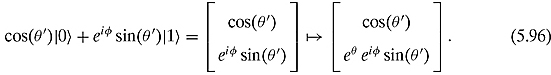
This corresponds to a rotation that leaves the latitude alone and just changes the longitude. The new state of the qubit will remain unchanged. Only the phase will change.
There are also times when we want to rotate a particular number of degrees around the x, y, or z axis. These three matrices will perform the task:
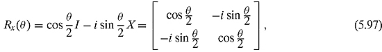
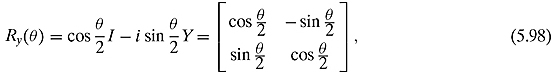

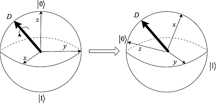
Figure 5.8. A rotation of the Bloch sphere at y.
There are rotations around axes besides the x, y, and z axes. Let D =(Dx, Dy, Dz) be a three-dimensional vector of size 1 from the origin. This determines an axis of the Bloch sphere around which we can spin (see Figure 5.8). The rotation matrix is given as
![]()
As we have just seen, the Bloch sphere is a very valuable tool when it comes to understanding qubits and one-qubit operations. What about n-qubits? It turns out there is a higher-dimensional analog of the sphere, but coming to grips with it is not easy. Indeed, it is a current research challenge to develop new ways of visualizing what happens when we manipulate several qubits at once. Entanglement, for instance, lies beyond the scope of the Bloch sphere (as it involves at least two qubits).
There are still other quantum gates. One of the central features of computer science is an operation that is done only under certain conditions and not under others. This is equivalent to an IF-THEN statement. If a certain (qu)bit is true, then a particular operation should be performed, otherwise the operation is not performed. For every n-qubit unitary operation U, we can create a unitary (n+ 1)-qubit operation controlled-U or CU.
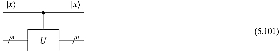
This operation will perform the U operation if the top ![]() input is a
input is a ![]() and will simply perform the identity operation if
and will simply perform the identity operation if ![]() is
is ![]() .
.
For the simple case of
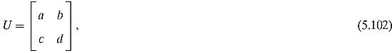
the controlled-U operation can be seen to be
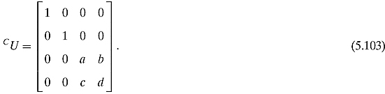
This same construction works for matrices larger than 2-by-2.
Exercise 5.4.7 Show that the constructed CU works as it should when the top qubit is set to ![]() or set to
or set to ![]() .
.
![]()
Exercise 5.4.8 Show that if U is unitary, then so is CU.
![]()
Exercise 5.4.9 Show that the Toffoli gate is nothing more than C(CNOT).
![]()
It is well known that every logical circuit can be simulated using only the AND gate and the NOT gate. We say that {AND, NOT} forms a set of universal logical gates. The NAND gate by itself is also a universal logical gate. We have also seen in Section 5.3 that both the Toffoli gate and the Fredkin gate are each universal logic gates. This leads to the obvious question: are there sets of quantum gates that can simulate all quantum gates? In other words, are there universal quantum gates? The answer is yes.3 One set of universal quantum gates is
![]()
that is, the Hadamard gate, the controlled-NOT gate, and this phase shift gate.
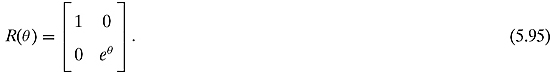
There is also a quantum gate called the Deutsch gate, D(θ), depicted as
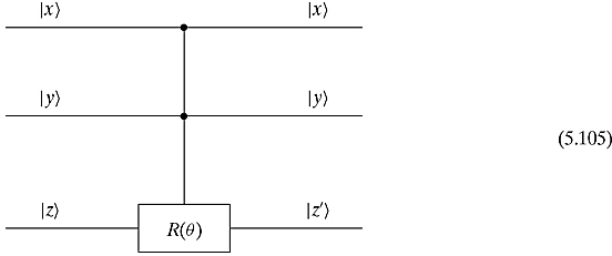
which is very similar to the Toffoli gate. If the inputs ![]() and
and ![]() are both
are both ![]() , then the phase shift operation R(θ) will act on the
, then the phase shift operation R(θ) will act on the ![]() input. Otherwise, the
input. Otherwise, the ![]() will simply be the same as the
will simply be the same as the ![]() . When θ is not a rational multiple of π, D(θ) by itself is a universal three-qubit quantum gate. In other words, D(θ) will be able to mimic every other quantum gate.
. When θ is not a rational multiple of π, D(θ) by itself is a universal three-qubit quantum gate. In other words, D(θ) will be able to mimic every other quantum gate.
Exercise 5.4.10 Show that the Toffoli gate is nothing more than ![]() .
.
![]()
Throughout the rest of this text, we shall demonstrate many of the operations that can be performed with quantum gates. However, there are limitations to what can be done with them. For one thing, every operation must be reversible. Another limitation is a consequence of the the No-Cloning Theorem. This theorem says that it is impossible to clone an exact quantum state. In other words, it is impossible to make a copy of an arbitrary quantum state without first destroying the original. In “computerese,” this says that we can “cut” and “paste” a quantum state, but we cannot “copy” and “paste” it. “Move is possible. Copy is impossible.”
What is the difficulty? How would such a cloning operation look? Let ![]() represent a quantum system. As we intend to clone states in this system, we shall “double” this vector space and deal with
represent a quantum system. As we intend to clone states in this system, we shall “double” this vector space and deal with ![]() . A potential cloning operation would be a linear map (indeed unitary!)
. A potential cloning operation would be a linear map (indeed unitary!)
![]()
that should take an arbitrary state ![]() in the first system and, perhaps, nothing in the second system and clone
in the first system and, perhaps, nothing in the second system and clone ![]() , i.e.,
, i.e.,
![]()
This seems like a harmless enough operation, but is it? If C is a candidate for cloning, then certainly on the basic states
![]()
Because C must be linear, we should have that
![]()
for an arbitrary quantum state, i.e., an arbitrary superposition of ![]() and
and ![]() . Suppose we start with
. Suppose we start with ![]() . Cloning such a state would mean that
. Cloning such a state would mean that
![]()
However, if we insist that C is a quantum operation, then C must be linear,4 and hence, must respect the addition and the scalar multiplication in ![]() . If C was linear, then
. If C was linear, then
But
![]()
So C is not a linear map,5 and hence is not permitted.
In contrast to cloning, there is no problem transporting arbitrary quantum states from one system to another. Such a transporting operation would be a linear map
![]()
that should take an arbitrary state ![]() in the first system and, say, nothing in the second system, and transport
in the first system and, say, nothing in the second system, and transport ![]() to the second system, leaving nothing in the first system, i.e.,
to the second system, leaving nothing in the first system, i.e.,
![]()
We do not run into the same problem as earlier if we transport a superposition of states. In detail,

This is exactly what we would expect from a transporting operation.6
Fans of Star Trek have long known that when Scotty “beams” Captain Kirk down from the Starship Enterprise to the planet Zygon, he is transporting Captain Kirk to Zygon. The Kirk of the Enterprise gets destroyed and only the Zygon Kirk survives. Captain Kirk is not being cloned. He is being transported. (Would we really want many copies of Captain Kirk all over the Universe?)
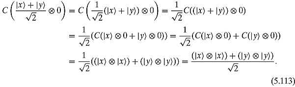
The reader might see an apparent contradiction in what we have stated. On the one hand, we have stated that the Toffoli and Fredkin gates can mimic the fanout gate. The matrices for the Toffoli and Fredkin gates are unitary, and hence they are quantum gates. On the other hand, the no-cloning theorem says that no quantum gates can mimic the fanout operation. What is wrong here? Let us carefully examine the Fredkin gate. We have seen how this gate performs the cloning operation
![]()
However, what would happen if the x input was in a superposition of states say, ![]() , while leaving y = 1 and z = 0. This would correspond to the state
, while leaving y = 1 and z = 0. This would correspond to the state

Multiplying this state with the Fredkin gate gives us
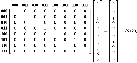
The resulting state is
![]()
So, whereas on a classical bit x, the Fredkin gate performs the fanout operation, on a superposition of states the Fredkin gate performs the following very strange operation:
![]()
This strange operation is not a fanout operation. Thus, the no-cloning theorem safely stands.
Exercise 5.4.11 Do a similar analysis for the Toffoli gate. Show that the way we set the Toffoli gate to perform the fanout operation does not clone a superposition of states.
![]()
Reader Tip. The no-cloning theorem is of major importance in Chapter 9. ![]()
References: The basics of qubits and quantum gates can be found in any textbook on quantum computing. They were first formulated by David Deutsch in 1989 (Deutsch, 1989).
Section 5.2 is simply a reformulation of basic computer architecture in terms of matrices.
The history of reversible computation can be found in Bennett (1988). The readable article (Landauer, 1991) by one of the forefathers of reversible computation is strongly recommended.
The no-cloning theorem was first proved in Dieks (1982) and Wootters and Zurek (1982).
1 If the text were written in Arabic or Hebrew, this problem would not even arise.
2 Sometimes the notation σx, σy, and σz is used for these matrices.
3 We must clarify what we mean by “simulate.” In the classical world, we say that one circuit Circ simulates another circuit Circ′ if for any possible inputs, the output for Circ will be the same for Circ′. Things in the quantum world are a tad more complicated. Because of the probabilistic nature of quantum computation, the outputs of a circuit are always probabilistic. So we have to reformulate what we mean when we talk about simulate. We shall not worry about this here.
4 Just a reminder: C being linear means that
![]()
and
![]()
5 C is, however, a legitimate set map.
6 In fact, we will show how to transport arbitrary quantum states at the end of Chapter 9.