Appendix B
Answers to Selected Exercises
CHAPTER 1
![]()
As neither of the factors have real solutions, there are no real solutions to the entire equation.
Ex. 1.1.2: − i.
Ex. 1.1.3: −1 −3i; −2 + 14i.
Ex. 1.1.4: Simply multiply out ( −1 + i)2 +2( −1 + i) + 2 and show that it equals 0.
Ex. 1.2.1: ( −5, 5).
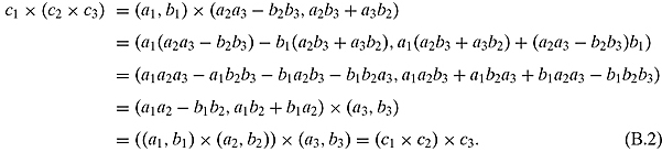
Ex. 1.2.2: Setting c1 = (a1, b1), c2 = (a2, b2), and c3 = (a3, b3). Then we have
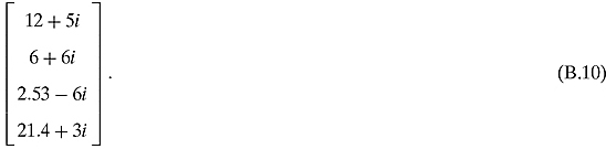
Ex. 1.2.3: ![]() .
.
Ex. 1.2.4: 5.
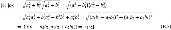
Ex. 1.2.5: Setting c1 = (a1, b1) and c2 = (a2, b2). Then
Ex. 1.2.6: This can be carried out algebraically like Exercise 1.2.5. One should also think of this geometrically after reading Section 1.3. Basically this says that any side of a triangle is not greater than the sum of the other two sides.
Ex. 1.2.7: Examine it!
Ex. 1.2.8: Too easy.
Ex. 1.2.9: (a1, b1)(−1, 0) = (−1a1 − 0b1, 0a1 − 1b1) = (−a1, −b1).
Ex. 1.2.10: Setting c1 = (a1, b1) and c2 = (a2, b2). Then
![]()
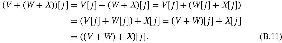
Ex. 1.2.11: Setting c1 = (a1, b1) and c2 = (a2, b2). Then
![]()
![]()
Ex. 1.2.12: Although the map is bijective, it is not a field isomorphism because it does not respect the multiplication, i.e., in general,
![]()
Ex. 1.3.1: 3 + 0i.
Ex. 1.3.2: 1 − 2i.
Ex. 1.3.3: 1.5 + 2.6i.
Ex. 1.3.4: 5i.
Ex. 1.3.5: If c = a + bi, the effect of multiplying by r0 is just r0a + r0bi. The vector in the plane has been stretched by the constant factor r0. You can see it better in polar coordinates: only the magnitude of the vector has changed, the angle stays the same. The effect on the plane is an overall dilation by r0, and no rotation.
Ex. 1.3.6: The best way to grasp this exercise it to pass to the polar representation: let c = (ρ, θ) and c0 = (ρ0, θ0). Their product is (ρρ0, θ + θ0). This is true for all c. The plane has been dilated by the factor ρ0 and rotated by the angle θ0.
Ex. 1.3.7: 2i.
Ex. 1.3.8: (1−i)5 = −4 + 4i.
Ex. 1.3.9: 1.0842+0.2905i, −0.7937 + 0.7937i, −0.2905 − 1.0842i.
![]()
Ex. 1.3.15: Let c0 = d0 + d1i be our constant complex number and x = a + bi be an arbitrary complex input. Then (a + d0) + (b + d1)i, i.e. the translation of x by c0.
Ex. 1.3.17: Set a″ = (aa′ + b′c), b″ =(a′b+b′d), c″ = (ac′ + cd′), and d″ = (bc′ + dd′) to get the composition of the two transformations.
Ex. 1.3.18: a = 1, b = 0, c = 0, d = 1. Notice that ad − bc = 1, so the condition is satisfied.
Ex. 1.3.19: The transformation ![]() will do. Notice that it is still Möbius because
will do. Notice that it is still Möbius because
![]()
CHAPTER 2

Ex. 2.2.1: They are both equal to ![]() .
.
Ex. 2.2.3: For property (vi):
For property (viii):
Ex. 2.2.4: Property (v) has the unit 1. Property (vi) is done as follows:

Property (viii) is similar to this and similar to Exercise 2.1.4.
![]()
Ex. 2.2.7: We shall only do Property (ix). The others are similar.
![]()
![]()
Ex. 2.2.13: Every member of Poly5 can be written as
![]()
It is obvious that this subset is closed under addition and scalar multiplication.
Ex. 2.2.14: Given two matrices
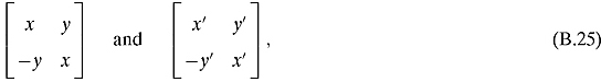
their sum is
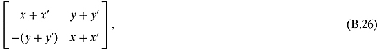
and so the set is closed under addition. Similar for scalar multiplication. This sum is also equal to
![]()
Ex. 2.2.17: A given pair 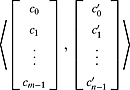 goes to
![]()
Ex. 2.2.18: An element [c0, c1; … , cm−1]T of ![]() can be seen as the element
can be seen as the element 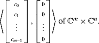
![]()
Ex. 2.3.2: The canonical basis can easily be written as a linear combination of these vectors.
Ex. 2.4.1: Both sides of Equation (2.101) are 11 and both sides of Equation (2.102) are 31.
Ex. 2.4.3: We shall show it for Equation (2.101).
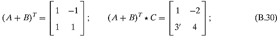
and the Trace of this matrix is 5. The right-hand side is Trace(AT * B) = −2 added to Trace(AT * C) = 7 for a sum of 5.
Ex. 2.4.5: ![]() .
.
Ex. 2.4.6: ![]() .
.
Ex. 2.4.7: ![]() .
.
![]()
![]()
![]()
![]()
Ex. 2.5.1: Their eigenvalues are –2, –2, and 4, respectively.
Ex. 2.6.1: Look at it.
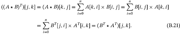
Ex. 2.6.2: The key idea is that you take the transpose of both sides of
![]()
and remember that the T operation is idempotent.
Ex. 2.6.3: The proof is the same as the hermitian case but with the dagger replaced with the transpose operation.
Ex. 2.6.4: The proof is analogous to the hermitian case.
Ex. 2.6.5: Multiply it out by its adjoint and remember the basic trigonometric identity:
![]()
Ex. 2.6.6: Multiply it by its adjoint to get the identity.
Ex. 2.6.7: If U is unitary, then U * U† = I. Similarly, if U′ is unitary, then U′ *U′† = I. Combining these we get that

![]()
Ex. 2.6.9: It is a simple observation and they are their own adjoint.
![]()
Ex. 2.7.2: No. We are looking for values such that
![]()
That would imply that za = 0 and which means either z = 0 or a = 0. If z = 0, then we would not have zb = 1 and if a = 0 we would not have xa = 5. So no such values exist.
Ex. 2.7.5: Both associations equal
Ex. 2.7.6: For ![]() and
and ![]() we have
we have
The center equality follows from these three identities that can easily be checked:
![]()
![]()
![]()
Ex. 2.7.7: They are both equal to
Ex. 2.7.8: For ![]() and
and ![]() , we have
, we have
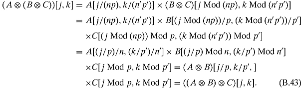
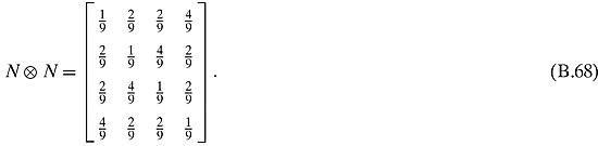
Ex. 2.7.9: For ![]() , and
, and ![]() we will have
we will have ![]() , and
, and ![]() .
.
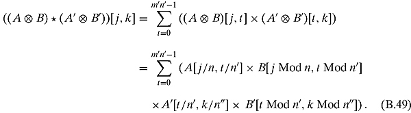
These m′n′ terms can be rearranged as follows:
CHAPTER 3
![]()
They all end up in vertex 2.
Ex. 3.1.3: The marbles in each vertex would “magically” multiply themselves and the many copies of the marbles would go to each vertex that has an edge connecting them. Think nondeterminism!
Ex. 3.1.4: The marbles would “magically” disappear.
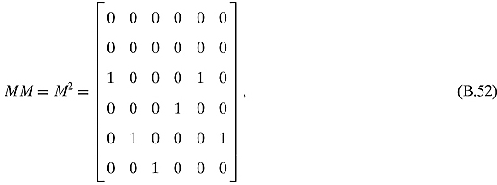
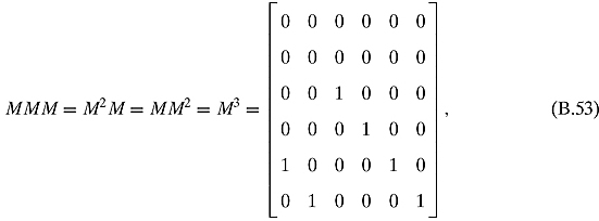
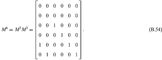
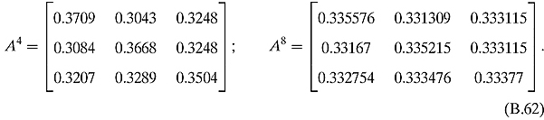
Ex. 3.1.5: The adjacency matrix is
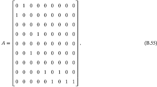
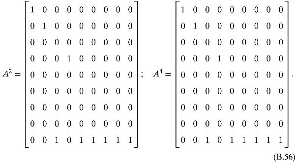
If we start in state X = [1, 1, 1, 1, 1, 1, 1, 1, 1]T, then AX = [1 1 0 1 0 1 0 2 3]T, and A2 X = A4 X = [1 1 0 1 0 0 0 0 6]T.
![]()
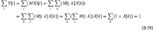
Ex. 3.2.2: We are given that ∑i M[i, k] = 1 and ∑i X[i] = 1. Then we have
Ex. 3.2.3: This is done almost exactly like Exercise 3.2.2.
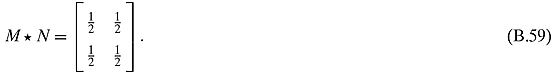
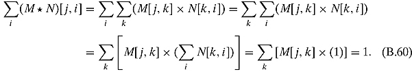
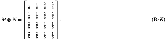
Ex. 3.2.5: Let M and N be two doubly stochastic matrices. We shall show that the jth row of M* N sums to 1 for any j. (The computation for the kth column is similar.)
Ex. 3.2.6: Let m stand for math, p stand for physics, and c stand for computer science. Then the corresponding adjacency matrix is
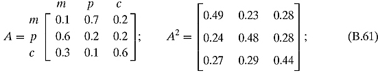
To calculate the probable majors, multiply these matrices by [1, 0, 0]T, [0, 1, 0]T, and [0, 0, 1]T.
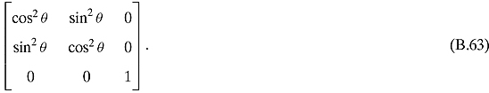
The fact that it is doubly stochastic follows from the trigonometric identity
![]()
Ex. 3.3.2: Let U be a unitary matrix. U being unitary means that
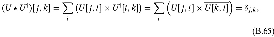
where δj,k is the Kronecker delta function. We shall show that the sum of the jth row of the modulus squared elements is 1. A similar proof shows the same for the kth column.
![]()
The first equality follows from Equation (1.49).
Ex. 3.3.3: Let U be unitary and X be a column vector such that ∑j|X[j]|2 = x.
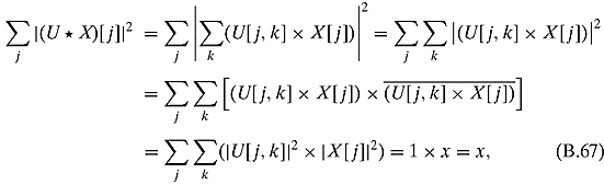
which follows from the solution to Exercise 3.3.2.
Ex. 3.4.4: For ![]() and
and ![]() , we will have
, we will have ![]() . The edge from j to k in
. The edge from j to k in ![]() will have weight
will have weight
![]()
and will correspond to the pairs of edges
![]()
Ex. 3.4.5: This is very similar to Exercise 3.4.4.
Ex. 3.4.6: “One marble traveling on the M graph and one marble traveling on the N graph” is the same as “One marble on the N graph and one marble on the M graph.”
Ex. 3.4.7: It basically means that “A marble moves from the M graph to the M′ graph and a marble moves from the N graph to the N′ graph.” It is the same as saying “Two marbles move from the M and N graph to the M′ and N′ graph, respectively. See the graph given in Equation (5.47).
CHAPTER 4
Ex. 4.1.1: The length of ![]() is
is ![]() . We get
. We get ![]() .
.
Ex. 4.1.2: This was done in the text where c = 2. The general problem is exactly the same.
Ex. 4.1.3: If they represented the same state, there would be a complex scalar c such that the second vector is the first one times c. The first component of the second vector is 2 *(1 + i), and 1 + i is the first component of the first vector. However, if we multiply the second component, we get 2 (2 − i) = 4 − 2i, not 1 − 2i. Hence, they do not represent the same state.
Ex. 4.1.9: ![]() .
.
Ex. 4.2.2: ![]() . (It flips them!) If we measure spin in state down, it will stay there; therefore, the probability to find it still in state up is zero.
. (It flips them!) If we measure spin in state down, it will stay there; therefore, the probability to find it still in state up is zero.
Ex. 4.2.3: Taking ![]() as the definition of hermitian, we consider r· A, where r is a scalar.
as the definition of hermitian, we consider r· A, where r is a scalar.
![]()
We used the fact that for any real ![]() .
.
Ex. 4.2.4: Let ![]() . M is certainly hermitian (in fact, real symmetric). Multiply it by i:
. M is certainly hermitian (in fact, real symmetric). Multiply it by i:
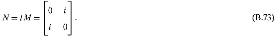
Now, N is not hermitian: the conjugate of N is ![]() , whereas every hermitian is its own conjugate.
, whereas every hermitian is its own conjugate.
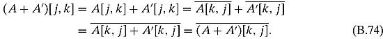
Ex. 4.2.5 Let A and A′ be two hermitian matrices.
Ex. 4.2.6 Both matrices are trivially hermitian by direct inspection (the first one has i and −i on the nondiagonal elements, and the second is diagonal with real entries). Let us calculate their products:

They do not commute.
CHAPTER 5
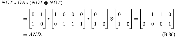
![]()
![]()
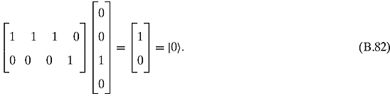
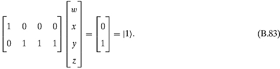
if and only if either x or y or z is 1.
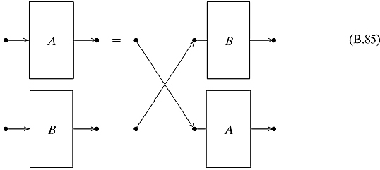
Ex. 5.2.4: It means that it does not matter which operation is the “top” and which is the “bottom,” i.e., the wires can be crossed as follows:
Ex. 5.2.5: It means that we can think of the diagram as doing parallel operations, each of which contain two sequential operations, or equivalently, we can think of the diagram as representing two sequential operations, each consisting of two parallel operations. Either way, the action of the operations are the same.
Ex. 5.3.3: Setting ![]() gives the NAND gate.
gives the NAND gate.
Ex. 5.3.4: Combining a Fredkin gate followed by a Fredkin gate gives the following:
![]()
and
![]()
Ex. 5.4.1: Except for Y all of them are their own conjugate. Simple multiplication shows that one gets the identity.
Ex. 5.4.9: One way of doing this is to show that both gates have the same matrix that performs the action.
CHAPTER 6
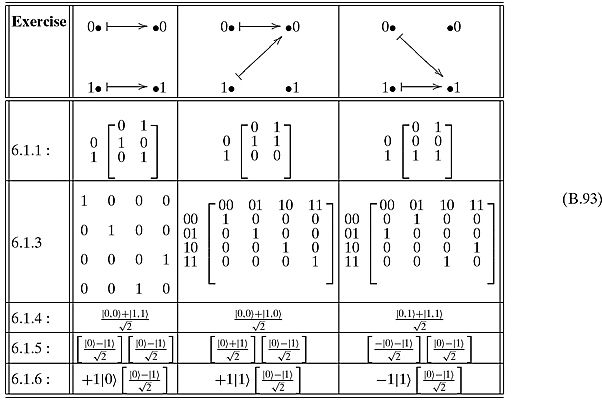
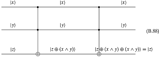
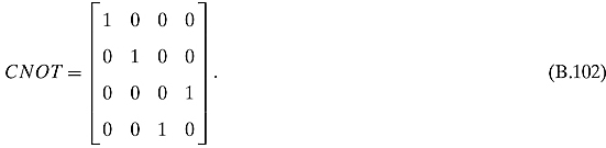
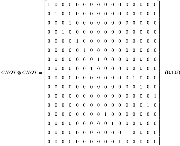
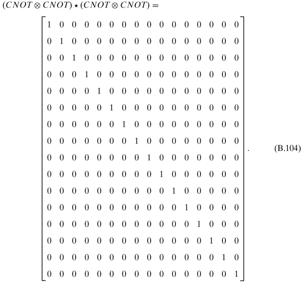
Ex 6.1.2: The conjugation of this matrix is the same as the original. If you multiply it by itself, you get I4.
Ex. 6.2.1: ![]() and 2.
and 2.
Ex. 6.2.4: We saw for n = 1, the scalar coefficient is ![]() . Assume it is true for n = k. That is the scalar coefficient of
. Assume it is true for n = k. That is the scalar coefficient of ![]() is
is ![]() . For n = k + 1, that coefficient will be multiplied by
. For n = k + 1, that coefficient will be multiplied by ![]() to get
to get
![]()
Ex. 6.2.5: It depends how far away the function is from being balanced or constant. If it is close to constant than we will probably get ![]() when we measure the top qubit. If it is close to constant, then we will probably get
when we measure the top qubit. If it is close to constant, then we will probably get ![]() . Otherwise it will be random.
. Otherwise it will be random.
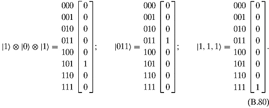
![]()
![]() ; hence, f(000) = f(011).
; hence, f(000) = f(011).
![]()
![]() ; hence, f(001) = f(010).
; hence, f(001) = f(010).
![]()
![]() ; hence, f(010) = f(001).
; hence, f(010) = f(001).
![]()
![]() ; hence, f(011) = f(000).
; hence, f(011) = f(000).
![]()
![]() ; hence, f(100) = f(111).
; hence, f(100) = f(111).
![]()
![]() ; hence, f(101) = f(110).
; hence, f(101) = f(110).
![]()
![]() ; hence, f(110) = f(101).
; hence, f(110) = f(101).
![]()
![]() ; hence, f(111) = f(101).
; hence, f(111) = f(101).
Ex. 6.4.1: For the function that "picks out" 00, we have
For the function that “picks out” 01, we have
For the function that “picks out” 11, we have
Ex. 6.4.2: The average is 36.5. The inverted numbers are 68, 35, 11, 15, 52, and 38.
Ex. 6.5.1: 654, 123, and 1.
Ex. 6.5.2: The remainders of the pairs are 1, 128, and 221.
Ex. 6.5.3: The periods are 38, 20, and 11.
Ex. 6.5.4: GCD(76 + 1, 247) = GCD(117650, 247) = 13 and GCD(76 − 1, 247) = GCD(117648, 247) = 19.13 × 19 = 247.
CHAPTER 7

Ex. 7.2.3: Observe that U can be divided into four squares: the left on top is just the 2-by-2 identity, the right on top and the left at the bottom are both the 2-by-2 zero matrix, and finally the right at the bottom is the phase shift matrix R180. Thus, ![]() , and it acts on 2 qubits, leaving the first untouched and shift the phase of the second by 180.
, and it acts on 2 qubits, leaving the first untouched and shift the phase of the second by 180.
CHAPTER 8
Ex. 8.1.2: n = 1,417,122.
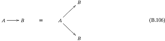
Ex. 8.1.3: The best way to show this is with a series of trees that show how to split up at each step. If at a point, the Turing machine splits into n > 2 states, then perform something like the following substitution. If n = 5, split it into four steps as follows:
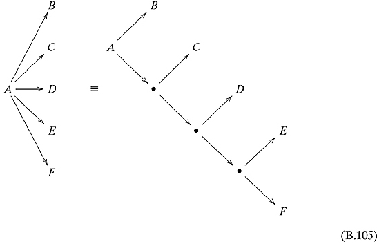
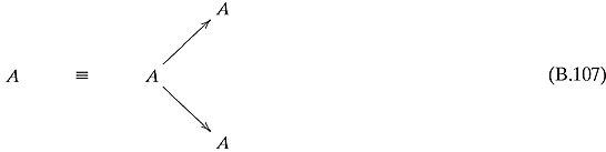
If n = 2, then no change has to be made. If n = 1, then do the following substitution:
And finally, if n = 0, make the following substitution:
Ex. 8.2.1: Following Exercise 8.1.3, every Turing machine can be made into one that at every step splits into exactly two configurations. When a real number is generated to determine which action the probabilistic Turing machine should perform, convert that real number to binary. Let that binary expansion determine which action to perform. If “0,” then go up. If “1,” then go down.
Ex 8.3.1: For a reversible Turing machine, every row of the matrix U will need to have exactly one 1 with the remaining entries 0. For a probabilistic Turing machine, every column of the matrix U will need to sum to 1.
Ex. 8.3.3: We see from the table in the text that Grover’s algorithm starts getting quicker somewhere between 10 and 15. A little analysis gives us the following table:
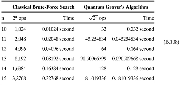
Already at n = 14, Grover’s algorithm is quicker.
CHAPTER 9
Ex 9.1.1: No. It implies that ENC(−, KE) is injective (one-to-one) and that DEC(−KD) is surjective (onto).
Ex 9.1.2: “QUANTUM CRYPTOGRAPHY IS FUN.”
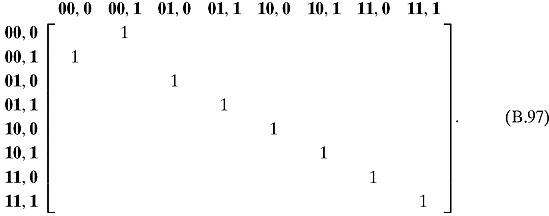
![]()
![]() with respect to + will be
with respect to + will be ![]() .
.
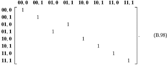
![]()
![]() with respect to + will be
with respect to + will be ![]() .
.
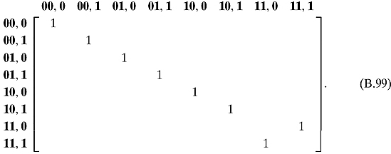
![]()
![]() with respect to + will be
with respect to + will be ![]() .
.
![]()
![]() with respect to + will be
with respect to + will be ![]() .
.
![]()
![]() with respect to X will be
with respect to X will be ![]() .
.
![]()
![]() with respect to X will be
with respect to X will be ![]() .
.
![]()
![]() with respect to X will be
with respect to X will be ![]() .
.
![]()
![]() with respect to X will be
with respect to X will be ![]() .
.
CHAPTER 10
Ex 10.1.1: All probabilities pi are positive numbers between 0 and 1. Therefore, all the logarithms log2(pi) are negative or zero, and so are all terms pi log2(pi). Their sum is negative or zero and therefore entropy is always positive (it reaches zero only if one of the probabilities is 1).
Ex 10.1.3: Choose ![]() , and P(C) = p(D) = 0. We get H(S) = 0.81128.
, and P(C) = p(D) = 0. We get H(S) = 0.81128.
Ex 10.2.1: In Equation (10.14), D is defined as the sum of the projectors ![]() weighted by their probabilities. If Alice always send one state, say
weighted by their probabilities. If Alice always send one state, say ![]() , that means that all the pi = 0, except p1 = 1. Replace them in D and you will find
, that means that all the pi = 0, except p1 = 1. Replace them in D and you will find ![]() .
.
Ex 10.2.3: Let us first write down the density operator:
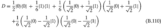
Now, let us calculate ![]() and
and ![]() :
:
![]()
Thus the matrix (we shall use the same letter D) in the standard basis is
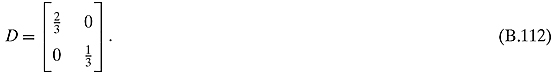
Ex 10.4.1: Suppose you send “000” (i.e., the code for “0”). What are the chances that the message gets decoded wrongly? For that to happen, at least two flips must have occurred: “110,” “011,” “101,” and “111.” Now, the first three cases occur with probability (0.25)2, and the last one with probability (0.25)3 (under the assumption that flips occur independently).
The total probability is therefore 3 * (0.25)2 + (0.25)3 = 0.20312.
Similarly when you send “111.”
CHAPTER 11
Ex 11.1.1: At first sight, the pure state
![]()
and the mixed state obtained by having ![]() or
or ![]() with equal probability seem to be undistinguishable. If you measure
with equal probability seem to be undistinguishable. If you measure ![]() in the standard basis, you will get 50% of the time
in the standard basis, you will get 50% of the time ![]() and 50% of the time
and 50% of the time ![]() . However, if you measure
. However, if you measure ![]() in the basis consisting of
in the basis consisting of ![]() ) itself, and its orthogonal
) itself, and its orthogonal
![]()
you will always detect ![]() . But, measuring the mixed state in that basis, you will get
. But, measuring the mixed state in that basis, you will get ![]() 50% of the times and
50% of the times and ![]() 50% of the times. The change of basis discriminates between the two states.
50% of the times. The change of basis discriminates between the two states.
Ex 11.1.2: Let us carry out the calculation of the average A. ![]() is, in the standard basis, of the column vector [1, eiθ]T. Thus the average is
is, in the standard basis, of the column vector [1, eiθ]T. Thus the average is
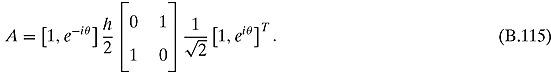
Multiplying, we get
![]()
which simplifies to
![]()
A does indeed depend on θ, and reaches a maximum at θ = 0.
Ex 11.1.3: Let us compute the tensor product of Sx with itself first (we shall ignore the factor ![]() ):
):
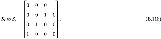
We can now calculate the average:
![]()
(using the Euler formula). We have indeed recovered the hidden phase θ!