11
Hardware
The machine does not isolate man from the great problems of nature, but plunges him more deeply into them.
Antoine de Saint Exupery, Wind, Sand, and Stars
In this chapter, we discuss a few hardware issues and proposals. Most certainly you have wondered (perhaps more than once!) whether all we have presented up to now is nothing more than elegant speculation, with no practical impact for the real world.
To bring things down to earth, we must address a very basic question: do we actually know how to build a quantum computer?
It turns out that the implementation of quantum computing machines represents a formidable challenge to the communities of engineers and applied physicists. However, there is some hope in sight: quite recently, some simple quantum devices consisting of a few qubits have been successfully built and tested. Considering the amount of resources that have been poured into this endeavor from different quarters (academia, private sector, and the military), it would not be entirely surprising if noticeable progress were made in the near future.
In Section 11.1 we spell out the hurdles that stand in the way, chiefly related to the quantum phenomenon known as decoherence. We also enumerate the wish list of desirable features for a quantum device. Sections 11.2 and 11.3 are devoted to describing two of the major proposals around: the ion trap and optical quantum computers. The last section mentions two other proposals, and lists some milestones that have been achieved so far. We conclude with some musings on the future of quantum ware.
A small disclaimer is in order. Quantum hardware is an area of research that requires, by its very nature, a deep background in quantum physics and quantum engineering, way beyond the level we have asked of our reader. The presentation will have perforce a rather elementary character. Refer to the bibliography for more advanced references.
Note to the Reader: We would have loved to assign exercises such as “build a quantum microcontroller for your robot,” or “assemble a network of quantum chips,” or something along these lines. Alas, we cannot. Nor, without violating the aforementioned disclaimer, could we ask you to carry out sophisticated calculations concerning modulations of electromagnetic fields, or similar matters. Thus, there are only few exercises scattered in this chapter (do not skip them though: your effort will be rewarded).
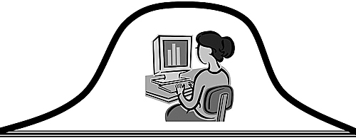
Figure 11.1. A PC that is uncoupled from the environment.
11.1 QUANTUM HARDWARE: GOALS AND CHALLENGES
In Chapter 6 we described the generic architecture of a quantum computing device: we need a number of addressable qubits, the capability of initializing them properly, applying a sequence of unitary transformation to them, and finally measuring them.
Initialization of a quantum computer is similar to initialization of a classical one: at the beginning of our computation, we set the machine in a well-defined state. It is absolutely crucial that the machine stay in the state we have put it in, till we modify it in a controlled way by means of known computational steps. For a classical computer, this is in principle quite easy to do1: a classical computer can be thought of as an isolated system. Influences from the environment can theoretically be reduced to zero. You might keep Figure 11.1 in mind.
The case of a quantum computer is rather different. As we have already seen, one of the core features of quantum mechanics is entanglement: if a system S is composed of two subsystems S1 and S2, their states may become entangled. In practice, this means that we cannot ignore what happens to S2 if we are interested in the way S1 evolves (and vice versa). Moreover, this odd phenomenon happens regardless of how physically separated the two subsystems actually are. How is this relevant to the task of building a quantum computer? The machine and its environment become entangled, preventing the evolution of the state of the quantum register from depending exclusively on which gates are applied to it. To fix our ideas, let us suppose that the quantum register in our device is a sequence of 1,000 electrons, qubits being encoded as their spin state. In this scenario, initialization means setting all the electrons to some defined spin state, as in Figure 11.2. For instance, they could be all in spin up, or all in spin down. The key point is that we need to control the global state of the register. In physics jargon, a well-defined state is known as pure state, as in Figure 11.2.

Figure 11.2. An uncoupled register initialized to spin up.
When we take our register out of isolation, these electrons tend to couple with the billions of other electrons in the environment, shifting to some superposition of spin up and spin down, as in Figure 11.3.
The problem here lies in that we have absolutely no idea about the precise initial state of the environment’s electrons, nor do we know the details of their interaction with the electrons in the quantum register. After a while, the global state of the register is no longer pure; rather, it has become a probabilistic mix of pure states, or what is known in quantum jargon as a mixed state.2 Pure states and mixed states have a different status in quantum mechanics. There is always a specific measurement that invariably returns true on a pure state. Instead, there is no such thing for mixed states, as shown by the following exercise.
Exercise 11.1.1 Consider the pure state ![]() , and the mixed state obtained1 by tossing a coin and setting it equal to
, and the mixed state obtained1 by tossing a coin and setting it equal to ![]() if the result is heads, or
if the result is heads, or ![]() if the result is tails.3 Devise an experiment that discriminates between these two states. Hint: What would happen if we measured the qubit in the following basis?
if the result is tails.3 Devise an experiment that discriminates between these two states. Hint: What would happen if we measured the qubit in the following basis?

Where precisely lies the difference between pure and mixed states?
Consider the following family of spin states:
![]()
For every choice of the angle θ, there is a distinct pure state. Each of these states is characterized by a specific relative phase, i.e., by the difference between the angles of the components of ![]() and
and ![]() in the polar representation.4 How can we physically detect their difference? A measurement in the standard basis would not do (the probabilities with respect to this basis haven’t been affected). However, a change of basis will do. Observe
in the polar representation.4 How can we physically detect their difference? A measurement in the standard basis would not do (the probabilities with respect to this basis haven’t been affected). However, a change of basis will do. Observe ![]() along the x axis, and compute the average spin value along this direction5:
along the x axis, and compute the average spin value along this direction5: ![]() . As you can verify for yourself in the next exercise, the average depends on θ!
. As you can verify for yourself in the next exercise, the average depends on θ!
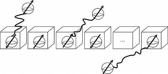
Figure 11.3. The qubits decohered as a result of coupling with the environment.
Exercise 11.1.2 Calculate ![]() . For which value of θ is the average maximum?
. For which value of θ is the average maximum?
![]()
If you now consider the mixed state of the last exercise, namely the one you get by tossing a coin and deciding for either ![]() or
or ![]() , the relative phase and its concomitant information is lost. It is precisely the lack of relative phase that separates pure states and mixed ones. One way states change from pure to mixed is through uncontrollable interaction with the environment.
, the relative phase and its concomitant information is lost. It is precisely the lack of relative phase that separates pure states and mixed ones. One way states change from pure to mixed is through uncontrollable interaction with the environment.
Definition 11.1.1 The loss of purity of the state of a quantum system as the result of entanglement with the environment is known as decoherence.
We are not going to provide a full account of decoherence6. However, it is well worth sketching how it works, as it is our formidable challenger in the path to real-life quantum computation (the Art of War states: “know thy enemy!”).
In all our descriptions of quantum systems, we have implicitly assumed that they are isolated from their environment. To be sure, they can interact with the external world. For instance, an electron can be affected by an electromagnetic field, but the interaction is, as it were, under control. The evolution of the system is described by its hamiltonian (see Section 4.3), which may include components accounting for external influences. Therefore, as long as we know the hamiltonian and the initial state, it is totally predictable. Under such circumstances, the system will always evolve from pure states to other pure states. The only unpredictable factor is measurement. Summing up: we always implictly assumed that we knew exactly how the environment affects the quantum system.
Let us now turn to a more realistic scenario: our system, say, a single electron spin, is immersed in a vast environment. Can we model this extended system? Yes, we can, by thinking of the environment as a huge quantum system, assembled out of its components.
To understand what happens, let us start small. Instead of looking at the entire environment, we shall restrict ourselves to interactions with a single external electron. Let us go back to our electron of a moment ago, and let us assume that it has become entangled with another electron to form the global state
![]()
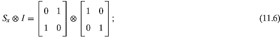
Now, let us only measure the spin of our electron in the x direction, just as we have done before. This step corresponds to the observable ![]() , i.e., the tensor of Sx with the identity on the second electron: we must therefore compute
, i.e., the tensor of Sx with the identity on the second electron: we must therefore compute
![]()
Let us do it. In matrix notation (written in the standard basis),
![]()
and (we are ignoring here the constant factor ![]() )
)
thus we are simply evaluating

The net result of our calculation is that the phase is apparently gone: there is no a trace of θ in the average value! We say this – apparently – for a reason: the phase is simply hiding behind the curtain afforded by entanglement. To “smoke the phase out,” we have to perform a measurement on both electrons. How? We simply compute the average of ![]() on
on ![]() . The value now does indeed depend on θ, as you can check in the following exercise:
. The value now does indeed depend on θ, as you can check in the following exercise:
Exercise 11.1.3 Compute ![]() .
.
![]()
It is time to wrap up what we have learned. We were able to recover the precious phase information only after measuring the second electron. Now, imagine our electron interacting with a great many peers from the environment, in an unknown manner. If we could track them all down, and measure their respective states, just like we have done above, there would be no issue. Alas, we cannot: our phase is irretrievably lost, turning our pure state into a mixed one. Note that decoherence does not cause any real collapse of the state vector. The information is still out there, marooned, as it were, in the vast quantum ocean.
Decoherence presents us with a two-pronged challenge:
![]() On the one hand, adopting basic quantum systems that are very prone to “hook up” with the environment (electrons are a very good example, as they tend to interact with other peers in their vicinity) makes it quite difficult to manage the state of our machine.
On the one hand, adopting basic quantum systems that are very prone to “hook up” with the environment (electrons are a very good example, as they tend to interact with other peers in their vicinity) makes it quite difficult to manage the state of our machine.
![]() On the other hand, we do need to interact with the quantum device after all, to initialize it, apply gates, and so on. We are part of the environment. A quantum system that tends to stay aloof (photons are the primary example) makes it difficult to access its state.
On the other hand, we do need to interact with the quantum device after all, to initialize it, apply gates, and so on. We are part of the environment. A quantum system that tends to stay aloof (photons are the primary example) makes it difficult to access its state.
How serious is the challenge afforded by decoherence? How quick are its effects? The answer varies, depending on the implementation one chooses (for instance, for single-ion qubits, as described in the next section, it is a matter of seconds). But it is serious enough to raise major concerns. You can read a leisurely account in the sprightly Scientific American article “Quantum Bug” by Graham P. Collins.
How can we even hope to build a reliable quantum computing device if decoherence is such a big part of quantum life? It sounds like a Catch-22, doesn’t it? There are, however, two main answers:
![]() A possible way out is fast gates execution: one tries to make decoherence sufficiently slow in comparison to our control, so that one has time to safely apply quantum gates first. By striving to beat Nature in the speed race, at least on very short runs, we can still hope to get meaningful results.
A possible way out is fast gates execution: one tries to make decoherence sufficiently slow in comparison to our control, so that one has time to safely apply quantum gates first. By striving to beat Nature in the speed race, at least on very short runs, we can still hope to get meaningful results.
![]() The other strategy is fault-tolerance. How can one practically achieve fault-tolerance? In Section 10.4, we have briefly sketched the topic of quantum error-correcting codes. The rationale is that using a certain redundancy, we can thwart at least some types of errors. Also, another possible strategy under the redundancy umbrella is repeating a calculation enough times, so that random errors cancel each other out.7
The other strategy is fault-tolerance. How can one practically achieve fault-tolerance? In Section 10.4, we have briefly sketched the topic of quantum error-correcting codes. The rationale is that using a certain redundancy, we can thwart at least some types of errors. Also, another possible strategy under the redundancy umbrella is repeating a calculation enough times, so that random errors cancel each other out.7
We conclude this section with an important wish list for candidate quantum computers that has been formulated by David P. DiVincenzo of IBM.
DiVincenzo’s Wish List
![]() The quantum machine must have a sufficiently large number of individually addressable qubits.
The quantum machine must have a sufficiently large number of individually addressable qubits.
![]() It must be possible to initialize all the qubits to the zero state, i.e.,
It must be possible to initialize all the qubits to the zero state, i.e., ![]() .
.
![]() The error rate in doing computations should be reasonably low, i.e., decoherence time must be substantially longer than gate operation time.
The error rate in doing computations should be reasonably low, i.e., decoherence time must be substantially longer than gate operation time.
![]() We should be able to perform elementary logical operations between pairs of qubits.
We should be able to perform elementary logical operations between pairs of qubits.
![]() Finally, we should be able to reliably read out the results of measurements.
Finally, we should be able to reliably read out the results of measurements.
These five points spell out the challenge that every prospective implementation of a quantum computing device must meet. We are now going to see a few of the proposals that have emerged in the last ten odd years.
11.2 IMPLEMENTING A QUANTUM COMPUTER I: ION TRAPS
Before we start discussing concrete implementations, let us remind ourselves that a qubit is a state vector in a two-dimensional Hilbert space. Therefore, any physical quantum system whose state space has dimension 2N can, at least in principle, be used to store an addressable sequence of N qubits (a q-register, in the notation of Chapter 7).
What are the options?
Generally, the standard strategy is to look for quantum systems with a two-dimensional state space. One can then implement q-registers by assembling a number of copies of such systems. The canonical two-dimensional quantum systems are particles with spin. Electrons, as well as single atoms, have spin. There is thus plenty of room in nature for encoding qubits. Spin is not the only one: another natural choice is excited states of atoms, as we are going to see in a moment.
Let us first sumnmarize all the steps we need:
![]() Initialize all particles to some well-defined state.
Initialize all particles to some well-defined state.
![]() Perform controlled qubit rotations on a single particle (this step will implement a single-qubit gate).
Perform controlled qubit rotations on a single particle (this step will implement a single-qubit gate).
![]() Be able to mix the states of two particles (this step aims at implementing a universal two-qubit gate).
Be able to mix the states of two particles (this step aims at implementing a universal two-qubit gate).
![]() Measure the state of each individual particle.
Measure the state of each individual particle.
![]() Keep the system of particles making up our q-register as insulated as possible from the environment, at least for the short period of time when quantum gates are applied.
Keep the system of particles making up our q-register as insulated as possible from the environment, at least for the short period of time when quantum gates are applied.
The first proposal for quantum hardware is known as the ion trap. It is the oldest one, going back to the mid-nineties, and it is still the most popular candidate for quantum hardware.8
The core idea is simple: as you may recall from your chemistry classes, an ion is an electrically charged atom. Ions can be of two types: they are either positive ion, or cations, having lost one or more electrons. Or they are negative ions, or anions, having acquired some electrons. Ionized atoms can be acted upon by means of an electromagnetic field, as they are electrically charged; more precisely, we can confine our ionized atom in a specific volume, known as ion trap (Figure 11.4).

Figure 11.4. An ion in a trap.
In practice, experiments have been conducted with positive ions of calcium: Ca+. First, the metal is brought to its gaseous state. Next, the single atoms are stripped of some of their electrons, and third, by means of a suitable electromagnetic field, the resulting ions are confined to the trap.
How are qubits encoded? An atom can be in a excited state or in a ground state (Figure 11.5).
These two states represent two energy levels of the atom and they form an orthogonal basis for a two-dimensional Hilbert space. As we have seen in Chapter 4 (photoelectric effect), if we pump energy into an atom that is in ground state by making it absorb a photon, it will raise to its excited state. Conversely, the atom can lose its energy by emitting a photon. This process is known as optical pumping and it is performed using a laser, i.e., a coherent beam of light. The reason for using a laser is that it has an extremely high resolution, allowing the operator to “hit” single ions and thereby achieving a good control of the quantum register. Through optical pumping we can initialize our register to some initial state with a high degree of fidelity (almost 100%).
Next, we need to manipulate the register. As we mentioned in Section 7.2, there is a considerable degree of freedom in quantum computing when it comes to which particular set of gates is implemented, as long as the set is complete. The particular choice depends on the hardware architecture: one chooses gates that are easy to implement and provide a good degree of fidelity. In the ion trap model, the usual choice is as follows:
![]() Single-qubit rotation: By “hitting” the single ion with a laser pulse of a given amplitude, frequency, and duration, one can rotate its state appropriately.
Single-qubit rotation: By “hitting” the single ion with a laser pulse of a given amplitude, frequency, and duration, one can rotate its state appropriately.
![]() Two-qubit gates: The ions in the trap are, in a sense, strung together by what is known as their common vibrational modes. Again, using a laser one can affect their common mode, achieving the desired entanglement (see the paper by Holzscheiter for details). The original choice for a two-qubit gate was the controlled-NOT gate, which was proposed in 1995 by Cirac and Zoller (1995). Recently, several other more reliable schemes have been implemented.
Two-qubit gates: The ions in the trap are, in a sense, strung together by what is known as their common vibrational modes. Again, using a laser one can affect their common mode, achieving the desired entanglement (see the paper by Holzscheiter for details). The original choice for a two-qubit gate was the controlled-NOT gate, which was proposed in 1995 by Cirac and Zoller (1995). Recently, several other more reliable schemes have been implemented.
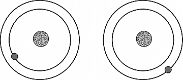
Figure 11.5. Ground and excited states.
The last step is measurement. Essentially, the same mechanism we use for setting the qubits can be employed for readouts. How? Aside from the two main long-lived states![]() and
and ![]() (ground and excited), the ion can enter a short-lived state, let us call it
(ground and excited), the ion can enter a short-lived state, let us call it ![]() (“s” is for short), when gently hit by a pulse. Think of
(“s” is for short), when gently hit by a pulse. Think of ![]() as sitting in the middle between the other two. If the ion is in the ground state and gets pushed to
as sitting in the middle between the other two. If the ion is in the ground state and gets pushed to ![]() it will revert to ground and emit a photon. On the other hand, if it is in an the excited state, it will not. By repeating the transition many times, we can detect the photons emitted (if any) and thus establish where the qubit is.
it will revert to ground and emit a photon. On the other hand, if it is in an the excited state, it will not. By repeating the transition many times, we can detect the photons emitted (if any) and thus establish where the qubit is.
To conclude this section, let us list the main strengths and weaknesses of the ion trap model:
![]() On the plus side, this mode has long coherence time, in the order of 1–10 seconds. Secondly, the measurements are quite reliable, very close to 100%. Finally, one can transport qubits around in the computer, which is a nice feature to have (remember, no copying allowed, so moving things around is good).
On the plus side, this mode has long coherence time, in the order of 1–10 seconds. Secondly, the measurements are quite reliable, very close to 100%. Finally, one can transport qubits around in the computer, which is a nice feature to have (remember, no copying allowed, so moving things around is good).
![]() On the minus side, the ion trap is slow, in terms of gate time (slow here means that it takes tens of milliseconds). Secondly, it is not apparent how to scale the optical part to thousands of qubits.
On the minus side, the ion trap is slow, in terms of gate time (slow here means that it takes tens of milliseconds). Secondly, it is not apparent how to scale the optical part to thousands of qubits.
11.3 IMPLEMENTING A QUANTUM COMPUTER II: LINEAR OPTICS
The second implementation of a quantum machine we are going to consider is linear optics. Here, one builds a quantum machine out of sheer light!
To build a quantum computer, the very first step is to clearly state how we are going to implement qubits. Now, as we said in Section 5.1, every quantum system that has dimension 2 is, in principle, a valid candidate. Quanta of light, alias photons, are good enough, thanks to the physical phenomenon known as polarization (see Section 4.3). We have all seen polarization at work: a beam of light passes through a polarization filter, and the result is a coherent beam of light, i.e., an electromagnetic wave that vibrates along a specific plane.
As photon can be polarized, one can stipulate how qubits are implemented: a certain polarization axis, say vertical polarization, will model|0, whereas|1will be represented by horizontal polarization.
So much for qubits. Initialization here is straightforward: a suitable polarization filter will do. Gates are less trivial, particularly entanglement gates, as photons have a tendency to stay aloof. It therefore pays to be on the economical side, i.e., to implement some small universal set of quantum gates. We have met the controlled-NOT gate in Chapter 5. If one were to follow the simple-minded route, controlled-NOT would require a two-photon interaction. This happens very seldom, and makes this venue quite impractical. But, as it often happens, there is a way around.
To create controlled-NOT, we need control and target inputs and we need more optical tools. Specifically, we need mirrors, polarizing beam splitters, additional ancillary photons, and single-photon detectors. This approach is known as linear optics quantum computing, or LOQC, as it uses only linear optics principles and methodologies. In LOQC, the nonlinearity of measurements arises from the detection of additional, ancillary photons. Figure 11.6 is a schematic picture of a LOQC controlled-NOT gate (details can be found in Pittman, Jacobs, and Franson (2004).

Figure 11.6. Basic idea of LOQC-based controlled-NOT gate.
Measurement of the final output presents no difficulties. A combination of polarization filters and single-photon detectors will do.
Before we quit this section let us point out strengths and weaknesses of the optical scheme:
![]() On the plus side, light travels. This means that quantum gates and quantum memory devices can be easily connected via optical fibers. In other approaches, like the ion trap, this step can be a quite complex process. This plus is indeed a big one, as it creates a great milieu for distributed quantum computing.
On the plus side, light travels. This means that quantum gates and quantum memory devices can be easily connected via optical fibers. In other approaches, like the ion trap, this step can be a quite complex process. This plus is indeed a big one, as it creates a great milieu for distributed quantum computing.
![]() On the minus side, unlike electrons and other matter particles, it is not easy for photons to become entangled. This is actually a plus, as it prevents entanglement with its environment (decoherence), but it also makes gate creation a bit more challenging.
On the minus side, unlike electrons and other matter particles, it is not easy for photons to become entangled. This is actually a plus, as it prevents entanglement with its environment (decoherence), but it also makes gate creation a bit more challenging.
11.4 IMPLEMENTING A QUANTUM COMPUTER III: NMR AND SUPERCONDUCTORS
Aside the two models described in the last sections, there are currently several other proposals under investigation, and more may emerge soon. We mention in passing two others that have received a lot of attention in the last years.
Nuclear Magnetic Resonance (NMR). The idea here is to encode qubits not as single particles or atoms, but as global spin states of many molecules in some fluid. These molecules float in a cup, which is placed in an NMR machine, quite akin to the devices used in hospitals for magnetic resonance imaging. This large ensemble of molecules has plenty of built-in redundancy, which allows it to maintain coherence for a relatively long time span (several seconds).
The first two-qubit NMR computers were demonstrated in 1998 by J.A. Jones and M. Mosca at Oxford University and at the same time by Isaac L. Chuang at IBM’s Almaden Research Center, together with coworkers at Stanford University and MIT. Berggren quoted in the references.
Superconductor Quantum Computers (SQP). Whereas NMR uses fluids, SQP employs superconductors.9 How? By means of Josephson junctions – thin layers of nonconducting material sandwiched between two pieces of superconducting metal. At very low temperatures, electrons within a superconductor become, as they were, friends, and pair up to form a “superfluid” flowing with no resistance and traveling through the medium as a single, uniform wave pattern. This wave leaks into the insulating middle. The current flows back and forth through the junction much like a ping-pong ball, in a rhythmic fashion.
How are qubits implemented? Through what is now known as the Josephson junction qubit. In this implementation, the ![]() and
and ![]() states are represented by the two lowest-frequency oscillations of the currents flowing back and forth through the junction. The frequency of these oscillations is very high, being of the order of billions of times per second.
states are represented by the two lowest-frequency oscillations of the currents flowing back and forth through the junction. The frequency of these oscillations is very high, being of the order of billions of times per second.
Where are we now?
In 2001 the first execution of Shor’s algorithm was carried out at IBM’s Almaden Research Center and Stanford University. They factored the number 15: not an impressive number by any means, but a definite start! (By the way, the answer was 15 = 5 * 3.)
In 2005, using NMR, a 12-qubit quantum register was benchmarked. So far at least, scalability seems to be a major hurdle. Progress has been made almost a qubit at a time, in the last few years. On the positive side, new proposals and methodologies crop up in a continuous stream.
If you wish to know more about recent news in quantum hardware research, probably the best course is to take a look at the NIST Road Map. NIST, the US National Institute of Science and Technology, a major force in the ongoing effort to implement quantum computing machines, has recently released a comprehensive road map listing all major directions toward quantum hardware, as well as comparison tables pointing at weaknesses and strengths of each individual approach. You can download it at NIST Web site: http://qist.lanl.gov/qcomp_map.shtml.
As you can imagine from this brief survey, people are pretty busy at the moment, trying to make the magic quantum work.
It is worth mentioning that as of the time of this writing (late 2007), there are already three companies whose main business is developing quantum computing technologies: D-Wave Systems, MagicQ, and Id Quantique. Recently (February 13, 2007), D-Wave has publicly demonstrated a prototypical quantum computer, known as Orion, at the Historical Museum in Mountain View, CA. Orion was apparently able to play the popular Sudoku game. D-Wave’s announcement has generated some expected and healthy skepticism among academic researchers.
11.5 FUTURE OF QUANTUM WARE
At last, the future. The great physicist Niels Bohr, a major protagonist in the development of quantum mechanics, had a great punch line: “Prediction is always hard, especially of the future.”10
We could not agree more. What we think is safe to say is that there is a reasonable likelihood that quantum computing may become a reality in the future, perhaps even in the relatively near future. If that happens, it is also quite likely that many areas of information technology will be affected. Certainly, the first thought goes to communication and cryptography. These areas are noticeably ahead, in that some concrete quantum encryption systems have been implemented and tested.
Assuming that sizeable quantum devices will be available at some point in time, there is yet another important area of computer science where one can reasonably expect some impact of quantum computation, namely, artificial intelligence. It has been suggested in some quarters that the phenomenon of consciousness has some links with the quantum (see, for instance, the tantalizing paper by Paola Zizzi or either of these two books by Sir Roger Penrose, 1994, 1999). Some people even go as far as saying that our brain may be better modeled as an immense quantum computing network than are traditional neural networks (although this opinion is not shared by most contemporary neuroscientists and cognitive scientists). Be that as it may, a new area of research has already been spawned that merges traditional artificial intelligence with quantum computing. The interaction happens both ways: for instance, artificial intelligence methodologies such as genetic algorithms have been proposed as a way to design quantum algorithms. Essentially, genes encode candidate circuits and selection and mutation do the rest. This is an important direction, as for now our understanding of quantum algorithm design is still rather limited. On the other hand, quantum computing suggests new tools for artificial intelligence. A typical example is quantum neural networks. Here, the idea is to replace activation maps with complex valued ones, akin to what we have seen in Section 3.3.
Beyond these relatively tame predictions, there is the vast expanse of science fiction out there. Interestingly, quantum computing has already percolated into science fiction (the nextQuant blog maintains a current list of science fiction works with quantum computing themes). For instance, the well-known science fiction writer Greg Egan has written a new book called Schild’s Ladder (Egan, 2002), in which he speculates about the role of quantum computing devices in the far future to enhance mind capabilities. True? False?
All too often, the dreams of today are the reality of tomorrow.
References: Literature in the topics covered by this chapter abounds, although it is a bit difficult for nonexperts to keep track of it. Here are just a few useful pointers:
For decoherence, Wojciech H. Zurek has an excellent readable paper: Zurek (2003).
David P. DiVincenzo’s rules can be found in DiVincenzo.
The ion trap model is discussed in a number of places. A good general reference is the paper by M. Holzscheiter.
Optical computers are clearly and elegantly presented in a paper by Pittman, Jacobs, and Franson (2004).
For NMR computing, see Vandersypen et al. (2001).
An article by Karl Berggren (2004) provides a good introduction to superconductor quantum computing.
1 In reality, of course, classical machines are also prone to errors.
2 The density matrix, which we introduced in Section 10.2 in order to talk about entropy, is also the fundamental tool for studying mixed states. Indeed, a single pure quantum state ![]() is associated with the special form of the density operator
is associated with the special form of the density operator ![]() , whereas an arbitrary mixed state can be represented by a generic density operator.
, whereas an arbitrary mixed state can be represented by a generic density operator.
3 For the readers of Section 10.2: the mixed state is represented by the density matrix ![]() .
.
4 It is only this relative phase that has some physical impact, as we are going to see in a minute. Indeed, multiplying both components by exp(iθ) would simply rotate them by the same angle and generate an entirely equivalent physical state, as we pointed out in Section 4.1.
5 The formula for the average as well as the hermitian Sx were described in Section 4.2.
6 Decoherence has been known since the early days of quantum mechanics. However, in recent times it has received a great deal of attention, not only in relation to quantum computing, but as a formidable tool for understanding how our familiar classical world emerges out of the uncanny quantum world. How come we do not normally see interference when dealing with macroscopic objects? An answer is provided by decoherence: large objects tend to decohere very fast, thereby losing their quantum features. An intriguing survey of decoherence as a way of accounting for classical behavior of macroscopic objects is Zurek (2003).
7 Caveat: one cannot repeat too many times, else the benefits of quantum parallelism will get totally eroded!
8 The first quantum gate, the controlled-NOT, was experimentally realized with trapped ions by C. Monroe and D. Wineland in 1995. They followed a proposal by Cirac and Zoller put forward a year earlier.
9 A superconductor is matter at very low temperature, exhibiting so-called superconductivity properties.
10 The same line is sometimes attributed to Yogi Berra.