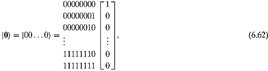
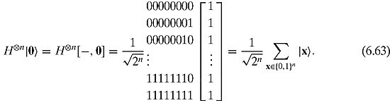
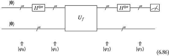
6

Algorithms

---

 

 

 

 

Computer Science is no more about computers than astronomy is about telescopes.

E.W. Dijkstra

Algorithms are often developed long before the machines they are supposed to run on. Classical algorithms predate classical computers by millennia, and similarly, there exist several quantum algorithms before any large-scale quantum computers have seen the light of day. These algorithms manipulate qubits to solve problems and, in general, they solve these tasks more efficiently than classical computers.

Rather than describing the quantum algorithms in the chronological order in which they were discovered, we choose to present them in order of increasing difficulty. The core ideas of each algorithm are based on previous ones. We start at tutorial pace, introducing new concepts in a thorough way. Section 6.1 describes Deutsch’s algorithm that determines a property of functions from{0, 1} to {0, 1}. In Section 6.2 we generalize this algorithm to the Deutsch–Jozsa algorithm, which deals with a similar property for functions from{0, 1}ⁿ to{0, 1}. Simon’s periodicity algorithm is described in Section 6.3. Here we determine patterns of a function from{0, 1}ⁿ to {0, 1}ⁿ. Section 6.4 goes through Grover’s search algorithm that can search an unordered array of size n in time as opposed to the usual n time. The chapter builds up to the ground-breaking Shor’s factoring algorithm done in Section 6.5. This quantum algorithm can factor numbers in polynomial time. There are no known classical algorithms that can perform this feat in such time.

 

---

Reader Tip. This chapter may be a bit overwhelming on the first reading. After reading Section 6.1, the reader can move on to Section 6.2 or Section 6.4. Shor’s algorithm can safely be read after Section 6.2.

---

 

6.1 DEUTSCH’S ALGORITHM

All quantum algorithms work with the following basic framework:

The system will start with the qubits in a particular classical state.

From there the system is put into a superposition of many states.

This is followed by acting on this superposition with several unitary operations.

And finally, a measurement of the qubits.

Of course, there will be several variations of this theme. Nevertheless, it will be helpful to keep this general scheme in mind as we proceed.

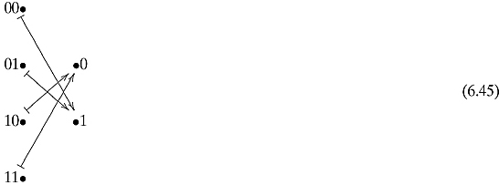
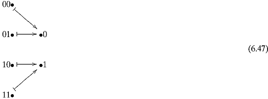
The simplest quantum algorithm is Deutsch’s algorithm, which is a nice algorithm that solves a slightly contrived problem. This algorithm is concerned with functions from the set {0, 1} to the set {0, 1}. There are four such functions that might be visualized as

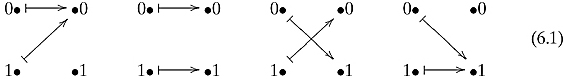
Call a function f : {0, 1} → {0, 1} balanced if f (0) ≠ f (1), i.e., it is one to one. In contrast, call a function constant if f (0) = f (1). Of the four functions, two are balanced and two are constant.

Deutsch’s algorithm solves the following problem: Given a function f : {0, 1} → {0, 1} as a black box, where one can evaluate an input, but cannot “look inside” and “see” how the function is defined, determine if the function is balanced or constant.

With a classical computer, one would have to first evaluate f on one input, then evaluate f on the second input, and finally, compare the outputs. The following decision tree shows what a classical computer must do:

The point is that with a classical computer, f must be evaluated twice. Can we do better with a quantum computer?

A quantum computer can be in a superposition of two basic states at the same time. We shall use this superposition of states to evaluate both inputs at one time.

In classical computing, evaluating a given function f corresponds to performing the following operation:

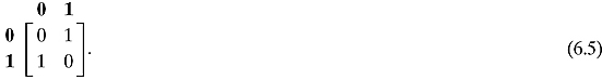
As we discussed in Chapter 5, such a function can be thought of as a matrix acting on the input. For instance, the function

is equivalent to the matrix

Multiplying state on the right of this matrix would result in state , and multiplying state on the right of this matrix would result in state . The column name is to be thought of as the input and the row name as the output.

Exercise 6.1.1 Describe the matrices for the other three functions from {0, 1} to {0, 1}.

However, this will not be enough for a quantum system. Such a system demands a little something extra: every gate must be unitary (and thus reversible). Given the output, we must be able to find the input. If f is the name of the function, then the following black-box U_f will be the quantum gate that we shall employ to evaluate input:

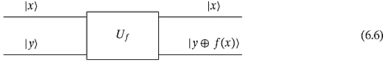
The top input, , will be the qubit value that one wishes to evaluate and the bottom input, , controls the output. The top output will be the same as the input qubit and the bottom output will be the qubit , where is XOR, the exclusive-or operation (binary addition modulo 2.) We are going to write from left to right the top qubit first and then the bottom. So we say that this function takes the state to the state . If y = 0, this simplifies to . This gate can be seen to be reversible as we may demonstrate by simply looking at the following circuit:

State goes to , which further goes to

where the first equality is due to the associativity of and the second equality holds because is idempotent. From this we see that U_f is its own inverse.

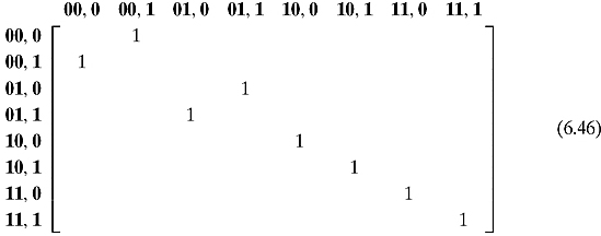
In quantum systems, evaluating f is equivalent to multiplying a state by the unitary matrix U_f. For function (6.4), the corresponding unitary matrix, U_f ,is

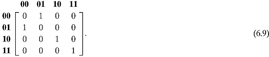
Remember that the top column name corresponds to the input and the left-hand row name corresponds to the outputs . A 1 in the xy column and the x′y′ row means that for input , the output will be .

Exercise 6.1.2 What is the adjoint of the matrix given in Equation (6.9)? Show that this matrix is its own inverse.

Exercise 6.1.3 Give the unitary matrices that correspond to the other three functions from {0, 1} to {0, 1}. Show that each of the matrices is its own adjoint and hence all are reversible and unitary.

Let us remind ourselves of the task at hand. We are given such a matrix that expresses a function but we cannot “look inside” the matrix to “see” how it is defined. We are asked to determine if the function is balanced or constant.

Let us take a first stab at a quantum algorithm to solve this problem. Rather than evaluating f twice, we shall try our trick of superposition of states. Instead of having the top input to be either in state or in state , we shall put the top input in state

which is “half-way” and “half-way” . The Hadamard matrix can place a qubit in such a state.

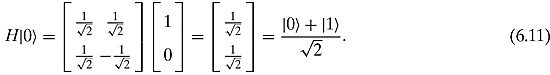
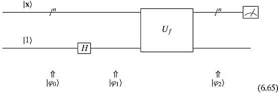
The obvious (but not necessarily correct) state to put the bottom input into is state . Thus we have the following quantum circuit:

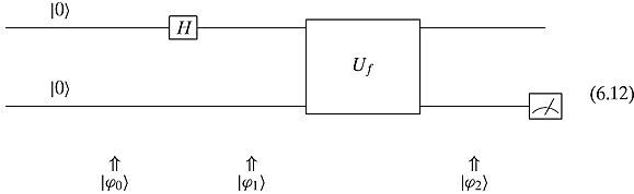
The at the bottom of the quantum circuit will be used to describe the state of the qubits at each time click.

In terms of matrices this circuit corresponds to

The tensor product can be written as

and the entire circuit is then

We shall carefully examine the states of the system at every time click. The system starts in

We then apply the Hadamard matrix only to the top input − leaving the bottom input alone − to get

After multiplying with U_f, we have

For function (6.4), the state would be

Exercise 6.1.4 Using the matrices calculated in Exercise 6.1.3, determine the state for the other three functions.

If we measure the top qubit, there will be a 50–50 chance of finding it in state and a 50–50 chance of finding it in state . Similarly, there is no real information to be gotten by measuring the bottom qubit. So the obvious algorithm does not work. We need a better trick.

Let us take another stab at solving our problem. Rather than leaving the bottom qubit in state , let us put it in the superposition state:

Notice the minus sign. Even though there is a negation, this state is also “half-way” in state and “half-way” in state . This change of phase will help us get our desired results. We can get to this superposition of states by multiplying state with the Hadamard matrix. We shall leave the top qubit as an ambiguous .

In terms of matrices, this becomes

Let us look carefully at how the states of the qubits change.

After the Hadamard matrix, we have

Applying U_f, we get

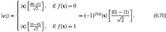
where means the opposite of f(x). Therefore, we have

Remembering that a− b = (−1)(b− a), we might write this as

What would happen if we evaluate either the top or the bottom state? Again, this does not really help us. We do not gain any information if we measure the top qubit or the bottom qubit. The top qubit will be in state and the bottom qubit will be either in state or in state . We need something more.

Now let us combine both these attempts to actually give Deutsch’s algorithm.

Deutsch’s algorithm works by putting both the top and the bottom qubits into a superposition. We will also put the results of the top qubit through a Hadamard matrix.

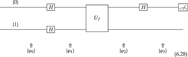
In terms of matrices this becomes

or

At each point of the algorithm the states are as follows:

We saw from our last attempt at solving this problem that when we put the bottom qubit into a superposition and then multiply by U_f, we will be in the superposition

Now, with in a superposition, we have

For example, if f(0) = 1 and f(1) = 0, the topqubit becomes

Exercise 6.1.5 For each of the other three functions from the set {0, 1} to the set {0, 1}, describe what would be.

For a general function f, let us look carefully at

If f is constant, this becomes either

(depending on being constantly 0 or constantly 1).

If f is balanced, it becomes either

(depending on which way it is balanced).

Summing up, we have that

Remembering that the Hadamard matrix is its own inverse that takes to and takes to , we apply the Hadamard matrix to the top qubit to get

For example, if f(0) = 1 and f (1) = 0, then we get

Exercise 6.1.6 For each of the other three functions from the set {0, 1} to the set {0, 1}, calculate the value of .

Now, we simply measure the top qubit. If it is in state , then we know that f is a constant function, otherwise it is a balanced function. This was all accomplished with only one function evaluation as opposed to the two evaluations that the classical algorithm demands.

Notice that although the ±1 tells us even more information, namely, which of the two balanced functions or two constant functions we have, measurement will not grant us this information. Upon measuring, if the function is balanced, we will measure regardless if the state was or .

The reader might be bothered by the fact that the output of the top qubit of U_f should not change from being the same as the input. However, the inclusion of the Hadamard matrices changes things around, as we saw in Section 5.3. This is the essence of the fact that the top and the bottom qubits are entangled.

Did we perform a magic trick here? Did we gain information that was not there? Not really. There are four possible functions, and we saw in decision tree (6.2) that with a classical computer we needed two bits of information to determine which of the four functions we were given. What we are really doing here is changing around the information. We might determine which of the four functions is the case by asking the following two questions: “Is the function balanced or constant?” and “What is the value of the function on 0?” The answers to these two questions uniquely describe each of the four functions, as described by the following decision tree:

The Hadamard matrices are changing the question that we are asking (change of basis). The intuition behind the Deutsch algorithm is that we are really just performing a change of basis problem as discussed at the end of Section 2.3. We might rewrite quantum circuit (6.28) as

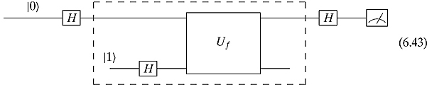
We start in the canonical basis. The first Hadamard matrix is used as a change of basis matrix to go into a balanced superposition of basic states. While in this noncanonical basis, we evaluate f with the bottom qubit in a superposition. The last Hadamard matrix is used as a change of basis matrix to revert back to the canonical basis.

6.2 THE DEUTSCH–JOZSA ALGORITHM

Let us generalize the Deutsch algorithm to other functions. Rather than talking about functions f : {0, 1} → {0, 1}, let us talk about functions with a larger domain. Consider functions f : {0, 1}ⁿ → {0, 1}, which accept a string of n 0’s and 1’s and outputs a zero or one. The domain might be thought of as any natural number from 0to2ⁿ − 1.

We shall call a function f : {0, 1}ⁿ → {0, 1} balanced if exactly half of the inputs go to 0 (and the other half go to 1). Call a function constant if all the inputs go to 0 or all the inputs go to 1.

Exercise 6.2.1 How many functions are there from {0, 1}ⁿ to {0, 1}? How many of them are balanced? How many of them are constant?

The Deutsch–Jozsa algorithm solves the following problem: Suppose you are given a function from {0, 1}ⁿ to {0, 1} which you can evaluate but cannot “see” the way it is defined. Suppose further that you are assured that the function is either balanced or constant. Determine if the function is balanced or constant. Notice that when n = 1, this is exactly the problem that the Deutsch algorithm solved.

Classically, this algorithm can be solved by evaluating the function on different inputs. The best case scenario is when the first two different inputs have different outputs, which assures us that the function is balanced. In contrast, to be sure that the function is constant, one must evaluate the function on more than half the possible inputs. So the worst case scenario requires function evaluations. Can we do better?

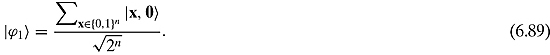
In the last section, we solved the problem by entering into a superposition of two possible input states. In this section, we solve the problem by entering a superposition of all 2ⁿ possible input states.

The function f will be given as a unitary matrix that we shall depict as

with n qubits (denoted as ) as the top input and output. For the rest of this chapter, a binary string is denoted by a boldface letter. So we write the top input as . The bottom entering control qubit is . The top output is which will not be changed by U_f. The bottom output of U_f is the single qubit . Remember that although x is n bits, f(x) is one bit and hence we can use the binary operation . It is not hard to see that U_f is its own inverse.

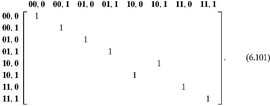
Example 6.2.1 Consider the following balanced function from {0, 1}² to {0, 1}:

This function shall be represented by the following 8-by-8 unitary matrix:

(the zeros are omitted for readability).

Exercise 6.2.2 Consider the balanced function from {0, 1}² to {0, 1}:

Give the corresponding 8-by-8 unitary matrix.

Exercise 6.2.3 Consider the function from {0, 1}² to {0, 1} that always outputs a 1. Give the corresponding 8-by-8 unitary matrix.

In order to place a single qubit in a superposition of and , we used a single Hadamard matrix. To place n qubits in a superposition, we are going to use the tensor product of n Hadamard matrices. What does such a tensor product look like? It will be helpful to do some warm-up exercises. Let us calculate H, which we may write as , and ; and look for a pattern. Our goal will be to find a pattern for .

Remember that the Hadamard matrix is defined as

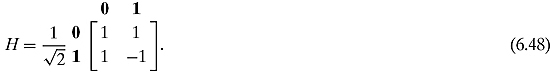
Notice that , where i and j are the row and column numbers in binary and ^ is the AND operation. We might then write the Hadamard matrix as

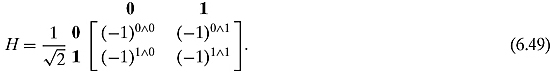
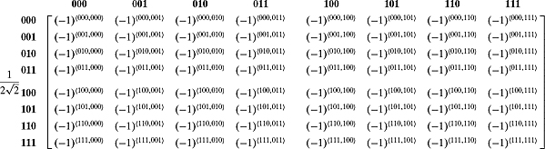
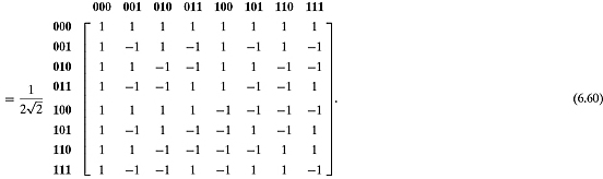
Notice that we are thinking of 0 and 1 as both Boolean values and numbers that are exponents. (Remember: (−1)⁰ = 1 and (−1)¹ = −1.) With this trick in mind we can then calculate

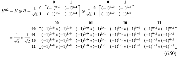
When we multiply (−1)^x by (−1)^y, we are not interested in (−1)^x+y. Rather, we are interested in the parity of x and y. So we shall not add x and y but take their exclusive-or . This leaves us with

Exercise 6.2.4 Prove by induction that the scalar coefficient of is

Thus, we have reduced the problem to determining if the exponent of (−1) is odd or even. The only time that this exponent should change is when the (−1) is in the lower-right-hand corner of a matrix. When we calculate we will again multiply each entry of by the appropriate element of H. If we are in the lower-right-hand corner, i.e., the (1, 1) position, then we should toggle the exponent of (−1).

The following operation will be helpful. We define

as follows: Given two binary strings of length n, x =x₀x₁x₂… x_n−1 and y =y₀y₁y₂… y_n−1,we say

Basically, this gives the parity of the number of times that both bits are at 1.¹

If x and y are binary strings of length n, then is the pointwise (bitwise) exclusive-or operation, i.e.,

The function satisfies the following properties:

(i)

(ii)

With this notation, it is easy to write as

From this, we can write a general formula for as

where i and j are the row and column numbers in binary.

What happens if we multiply a state with this matrix? Notice that all the elements of the leftmost column of are +1. So if we multiply with the state

we see that this will equal the leftmost column of :

For an arbitrary basic state , which can be represented by a column vector with a single 1 in position y and 0’s everywhere else, we will be extracting the y th column of :

Let us return to the problem at hand. We are trying to tell whether the given function is balanced or constant. In the last section, we were successful by placing the bottom control qubit in a superposition. Let us see what would happen if we did the same thing here.

In terms of matrices this amounts to

For an arbitrary x = x₀x₁x₂ … x_n−1 as an input in the top n qubits, we will have the following states:

After the bottom Hadamard matrix, we have

Applying U_f we get

where means the opposite of f (x).

This is almost exactly like Equation (6.27) in the last section. Unfortunately, it is just as unhelpful.

Let us take another stab at the problem and present the Deutsch–Jozsa algorithm. This time, we shall put into a superposition in which all 2ⁿ possible strings have equal probability. We saw that we can get such a superposition by multiplying by . Thus, we have

In terms of matrices this amounts to

Each state can be written as

(as in Equation (6.63)). After applying the U_f unitary matrix, we have

Finally, we apply to the top qubits that are already in a superposition of different x states to get a superposition of a superposition

from Equation (6.64). We can combine parts and “add” exponents to get

Now the top qubits of state are measured. Rather than figuring out what we will get after measuring the top qubit, let us ask the following question: What is the probability that the top qubits of will collapse to the state ? We can answer this by setting z = 0 and realizing that for all x. In this case, we have reduced to

So, the probability of collapsing to is totally dependent on f(x). If f(x) is constant at 1, the top qubits become

If f(x) is constant at 0, the top qubits become

And finally, if f is balanced, then half of the x’s will cancel the other half and the top qubits will become

When measuring the top qubits of , we will only get if the function is constant. If anything else is found after being measured, then the function is balanced.

In conclusion, we have solved the – admittedly contrived – problem in one function evaluation as opposed to the 2ⁿ⁻¹ + 1 function evaluations needed in classical computations. That is an exponential speedup!

Exercise 6.2.5 What would happen if we were tricked and the given function was neither balanced nor constant? What would our algorithm produce?

6.3 SIMON’S PERIODICITY ALGORITHM

Simon’s algorithm is about finding patterns in functions. We will use methods that we already learned in previous sections, but we will also employ other ideas. This algorithm is a combination of quantum procedures as well as classical procedures.

Suppose that we are given a function f: {0, 1}ⁿ → {0, 1}ⁿ that we can evaluate but it is given to us as a black box. We are further assured that there exists a secret (hidden) binary string c = c₀c₁c₂ … c_n−1, such that for all strings , we have

where is the bitwise exclusive-or operation. In other words, the values of f repeat themselves in some pattern and the pattern is determined by c. We call c the period of f. The goal of Simon’s algorithm is to determine c.

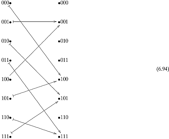
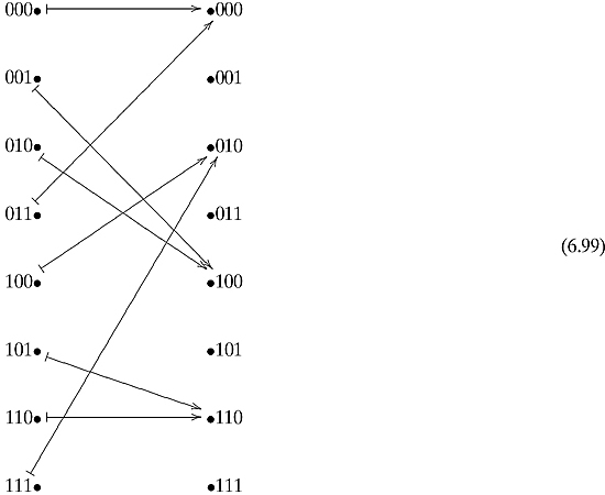
Example 6.3.1 Let us work out an example. Let n = 3. Consider c = 101. Then we are going to have the following requirements on f :

 ; hence, f (000) = f (101).

 ; hence, f (001) = f (100).

 ; hence, f (010) = f (111).

 ; hence, f (011) = f (110).

 ; hence, f (100) = f (001).

 ; hence, f (101) = f (000).

 ; hence, f (110) = f (011).

  hence, f (111) = f (010).

Exercise 6.3.1 Work out the requirements on f if c = 011.

Notice that if c = 0ⁿ, then the function is one to one. Otherwise the function is two to one.

The function f will be given as a unitary operation that can be visualized as

where goes to . U_f is again its own inverse. Setting y = 0ⁿ would give us an easy way to evaluate f (x).

How would one solve this problem classically? We would have to evaluate f on different binary strings. After each evaluation, check to see if that output has already been found. If one finds two inputs x₁ and x₂ such that f (x₁) = f (x₂), then we are assured that

and can obtain c by both sides with x₂:

If the function is a two-to-one function, then we will not have to evaluate more than half the inputs before we get a repeat. If we evaluate more than half the strings and still cannot find a match, then we know that f is one to one and that c = 0ⁿ. So, in the worst case, function evaluations will be needed. Can we do better?

The quantum part of Simon’s algorithm basically consists of performing the following operations several times:

In terms of matrices this is

Let us look at the states of the system. We start at

We then place the input in a superposition of all possible inputs. From Equation (6.63) we know that it looks like

Evaluation of f on all these possibilities gives us

And finally, let us apply to the top output, as in Equation (6.64):

Notice that for each input x and for each z, we are assured by the one who gave us the function that the ket is the same ket as . The coefficient for this ket is then

Let us examine this coefficient in depth. We saw that is an inner product and from Equation (6.57)

So, if , the terms of the numerator of this coefficient will cancel each other out and we would get . In contrast, if , the sum will be . Hence, upon measuring the top qubits, we will only find those binary strings such that .

This algorithm becomes completely clear only after we look at a concrete example.

 

---

Reader Tip. Warning: admittedly, working out all the gory details of an example can be a bit scary. We recommend that the less meticulous reader move on to the next section for now. Return to this example on a calm sunny day, prepare a good cup of your favorite tea or coffee, and go through the details: the effort will pay off.

---

 

Consider the function f :{0, 1}³ → {0, 1}³ defined as

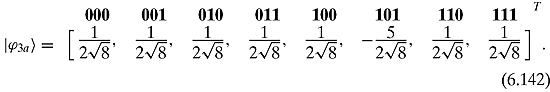
Let us go through the states of the algorithm with this function:

We might also write this as

After applying U_f , we have

or

Then applying we get

This amounts to

Notice that the coefficients follow the exact pattern as on page 184.

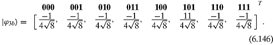
Evaluating the function f gives us

Combining like terms and canceling out gives us

or

When we measure the top output, we will get, with equal probability, 000, 010, 101, or 111. We know that for all these, the inner product with the missing c is 0. This gives us the set of equations:

 

(i)

(ii)

(iii)

(iv) .

If we write c as c = c₁c₂c₃, then Equation (ii) tells us that c₂ =0. Equation (iii) tells us that or that either c₁ = c₃ = 0 or c₁ = c₃ =1. Because we know that c≠ 000, we come to the conclusion that c = 101.

Exercise 6.3.2 Do a similar analysis for the function f defined as

After running Simon’s algorithm several times, we will get n different z_i such that . We then put these results into a classical algorithm that solves “linear equations.” They are linear equations; rather than using the usual + operation, we use on binary strings. Here is a nice worked-out example.

Example 6.3.2 Imagine that we are dealing with a case where n = 7. That means we are given a function f : {0, 1}⁷ → {0, 1}⁷. Let us assume that we ran the algorithm 7 times and we get the following results:

 

(i)

(ii)

(iii)

(iv)

(v)

(vi)

(vii) .

To clear the first column of 1’s, we are going to “add” (really pointwise exclusive or) the first equation to the third equation. This gives us

 

(i)

(ii)

(iii)

(iv)

(v)

(vi)

(vii) .

To clear the second column of 1’s, we are going to “add” the third equation to the fifth and seventh equations. This gives us

 

(i)

(ii)

(iii)

(iv)

(v)

(vi)

(vii) .

To clear the third column of 1’s, we are going to “add” the second equation to Equations (i), (iii), (iv), (v), and (vi). This gives us

 

(i)

(ii)

(iii)

(iv)

(v)

(vi)

(vii) .

To clear the fourth column of 1’s, we are going to “add” Equation (iv) to Equations (v) and (vi). We are going to clear the fifth column by adding Equation (vii) to Equation (i). This gives us

 

(i)

(ii)

(iii)

(iv)

(v)

(vi)

(vii) .

And finally, to clear the sixth column of 1’s, we are going to “add” Equation (v) to Equations (i), (ii), and (vi). We get

 

(i)

(ii)

(iii)

(iv)

(v)

(vi)

(vii) .

We can interpret these equations as

 

(i)

(ii) c₃ = 0

(iii)

(iv)

(v) c₇ = 0

(vi)

(vii) c₅ = 0.

Notice that if c₆ =0, then c₁ = c₂ = c₄ =0 and that if c₆ =1, then c₁ = c₂ = c₄ =1. Because we are certain that f is not one to one and c≠ 0000000, we can conclude that c = 1101010.

Exercise 6.3.3 Solve the following linear equations in a similar manner:

 

(i)

(ii)

(iii)

(iv)

(v)

(vi)

(vii)

(viii) .

(Hint: The answer is c = 10011001.)

In conclusion, for a given periodic f, we can find the period c in n function evaluations. This is in contrast to the 2ⁿ−¹ + 1 needed with the classical algorithm.

 

---

Reader Tip. We shall see this concept of finding the period of a function in Section 6.5 when we present Shor’s algorithm.

---

 

6.4 GROVER’S SEARCH ALGORITHM

How do you find a needle in a haystack? You look at each piece of hay separately and check each one to see if it is the desired needle. That is not very efficient. The computer science version of this problem is about unordered arrays instead of haystacks. Given an unordered array of melements, find a particular element. Classically, in the worst case, this takes mqueries. On average, we will find the desired element in m/2 queries. Can we do better?

Lov Grover’s search algorithm does the job in queries. Although this is not the exponential speedup of the Deutsch–Jozsa algorithm and Simon’s algorithm, it is still very good. Grover’s algorithm has many applications to database theory and other areas.

Because, over the past few sections, we have become quite adept at functions, let us look at the search problem from the point of view of functions. Imagine that you are given a function f: (0, 1}ⁿ → {0, 1} and you are assured that there exists exactly one binary string x₀ such that

We are asked to find x₀. Classically, in the worst case, we would have to evaluate all 2ⁿ binary strings to find the desired x₀. Grover’s algorithm will demand only evaluations.

f will be given to us as the unitary matrix U_f that takes to . For example, for n = 2, if f is the unique function that “picks out” the binary string 10, then U_f looks like

Exercise 6.4.1 Find the matrices that correspond to the other three functions from (0, 1}² to (0, 1} that have exactly one element x with f(x) =1.

As a first try at solving this problem, we might try placing into a superposition of all possible strings and then evaluating U_f.

In terms of matrices this becomes

The states are

and

Measuring the top qubits will, with equal probability, give one of the 2ⁿ binary strings. Measuring the bottom qubit will give with probability , and with probability . If you are lucky enough to measure on the bottom qubit, then, because the top and the bottom are entangled, the top qubit will have the correct answer. However, it is improbable that you will be so lucky. We need something new.

Grover’s search algorithm uses two tricks. The first, called phase inversion, changes the phase of the desired state. It works as follows. Take U_f and place the bottom qubit in the superposition

state. This is similar to quantum circuit (6.21). For an arbitrary x, this looks like

In terms of matrices this becomes

Because both U_f and H are unitary operations, it is obvious that phase inversion is a unitary operation.

The states are

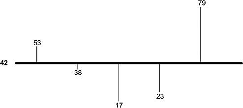
Figure 6.1. Five numbers and their average

and

Remembering that a − b = (−1)(b − a), we may write

How does this unitary operation act on states? If starts off in a equal superposition of four different states, i.e., , and f chooses the string “10,” then after performing a phase inversion, the state looks like . Measuring does not give any information: both and are equal to Changing the phase from positive to negative separates the phases, but does not separate them enough. We need something else.

What is needed is a way of boosting the phase separation of the desired binary string from the other binary strings. The second trick is called inversion about the mean or inversion about the average. This is a way of boosting the separation of the phases. A small example will be helpful. Consider a sequence of integers: 53, 38, 17, 23, and 79. The average of these numbers is a = 42. We might picture these numbers as in Figure 6.1.

The average is the number such that the sum of the lengths of the lines above the average is the same as the sum of the lengths of the lines below. Suppose we wanted to change the sequence so that each element of the original sequence above the average would be the same distance from the average but below. Furthermore, each element of the original sequence below the average would be the same distance from the average but above. In other words, we are inverting each element around the average. For example, the first number, 53 is a− 53 = −11 units away from the average. We must add a = 42 to −11 and get a + (a− 53) = 31. The second element of the original sequence, 38, is a− 38 = 4 units below the average and will go to

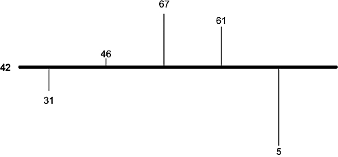
Figure 6.2. After an inversion about the mean.

a + (a− 38) = 46. In general, we shall change each element vto

or

The above sequence becomes 31, 46, 67, 61, and 5. Notice that the average of this sequence remains 42 as in Figure 6.2.

Exercise 6.4.2 Consider the following number: 5, 38, 62, 58, 21, and 35. Invert these numbers around their mean.

Let us write this in terms of matrices. Rather than writing the numbers as a sequence, consider a vector V = [53, 38, 17, 23, 79]^T. Now consider the matrix

It is easy to see that A is a matrix that finds the average of a sequence:

In terms of matrices, the formula υ′ = −υ + 2a becomes

Let us calculate

And, as expected,

or in our case,

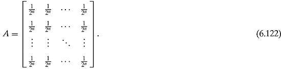
Let us generalize: rather than dealing with five numbers, let us deal with 2ⁿ numbers. Given nqubits, there are 2ⁿ possible states. A state is a 2ⁿ vector. Consider the following 2ⁿ-by-2ⁿ matrix:

Exercise 6.4.3 Prove that A² = A.

Multiplying any state by A will give a state where each amplitude will be the average of all the amplitudes. Building on this, we form the following 2ⁿ-by-2ⁿ matrix

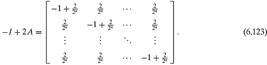
Multiplying a state by −I +2A will invert amplitudes about the mean.

We must show that −I +2A is a unitary matrix. First, observe that the adjoint of −I +2A is itself. Then, using the properties of matrix multiplication and realizing that matrices act very much like polynomials, we have

where the first equality is from distributivity of matrix multiplication, the second equality comes from combining like terms, and the third equality is from the fact that A² = A. We conclude that (−I + 2A) is a unitary operation and acts on states by inverting the numbers about the mean.

When considered separately, phase inversion and inversion about the mean are each innocuous operations. However, when combined, they are a very powerful operation that separates the amplitude of the desired state from those of all the other states.

Example 6.4.1 Let us do an example that shows how both these techniques work together. Consider the vector

We are always going to perform a phase inversion to the fourth of the five numbers. There is no difference between the fourth number and all the other numbers. We start by doing a phase inversion to the fourth number and get

The average of these five numbers is a = 6. Calculating the inversion about the mean we get

and

Thus, our five numbers become

The difference between the fourth element and all the others is 22 − 2 = 20.

Let us do these two operations again to our five numbers. Another phase inversion on the fourth element gives us

The average of these numbers is a = −2.8. Calculating the inversion about the mean we get

and

Hence, our five numbers become

The difference between the fourth element and all the others is 16.4 + 7.6=24. We have further separated the numbers. This was all done with unitary operations.

Exercise 6.4.4 Do the two operations again on this sequence of five numbers. Did our results improve?

How many times should these operations be done? times. If you do it more than that, the process will “overcook” the numbers. The proof that times is needed is beyond this text. Suffice it to say that the proof actually uses some very pretty geometry (well worth looking into!).

 

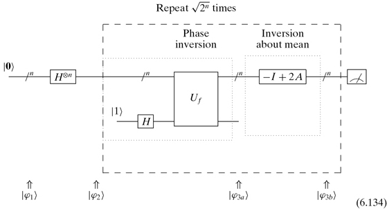
We are ready to state Grover’s algorithm:

Step 1. Start with a state

Step 2. Apply

Step 3. Repeat times:

Step 3a. Apply the phase inversion operation:

Step 3b. Apply the inversion about the mean operation:−I + 2A

Step 4. Measure the qubits.

 

We might view this algorithm as

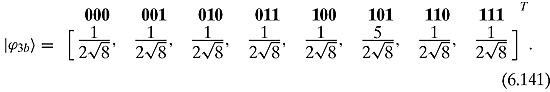
Example 6.4.2 Let us look at an example of an execution of this algorithm. Let f be a function that picks out the string “101.” The states after each step will be

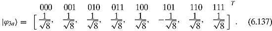
The average of these numbers is

Calculating the inversion about the mean we have

and

Thus, we have

A phase inversion will give us

The average of these numbers is

Calculating for the inversion about the mean we have

and

Hence, we have

For the record, and . Squaring the numbers gives us the probability of measuring those numbers. When we measure the state in Step 4, we will most likely get the state

which is exactly what we wanted.

Exercise 6.4.5 Do a similar analysis for the case where n = 4 and f chooses the “1101” string.

A classical algorithm will search an unordered array of size n in n steps. Grover’s algorithm will take time . This is what is referred to as a quadratic speedup. Although this is very good, it is not the holy grail of computer science: an exponential speedup. In the next section we shall meet an algorithm that does have such a speedup.

What if we relax the requirements that there be only one needle in the haystack? Let us assume that there are t objects that we are looking for (with ). Grover’s algorithm still works, but now one must go through the loop times. There are many other types of generalizations and assorted changes that one can do with Grover’s algorithm. Several references are given at the end of the chapter. We discuss some complexity issues with Grover’s algorithm at the end of Section 8.3.

6.5 SHOR’S FACTORING ALGORITHM

The problem of factoring integers is very important. Much of the World Wide Web’s security is based on the fact that it is “hard” to factor integers on classical computers. Peter Shor’s amazing algorithm factors integers in polynomial time and really brought quantum computing into the limelight.

Shor’s algorithm is based on the following fact: the factoring problem can be reduced to finding the period of a certain function. In Section 6.3 we learned how to find the period of a function. In this section, we employ some of those periodicity techniques to factor integers.

We shall call the number we wish to factor N. In practice, N will be a large number, perhaps hundreds of digits long. We shall work out all the calculations for the numbers 15 and 371. For exercises, we ask the reader to work with the number 247. We might as well give away the answer and tell you that the only nontrivial factors of 247 are 19 and 13.

We assume that the given N is not a prime number but is a composite number. There now exists a deterministic, polynomial algorithm that determines if N is prime (Agrawal, Kayal, and Saxena, 2004). So we can easily check to see if N is prime before we try to factor it.

 

---

Reader Tip. There are several different parts of this algorithm and it might be too much to swallow in one bite. If you are stuck at a particular point, may we suggest skipping to the next part of the algorithm. At the end of this section, we summarize the algorithm.

---

 

Modular Exponentiation. Before we go on to Shor’s algorithm, we have to remind ourselves of some basic number theory. We begin by looking at some modular arithmetic. For a positive integer N and any integer a, we write a Mod N for the remainder (or residue) of the quotient a/N. (For C/C++ and Java programmers, Mod is recognizable as the % operation.)

Example 6.5.1 Some examples:

7 Mod 15 = 7 because 7/15 = 0 remainder 7.

99 Mod 15 = 9 because 99/15 = 6 remainder 9.

199 Mod 15 = 4 because 199/15 = 13 remainder 4.

5,317 Mod 371 = 123 because 5,317/371 = 14 remainder 123.

2,3374 Mod 371 = 1 because 2,3374/371 = 63 remainder 1.

1,446 Mod 371 = 333 because 1,446/371 = 3 remainder 333.

Exercise 6.5.1 Calculate

 

(i) 244,443 Mod 247

(ii) 18,154 Mod 247

(iii) 226,006 Mod 247.

We write

or equivalently, if N is a divisor of a− a′, i.e., N|(a− a′).

Example 6.5.2 Some examples:

17 ≡ 2 Mod 15

126 ≡ 1,479,816 Mod 15

534 ≡ 1,479 Mod 15

2,091 ≡ 236 Mod 371

3,350 ≡ 2237 Mod 371

3,325,575 ≡ 2,765,365 Mod 371.

Exercise 6.5.2 Show that

(i) 1,977 ≡ 1 Mod 247

(ii) 16,183 ≡ 15,442 Mod 247

(iii) 2,439,593 ≡ 238,082 Mod 247.

With Mod understood we can start discussing the algorithm. Let us randomly choose an integer a that is less than N but does not have a nontrivial factor in common with N. One can test for such a factor by performing Euclid’s algorithm to calculate GCD(a, N). If the GCD is not 1, then we have found a factor of N and we are done. If the GCD is 1, then a is called co-prime to N and we can use it. We shall need to find the powers of a modulo N, that is,

In other words, we shall need to find the values of the function

Some examples are in order.

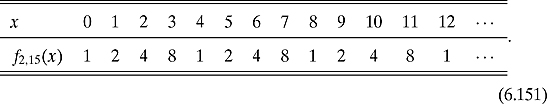
Example 6.5.3 Let N = 15 and a = 2. A few simple calculations show that we get the following:

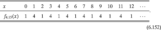
For a = 4, we have

For a = 13, we have

The first few outputs of f_{13, 15} function can be viewed as the bar graph in Figure 6.3.

Example 6.5.4 Let us work out some examples with N = 371. This is a little harder and probably cannot be done with a handheld calculator. The numbers simply get too large. However, it is not difficult to write a small program, use MATLAB or Microsoft Excel. Trying to calculate a^x Mod N by first calculating a^x will not go very far, because the numbers will usually be beyond range. Rather, the trick is to calculate a^x Mod N from a^x−¹ Mod N by using the standard number theoretic fact

Figure 6.3. The first few outputs of f_{13, 15}.

that

Or, equivalently

From this fact we get the formula

Because a < N and a Mod N=a, this reduces to

Using this, it is easy to iterate to get the desired results. For N = 371 and a = 2, we have

For N = 371 and a = 6, we have

Figure 6.4. The output of f_24,371.

For N = 371 and a = 24, we have

We can see the results of f_{24, 371} as a bargraph in Figure 6.4.

Exercise 6.5.3 Calculate the first few values of f_{a, N} for N = 247 and

(i) a = 2

(ii) a = 17

(iii) a = 23.

In truth, we do not really need the values of this function, but rather we need to find the period of this function, i.e., we need to find the smallest r such that

It is a theorem of number theory that for any co-prime a≤ N, the function f_{a, N} will output a 1 for some r < N. After it hits 1, the sequence of numbers will simply repeat. If f_{a, N}(r) = 1, then

and in general

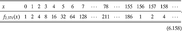
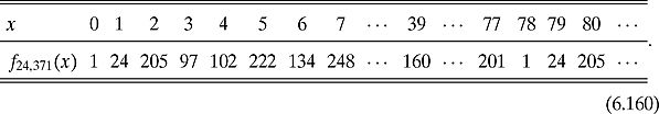
Example 6.5.5 Charts (6.151), (6.152), and (6.153) show us that the periods for f₂,₁₅, f₄,₁₅, and f₁₃,₁₅ are 4, 2, and 4, respectively. Charts (6.158), (6.159), and (6.160) show us that the periods for f₂,₃₇₁, f₆,₃₇₁, and f₂₄,₃₇₁ are 156, 26, and 78, respectively. In fact, it is easy to see the periodicity of f₂₄,₃₇₁ in Figure 6.4.

Exercise 6.5.4 Find the period of the functions f₂,₂₄₇, f₁₇,₂₄₇, and f₂₃,₂₄₇.

The Quantum Part of the Algorithm. For small numbers like 15, 371, and 247, it is fairly easy to calculate the periods of these functions. But what about a large N that is perhaps hundreds of digits long? This will be beyond the ability of any conventional computers. We will need a quantum computer with its ability to be in a superposition to calculate f_a,_N(x) for all needed x.

How do we get a quantum circuit to find the period? First we have to show that there is a quantum circuit that can implement the function f_a,_N. The output of this function will always be less than N, and so we will need n = log₂ N output bits. We will need to evaluate f_a,_N for at least the first N² values of x and so will need at least

input qubits. The quantum circuit that we would get will be the operator U_fa,_N, which we may visualize as

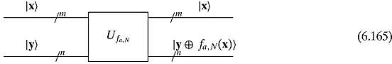
where goes to .² How is this circuit formed? Rather than destroying the flow of the discussion, we leave that technical discussion for a mini appendix at the end of this section.

With U_fa,N, we can go on to use it in the following quantum algorithm. The first thing is to evaluate all the input at one time. From earlier sections, we know how to put x into an equally weighted superposition. (In fact, the beginning of this algorithm is very similar to Simon’s algorithm.) We shall explain all the various parts of this quantum circuit:

In terms of matrices this is

where 0_m and 0_n are qubit strings of length m and n, respectively. Let us look at the states of the system. We start at

We then place the input in an equally weighted superposition of all possible inputs:

Evaluation of f on all these possibilities gives us

As the examples showed, these outputs repeat and repeat. They are periodic. We have to figure out what is the period. Let us meditate on what was just done. It is right here where the fantastic power of quantum computing is used. We have evaluated all the needed values at one time! Only quantum parallelism can perform such a task.

Let us pause and look at some examples.

Example 6.5.6 For N = 15, we will have n = 4 and m = 8. For a = 13, the state will be

Example 6.5.7 For N = 371, we will have n = 9 and m = 18. For a = 24, the state will be

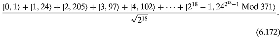
Exercise 6.5.5 Write the state for N = 247 and a = 9.

Going on with the algorithm, we measure the bottom qubits of , which is in a superposition of many states. Let us say that after measuring the bottom qubits we find

for some . However, by the periodicity of f_a,N we also have that

and

In fact, for any we have

How many of the 2^m superpositions x in have Mod N as the output? Answer: . So

We might also write this as

where t₀ is the first time that Mod N, i.e., the first time that the measured value occurs. We shall call t₀ the offset of the period for reasons that will soon become apparent.

It is important to realize that this stage employs entanglement in a serious fashion. The top qubits and the bottom qubits are entangled in a way that when the top is measured, the bottom stays the same.

Example 6.5.8 Continuing Example 6.5.6, let us say that after measurement of the bottom qubits, 7 is found. In that case would be

For example, if we looked at the f₁₃,₁₅ rather than the bargraph in Figure 6.3, we would get the bargraph shown in Figure 6.5.

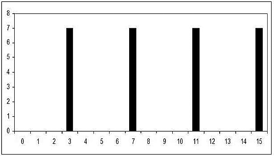
Figure 6.5. f₁₃,₁₅ after a measurement of 7.

Example 6.5.9 Continuing Example 6.5.7, let us say that after measurement of the bottom qubits we find 222 (which is 24⁵ Mod 371.) In that case would be

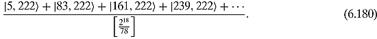
We can see the result of this measurement in Figure 6.6

Exercise 6.5.6 Continuing Exercise 6.5.5, let us say that after measuring the bottom qubits, 55 is found. What would be?

The final step of the quantum part of the algorithm is to take such a superposition and return its period. This will be done with a type of Fourier transform. We do not

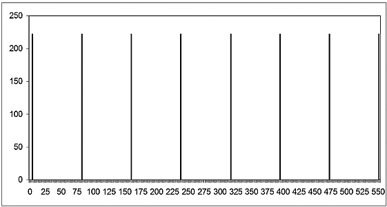
Figure 6.6. f_24,371 after a measurement of 222.

assume the reader has seen this before and some motivation is in order. Let us step away from our task at hand and talk about evaluating polynomials. Consider the polynomial

We can represent this polynomial with a column vector [a₀, a₁, a₂, … a_n−1]^T. Suppose we wanted to evaluate this polynomial at the numbers x₀, x₁, x₂, … x_n−1, i.e., we wanted to find P(x₀), P(x₁), P(x₂), … , P(x_n−1). A simple way of performing the task is with the following matrix multiplication:

The matrix on the left, where every row is a geometric series, is called the Vandermonde matrix and is denoted (x₀, x₁, x₂, x_n−1). There is no restriction on the type of numbers we are permitted to use in the Vandermonde matrix, and hence, we are permitted to use complex numbers. In fact, we shall need them to be powers of the Mth roots of unity, ω_M (see page 26 of Chapter 1 for a quick reminder). Because M is fixed throughout this discussion, we shall simply denote this as ω. There is also no restriction on the size of the Vandermonde matrix. Letting M =2^m, which is the amount of numbers that can be described with the top qubits, there is a need for the Vandermonde matrix to be an M-by-M matrix. We would like to evaluate the polynomials at ω⁰ =1, ω, ω² , … , ω^M−1. To do this, we need to look at (ω⁰, ω¹, ω², … , ω^M−1). In order to evaluate P(x) at the powers of the Mth root of unity, we must multiply

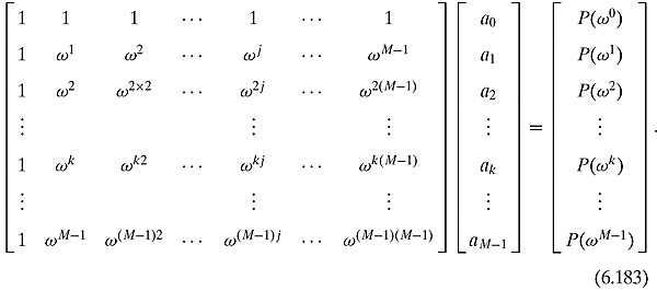
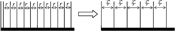
Figure 6.7. The action of DFT^†.

[P(ω⁰), P(ω¹), P(ω²),…, P(ω^k),…, P(ω^M−1)]^T is the vector of the values of the polynomial at the powers of the Mth root of unity.

Let us define the discrete Fourier transform, denoted DFT, as

Formally, DFT is defined as

It is easy to see that DFT is a unitary matrix: the adjoint of this matrix, DFT^†, is formally defined as

To show that DFT is unitary, let us multiply

If k = j, i.e., if we are along the diagonal, this becomes

If k≠ j, i.e., if we are off the diagonal, then we get a geometric progression which sums to 0. And so DFT * DFT^† = I.

What task does DFT† perform? Our text will not get into the nitty-gritty of this important operation, but we shall try to give an intuition of what is going on. Let us forget about the normalization for a moment and think about this intuitively. The matrix DFT acts on polynomials by evaluating them on different equally spaced points of the circle. The outcomes of those evaluations will necessarily have periodicity because the points go around and around the circle. So multiplying a column vector with DFT takes a sequence and outputs a periodic sequence. If we start with a periodic column vector, then the DFT will transform the periodicity. Similarly, the inverse of the Fourier transform, DFT^†, will also change the periodicity. Suffice it to say that the DFT^† does two tasks as shown in Figure 6.7:

It modifies the period from r to

It eliminates the offset.

Circuit (6.166) requires a variant of a DFT called a quantum Fourier transform and denoted as QFT. Its inverse is denoted QFT^†. The QFT^†performs the same operation but is constructed in a way that is more suitable for quantum computers. (We shall not delve into the details of its construction.) The quantum version is very fast and made of “small” unitary operators that are easy for a quantum computer to implement.³

The final step of the circuit is to measure the top qubits. For our presentation, we shall make the simplifying assumption that r evenly divides into 2^m. Shor’s actual algorithm does not make this assumption and goes into details about finding the period for any r. When we measure the top qubit we will find it to be some multiple of . That is, we will measure

for some whole number λ. We know 2^m, and after measuring we will also know x. We can divide the whole number x by 2^m and get

One can then reduce this number to an irreducible fraction and take the denominator to be the long sought-after r. If we do not make the simplifying assumption that r evenly divides into 2^m, then we might have to perform this process several times and analyze the results.

From the Period to the Factors. Let us see how knowledge of the period r will help us find a factor of N. We shall need a period that is an even number. There is a theorem of number theory that tells us that for the majority of a, the period of f_a,N will be an even number. If, however, we do choose an a such that the period is an odd number, simply throw that a away and choose another one. Once an even r is found so that

we may subtract 1 from both sides of the equivalence to get

or equivalently

Remembering that 1=1² and x² −y² =(x+y)(x−y) we get that

or

(If r was odd, we would not be able to evenly divide by 2.) This means that any factor of N is also a factor of either or both. Either way, a factor for N can be found by looking at

and

Finding the GCD can be done with the classical Euclidean algorithm. There is, however, one caveat. We must make sure that

because if Mod N, then the right side of Equation (6.197) would be 0. In that case we do not get any information about N and must throw away that particular a and start over again.

Let us work out some examples.

Example 6.5.10 In chart (6.151), we saw that the period of f₂,₁₅ is 4, i.e., 2⁴ ≡ 1 Mod 15. From Equation (6.197), we get that

And, hence, we have that GCD(5, 15) = 5 and GCD(3, 15) = 3.

Example 6.5.11 In chart (6.159), we saw that the period of f₆,₃₇₁ is 26, i.e., 6²⁶ ≡1 Mod 371. However, we can also see that . So we cannot use a = 6.

Example 6.5.12 In chart (6.160), we saw that the period of f₂₄,₃₇₁ is 78, i.e., 24⁷⁸ ≡ 1 Mod 371. We can also see that Mod 371. From Equation (6.197), we get that

And, thus, GCD(161, 371) = 7 and GCD(159, 371) = 53 and 371 = 7 _* 53.

Exercise 6.5.7 Use the fact that the period of f₇,₂₄₇ is 12 to determine the factors of 247.

Shor’s Algorithm. We are, at last, ready to put all the pieces together and formally state Shor’s algorithm:

Input: A positive integer N with n = [log₂ N].

Output: A factor p of N if it exists.

Step 1. Use a polynomial algorithm to determine if N is prime or a power of prime. If it is a prime, declare that it is and exit. If it is a power of a prime number, declare that it is and exit.

Step 2. Randomly choose an integer a such that 1 < a< N. Perform Euclid’s algorithm to determine GCD(a, N). If the GCD is not 1, then return it and exit.

Step 3. Use quantum circuit (6.166) to find a period r.

Step 4. If r is odd or if a^r ≡ −1 Mod N, then return to Step 2 and choose another a.

Step 5. Use Euclid’s algorithm to calculate and . Return at least one of the nontrivial solutions.

What is the worst case complexity of this algorithm? To determine this, one needs to have an in-depth analysis of the details of how U_a,_N and QFT^† are implemented. One would also need to know what percentage of times things can go wrong. For example, what percentage of a would f_a,N have an odd period? Rather than going into the gory details, let us just state that Shor’s algorithm works in

number of steps, where n is the number of bits needed to represent the number N. That is polynomial in terms of n. This is in contrast to the best-known classical algorithms that demand

steps, where c is some constant. This is exponential in terms of n. Shor’s quantum algorithm is indeed faster.

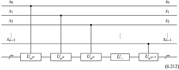
Appendix: Implementing U_fa,N with quantum gates. In order for U_fa,N to be implemented with unitary matrices, we need to “break up” the operations into small little jobs. This is done by splitting up x. Let us write x in binary. That is,

Formally, x as a number is

Using this description of x, we can rewrite our function as

or

We can convert this formula to an inductive definition⁴ of f_a,N(x). We shall define y₀, y₁, y₂,…, y_n−2, y_n−1, where y_n−1 = f_a,N(x): the base case is

If we have y_j−1, then to get y_j we use the trick from Equation (6.157):

Notice that if x_j = 0 then y_j = y_j−1. In other words, whether or not we should multiply y_j−1 by a^2j Mod N is dependent on whether or not x_j =1. It turns out that as long as a and N are co-prime, the operation of multiplying a number times a^2j Mod N is reversible and, in fact, unitary. So for each j, there is a unitary operator

that we shall write as U_a^2j . As we want to perform this operation conditionally, we will need controlled-U_a^2j , or ^CU_a^2j, gates. Putting this all together, we have the following quantum circuit that implements f_a,_N in a polynomial number of gates:

Even if a real implementation of large-scale quantum computers is years away, the design and study of quantum algorithms is something that is ongoing and is an exciting field of interest.

 

---

References:

(i) A version of Deutsch’s algorithm was first stated in Deutsch (1985).

(ii) Deutsch–Jozsa was given in Deutsch and Jozsa (1992).

(iii) Simon’s algorithm was first presented in Simon (1994).

(iv) Grover’s search algorithm was originally presented in Grover (1997). Further developments of the algorithm can be found in Chapter 6 of Nielsen and Chuang (2000). For nice applications of Grover’s algorithm to graph theory, see Cirasella (2006).

(v) Shor’s algorithm was first announced in Shor (1994). There is also a very readable presentation of it in Shor (1997). There are several slight variations to the algorithm and there are many presentations at different levels of complexity. Chapter 5 of Nielsen and Chuang (2000) goes through it thoroughly. Chapter 10 of Dasgupta, Papadimitriou, and Vazirani (2006) goes from an introduction to quantum computing through Shor’s algorithm in 20 pages.

Every quantum computer textbook works through several algorithms. See, e.g., Hirvensalo (2001) and Kitaev, Shen, and Vyalyi (2002) and, of course, Nielsen and Chuang (2000). There is also a very nice short article by Shor that discusses several algorithms (Shor, 2002). Dorit Aharonov has written a nice survey article that goes through many of the algorithms (Aharonov, 1998)

Peter Shor has written a very interesting article on the seeming paucity of quantum algorithms in Shor (2003).

¹ This is reminiscent of the definition of an inner product. In fact, it is an inner product, but on an interesting vector space. The vector space is not a complex vector space, nor a real vector space. It is a vector space over the field with exactly two elements {0, 1}. This field is denoted or . The set of elements of the vector space is {0,1}ⁿ, the set of bit strings of length n, and the addition is pointwise . The zero element is the string of nzeros. Scalar multiplication is obvious. We shall not list all the properties of this inner product space but we strongly recommend that you do so. Meditate on a basis and on the notions of orthogonality, dimension, etc.

² Until now, we have thought of x as any number and now we are dealing with x as its binary expansion x. This is because we are thinking of x as described in a (quantum) computer. We shall use both notations interchangeably

³ There are slight variations of Shor’s algorithm: For one, rather than using the to put the m qubits in a superposition in the beginning of circuit (6.166), we could have used QFT and get the same results. However, we leave it as is because at this point the reader has familiarity with the Hadamard matrix. Another variation is not measuring the bottom qubits before performing the QFT^† operation. This makes the mathematics slightly more complicated. We leave it as is for simplicity sakes. However, if we take both of these variants, our quantum circuit would look like

This would have been more in line with our discussion at the end of Section 2.3, where we wrote about solving problems using

where QFT and QFT^† would be our two translations.

⁴ This inductive definition is nothing more than the modular-exponentiation algorithm given in, say, Section 31.6 of Corman et al. (2001) or Section 1.2 of Dasgupta, Papadimitriou, and Vazirani (2006).