10

Information Theory

---

 

 

 

 

I find that a great part of the information I have was acquired by looking up something and finding something else on the way.

Franklin P. Adams

The topic of this chapter is quantum information, i.e., information in the quantum world. The material that is presented here lies at the core of a variety of areas within the compass of quantum computation, such as quantum cryptography, described in Chapter 9, and quantum data compression. As quantum information extends and modifies concepts developed in classical information theory, a brief review of the mathematical notion of information is in order.

In Section 10.1, we recall the basics of classical information theory. Section 10.2 generalizes this work to get quantum information theory. Section 10.3 discusses classical and quantum data compression. We conclude with a small section on error-correcting codes.

10.1 CLASSICAL INFORMATION AND SHANNON ENTROPY

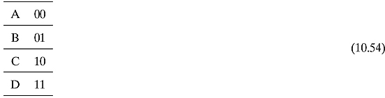
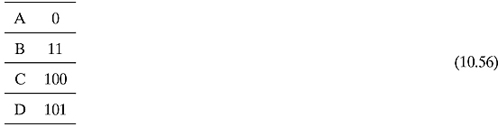
What is information really? In the mid-forties, an American mathematician named Claude Shannon set out to establish a mathematical theory of information on a firm basis. To see this, we use Alice and Bob. Alice and Bob are exchanging messages. Let us say that Alice can only send one of four different messages coded by the letters A, B, C, and D.

In our story, the meaning of the four letters is as following:

Figure 10.1. Three possible probability distributions.

Bob is a careful listener, so he keeps track of the frequency of each letter. By observing N consecutive messages from Alice, he reports the following:

 

A appeared N_A times

B appeared N_B times

C appeared N_C times

D appeared N_D times

where N_A + N_B + N_C + N_D = N. Bob concludes that the probability of each letter showing up is given by

The table that associates with each basic symbol its probability is known as the probability distribution Function (pdf for short) of the source. Of course, the probability distribution may have different shapes (Figure 10.1). For instance, Alice may be always happy (or at least say so to Bob), so that the pdf looks like

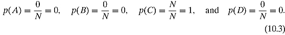
Such a pdf is called the constant distribution. In this case, Bob knows with certainty that the next symbol he will receive from Alice is C. It stands to reason that in this scenario C does not bring any new information: its information content is zero.

On the opposite side of the spectrum, let us assume that Alice is very moody, in fact totally unpredictable, as far as her emotional state goes. The pdf will then look like

Such a pdf is called the uniform distribution. In this case, when Bob will observe the new symbol from Alice, he will gain information, indeed the maximum amount of information this limited alphabet could convey.

These two scenarios are just two extremes among infinitely many others. For instance, the pdf might look like

It is quite obvious that this general scenario stands in between the other two, in the sense that its outcome is less certain than the one afforded by the constant pdf, but more so than the uniform pdf.

We have just found a deep connection between uncertainty and information. The more uncertain the outcome, the more Bob will gain information by knowing the outcome. What Bob can predict beforehand does not count: only novelty brings forth information!¹ The uniform probability distribution represents the greatest uncertainty about the outcome: everything can happen with equal likelihood; likewise, its information content is the greatest.

It now becomes clear what we need: a way to quantify the amount of uncertainty in a given probability distribution. Shannon, building on classical statistical thermodynamics, introduced precisely such a measure.

Definition 10.1.1 The Shannon entropy of a source with probability distribution{p_i} is the quantity

where the following convention has been adopted: 0 × log₂(0) = 0.²

Note: The minus sign is there to make sure that entropy is always positive or zero, as shown by the following exercise.

Exercise 10.1.1 Prove that Shannon entropy is always positive or zero.

Why should we believe that the formula presented in Equation (10.6) does indeed capture the uncertainty of the source? The better course is to calculate H for each of the aforementioned scenarios above.

Let us compute the entropy for the constant pdf:

As we see, the entropy is as low as it can be, just as we would expect. When the entropy equals zero, that means there is absolutely no uncertainty in the source.

Let us move to the uniform pdf:

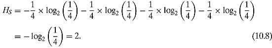
This makes sense. After all, because Bob has no real previous information, he needs no less than two bits of information to describe which letter is being sent to him.

And now the general scenario:

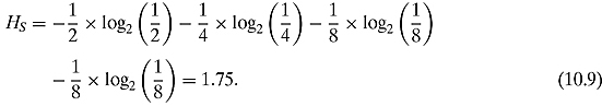
We have thus verified, at least for the preceding examples, that the entropy formula does indeed classify the amount of uncertainty of the system.

Exercise 10.1.2 Create a fourth scenario that is strictly in between the general pdf in Equation (10.9) and the uniform distribution. In other words, determine a pdf for the four-symbol source whose entropy verifies 1.75 < H< 2.

Exercise 10.1.3 Find a pdf for the four-symbol source so that the entropy will be less than 1 but strictly positive.

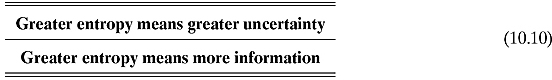
Summing up, we can recapitulate the above into two complementary slogans:

Programming Drill 10.1.1 Write a simple program that lets the user choose how many letters the source alphabet has, and then enter the probability distribution. The program should visualize it, and compute its Shannon entropy.

10.2 QUANTUM INFORMATION AND VON NEUMANN ENTROPY

The previous section dealt with the transmission of classical information, i.e., information that can be encoded as a stream of bits. We are now going to investigate to what extent things change when we are concerned with sources emitting streams of qubits.

As it turns out, there is a quantum analog of entropy, known as von Neumann entropy. Just as Shannon entropy measures the amount of order in a classical system, von Neumann entropy will gauge order in a given quantum system. Let us set the quantum scenario first. Alice has chosen as her quantum alphabet a set of normalized states in :

If she wishes to notify Bob of her moods, as in the previous section, she can choose four normalized states in some state space. Even the single qubit space is quite roomy (there are infinitely many distinct qubits), so she could select the following set:

Notice that Alice does not have to choose an orthogonal set of states, they simply need to be distinct.

Now, let us assume that she sends to Bob her states with probabilities:

We can associate with the table above a linear operator, known as the density operator,³ defined by the following expression:

D does not look like anything we have met so far. It is the weighted sum of a basic expression of the form , i.e., products of a bra with their associated ket. To get some sense for what D actually does, let us study first how its building blocks operate. acts on a ket vector in the following way:

In plain words, the result of applying to a generic ket is simply the projection of onto , as shown in Figure 10.2. The length of the projection is the scalar product (we are here using the fact that all w_i’s are normalized).

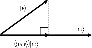
Figure 10.2. The projection of onto .

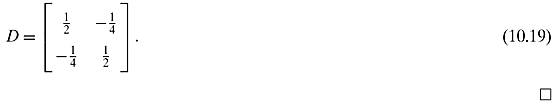
Exercise 10.2.1 Assume Alice always sends only one vector, say, w₁. Show that D in this case just looks like .

Now that we know how each component acts on a ket, it is not difficult to understand the entire action of D. It acts on ket vectors on the left:

In words, D is the sum of projections onto all the ’s, weighted by their respective probabilities.

Exercise 10.2.2 Show that the action we have just described makes D a linear operator on kets (check that it preserves sums and scalar multiplication).

As D is now a legitimate linear operator on the ket space, it can be represented by a matrix, once a basis is specified. Here is an example:

Example 10.2.1 Let and . Assume that is sent with probability and is sent with probability . Let us now describe the corresponding density matrix in the standard basis. In order to do so, we just compute the effect of D on the two basis vectors:

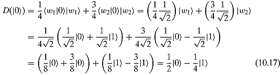
The density matrix is thus

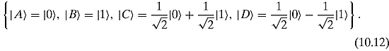
Exercise 10.2.3 Write the density matrix of the alphabet in Equation (10.12), where

D also acts on bra vectors on the right, using a mirror recipe:

What we have just found, namely, that D can operate on both bras and kets at the same time, suggests that we combine the action on the left and the right in one shot. Given any state , we can form

The meaning of the number will become apparent in a moment. Suppose Alice sends a state and Bob performs a measurement whose possible outcomes is the set of orthonormal states

Let us compute the probability that Bob observes the state .

Alice sends with probability p₁. Each time Bob receives , the probability that the outcome is is precisely . Thus is the probability that Alice has sent and Bob has observed . Similarly for . Conclusion: is the probability that Bob will see regardless of which state Alice has sent him.

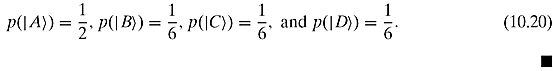
Example 10.2.2 Assume Alice has a quantum alphabet consisting of only two symbols, the vectors

and

Notice that, unlike Example 10.2.1, here the two states are not orthogonal. Alice sends with frequency and with frequency . Bob uses the standard basis for his measurements.

The density operator is

Let us write down the density matrix in the standard basis:

The density matrix is thus

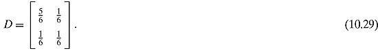
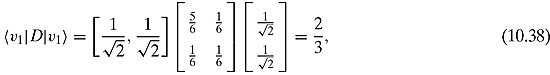
Now we can calculate and

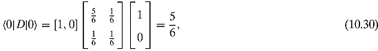
If we calculate Shannon entropy with respect to this basis, we get

Even though Alice is sending ’s, from Bob’s standpoint, the source behaves as an emitter of states

with probability distribution given by

It would be tempting to conclude that the source has entropy given by the same recipe as in the classical case:

However, things are a bit more complicated and more interesting also. Bob can choose different measurements, each associated with its own orthonormal basis. The probability distribution will change as he changes basis, as shown by the following example.

Example 10.2.3 Suppose Bob settles for the basis

Let us calculate and (the density matrix is the same as in Example 10.2.1):

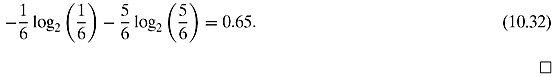
Let us calculate the Shannon entropy for this pdf:

Compared to Equation (10.32), the Shannon entropy, as perceived by Bob, has increased, because the pdf is less sharp than before. The source, however, hasn’t changed at all: quite simply, Bob has replaced his “pair of glasses” (i.e., his measurement basis) with a new one!

Exercise 10.2.4 Write the matrix of the general density operator D described by Equation 10.14 in the standard basis of , and verify that it is always hermitian. Verify that the trace of this matrix, i.e., the sum of its diagonal entries, is 1.

We can ask ourselves if there is a privileged basis, among the ones Bob can choose. Put differently, is there a basis that minimizes the calculation of Shannon entropy in Equation (10.35)? It turns out that such a basis does exist. Because the density operator is hermitian, we saw using the spectral theorem for self-adjoint operators on page 64, that it can be put in diagonal form. Assuming that its eigenvalues are

we can then define the von Neumann entropy as follows:

Definition 10.2.1 The von Neumann entropy⁴ for a quantum source represented by a density operator D is given by

where λ₁, λ₂,…, λ_n are the eigenvalues of D.

If Bob selects the basis

of orthonormal eigenvectors of D corresponding to the eigenvalues listed in Equation (10.47), the von Neumann entropy is precisely identical to the calculation of Shannon entropy in Equation (10.40) with respect to the basis of eigenvectors. Why? If you compute

you get

(we have used the orthonormality of ).

The same holds true for all eigenvectors: the eigenvalue λ_i is the probability that Bob will observe when he measures incoming states in the eigenvector basis!

Example 10.2.4 Let us continue the investigation we began in Example 10.2.2. The density matrix D has eigenvalues

corresponding to the normalized eigenvectors

The von Neumann entropy of D is given by

Let us verify that von Neumann’s entropy is identical to Shannon’s entropy when calculated with respect to the orthonormal basis of eigenvectors of D:

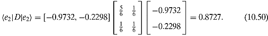
Observe that the sum of eigenvalues 0.8727 + 0.1273 is 1, and both eigenvalues are positive, as befits true probabilities. Also notice that the entropy is lower than the one calculated using the other two bases; it can indeed be proven that it is as low as it can possibly be.

Exercise 10.2.5 Go through all the steps of Examples 10.2.1, 10.2.2, and 10.2.3, assuming that Alice sends the same states, but with equal probability.

Note that for this exercise, you will need to calculate eigenvectors and eigenvalues. In Chapter 2 we stated what eigenvalues and eigenvectors are, but not how to compute them for a given symmetric or hermitian matrix. To complete this exercise, you have two equally acceptable options:

1. Look up any standard reference on linear algebra for the eigenvalues formula (search for “characteristic polynomial”).

2. Use a math library to do the work for you. In MATLAB, for instance, the function eig is the appropriate one (Mathematica and Maple come equipped with similar functions).

As we have said, Alice is at liberty in choosing her alphabet. What would happen if she selected a set of orthogonal vectors? The answer is in the following pair of exercises.

Exercise 10.2.6 Go back to Example 10.2.1. The two states and are a pair of orthonormal vectors, and thus an orthonormal basis for the one qubit space. Show that they are eigenvectors for the density matrix given in Equation (10.19), and thus Bob’s best choice for measuring incoming messages.

Exercise 10.2.7 This exercise is just the generalization of the previous one, in a more formal setting. Suppose Alice chooses from a set of orthonormal state vectors

with frequencies

to code her messages. Prove that in this scenario each of the ’s is a normalized eigenvector of the density matrix with eigenvalue p_i. Conclude that in this case the source behaves like a classical source (provided of course that Bob knows the orthonormal set and uses it to measure incoming states).

In the wake of the two foregoing exercises, we now know that orthogonal quantum alphabets are the less surprising ones. Let us go back briefly to Example 10.2.2: there Alice’s choice is a nonorthogonal set. If you calculate explicitly its von Neumann entropy, you will find that it is equal to 0.55005, whereas the classical entropy for a source of bits such that and is 0.91830.

We have just unraveled yet another distinct feature of the quantum world: if we stick to the core idea that entropy measures order, then we come to the inescapable conclusion that the quantum source above exhibits more order than its classical counterpart. Where does this order come from? If the alphabet is orthogonal, the two numbers are the same. Therefore, this apparent magic is due to the fact that there is additional room in the quantum via superposition of alternatives.⁵ Our discovery is a valuable one, also in light of the important connection between entropy and data compression, the topic of the next section.

Programming Drill 10.2.1 Write a program that lets the user choose how many qubits the alphabet of the quantum source consists of, enter the probability associated with each qubit, and compute von Neumann entropy as well as the orthonormal basis for the associated density matrix.

10.3 CLASSICAL AND QUANTUM DATA COMPRESSION

In this section, we introduce the basic ideas of data compression for bit and qubit streams. Let us begin with bits first.

What is data compression? Alice has a message represented by a stream of bits. She wants to encode it either for storage or for transmission in such a way that the encoded stream is shorter than the original message. She has two main options:

Lossless data compression, meaning that her compression algorithm must have an inverse that perfectly reconstruct her message.

Lossy data compression, if she allows a loss of information while compressing her data.

In data compression, a notion of similarity between strings is always assumed, i.e., a function that enables us to compare different strings (in our scenario, the message before compression and the one after it has been decompressed):

such that

μ(s, s) = 0 (a string is identical to itself), and

μ(s₁, s₂) = μ(s₂, s₁) (symmetry of similarity).⁶

Armed with such a notion of similarity, we can now define compression.

Definition 10.3.1 Let μ be a measure of similarity for binary strings, a fixed threshold, and len( ) the length of a binary string. A compression scheme for a given source S is a pair of functions(ENC, DEC) from the set of finite binary strings to itself, such that

len(ENC(s)) < len(s) on average, and

for all sequences.

If μ(s, DEC(ENC(s))) = 0 for all strings, then the compression scheme is lossless.

In the first item, we said “on average,” in other words, for most messages sent by the source. It is important to realize that compression schemes are always coupled with a source: if the source’s pdf changes, a scheme may become useless.

Which of the two options listed in Definition 10.3.1 is actually chosen depends on the problem at hand. For instance, if the sender wants to transmit an image, she may decide to go for lossy compression, as small detail losses hardly affect the reconstructed image.⁷ On the other hand, if she is transmitting or storing, say, the source code of a program, every single bit may count. Alice here does not have the luxury to waste bits; she must resort to lossless compression.⁸ As a rule of thumb, lossy compression allows you to achieve much greater compression (its requirements are less stringent!), so if you are not concerned with exact reconstruction, that is the obvious way to go.

There is a fundamental connection between Shannon entropy and data compression. Once again, let us build our intuition by working with the general pdf given in Section 10.1.

Note: We make an assumption throughout this section: the source is independently distributed. This simply means that each time Alice sends a fresh new symbol, the probability stays the same and there is no correlation with previous sent symbols.

Alice must transmit one of four symbols. Using the binary alphabet 0, 1, she can encode her A, B, C, D using log₂(4)=2 bits. Suppose she follows this coding

How many bits will she send on average per symbol?

Doesn’t sound too good, does it? Alice can definitely do better than that. How? The core idea is quite simple: she will use an encoding that uses fewer bits for symbols that have a higher probability. After a little thinking, Alice comes up with this encoding:

Let us now compute the average number of bits per symbol Alice is going to transmit using this encoding:

As you have already noticed, this is precisely the value we have found for the entropy of the source.

Exercise 10.3.1 Try to determine the most efficient coding for a four-symbol source whose pdf looks like

What we have just seen is far from accidental: indeed, it represents a concrete example of a general fact discovered by Shannon, namely, an entropy-related bound on how good compression can be for a given source.

Theorem 10.3.1 (Shannon’s Noiseless Channel Coding Theorem). Let a source S emit symbols from an alphabet with a given probability distribution. A message of length n, with n sufficiently large, sent over a noiseless channel can be compressed on average without loss of information to a minimum of H(S) × n bits.

We shall not provide a formal proof of Shannon’s theorem, only the underlying heuristics behind it. Imagine for simplicity’s sake that the source transmits only binary sequences. If the length n of the message is large enough, most sequences will have a distribution of 0’s and 1’s, which will approximately correspond to their respective probability. These well-behaved sequences are called typical, and all together they form a subset of all messages, known as the typical set. For instance, suppose that 1 appears with probability and 0 with probability . A typical sequence of length, say, 90, would have exactly 30 bits set to 1.

How many typical sequences are there? It turns out that their number is roughly given by 2^H(S)n. As you can see from Figure 10.3, this is a proper subset of the set of all sequences of length n (the entire set has 2ⁿ elements), as long as H< 1.

An ideal compression strategy is then the following:

Create a lookup table for all the typical sequences of length n. The key for the table needs exactly H(S)n bits. This lookup table is shared by Alice and Bob.

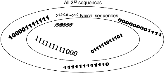
Figure 10.3. , , n = 12, H(S) = 0.81128.

When a message of length n is sent, Alice sends one bit to inform Bob that the sequence is typical, and the bits to look up the result. If the sequence is not typical, Alice sends the bit that says “not typical,” and the original sequence.

For n large enough, almost all sequences will be typical or near typical, so the average number of bits transmitted will get very close to Shannon’s bound.

Exercise 10.3.2 Assume that the source emits 0 with probability and 1 with probability . Count how many typical sequences of length n are there. (Hint: Start with some concrete example, setting n = 2, 3,…. Then generalize.)

Programming Drill 10.3.1 Write a program that accepts a pdf for 0 and 1, a given length n, and produces as output the list of all typical sequences of length n.

Note: Shannon’s theorem does not say that all sequences will be compressed, only that what the average compression rate for an optimal compression scheme will be. Indeed, a universal recipe for lossless compression of all binary sequences does not exist, as you can easily show doing the following exercise.

Exercise 10.3.3 Prove that there is no bijective map f from the set of finite binary strings to itself such that for each sequence s, length( f (s)) < length(s). (Hint: Start from a generic sequence s₀. Apply f to it. Now iterate. What happens to the series of sequences {s₀, f (s₀), f ( f (s₀)), …}?)

Shannon’s theorem establishes a bound for lossless compression algorithms, but it does not provide us with one. In some cases, as we have seen in the previous examples, we can easily find the optimal protocol by hand. In most situations though, we must resort to suboptimal protocols. The most famous and basic one is known as Huffman’s algorithm.⁹ You may have met it already in an Algorithms and Data Structures class.

Figure 10.4. Alice sending messages to Bob in a four-qubit alphabet.

Programming Drill 10.3.2 Implement Huffman’s algorithm, and then experiment with it by changing the pdf of the source. For which source types does it perform poorly?

It is now time to discuss qubit compression. As we already mentioned in the beginning of Section 10.3, Alice is now emitting sequences of qubits with certain frequencies to send her messages. More specifically, assume that Alice draws from a qubit alphabet of k distinct but not necessarily orthogonal qubits, with frequency p₁,…,p_k. A typical message of length n could look like

in other words, any such message will be a point of the tensor product . If you recall Alice’s story, she was sending bits to inform Bob about her moods, as depicted in Figure 10.4. Alice is sending out streams of particles with spin.

We would like to know if there are ways for Alice to compress her quantum messages to shorter qubit strings.

We need to define first what a quantum compressor is, and see if and how the connection between entropy and compression carries over to the quantum world. To do so, we must upgrade our vocabulary: whereas in classical data compression we talk about compression/decompression functions and typical subsets, here we shall replace them with compression/decompression unitary maps and typical subspaces, respectively.

Definition 10.3.2 A k− n quantum data compression scheme for an assigned quantum source is specified by a change-of-basis unitary transformation

and its inverse

The fidelity of the quantum compressor is defined as follows: consider a message from the source of length n, say, . Let be the truncation of the transformed message to a compressed version consisting of the first k qubits (the length of is therefore k). Now, pad it with n− k zeros, getting . The fidelity is the probability

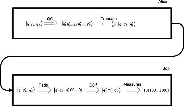
Figure 10.5. A quantum compression scheme.

i.e., the likelihood that the original message will be perfectly retrieved after the receiver pads the compressed message, applies the inverse maps and finally measures it.

In plain words, a quantum compressor is a unitary (and therefore invertible) map such that most transformed messages have only k significant qubits, i.e., they lie almost completely within a k-dimensional subspace known as the typical subspace.

If Alice owns such a quantum compressor, she and Bob have a well-defined strategy to compress qubit streams (shown in Figure 10.5):

Step 1. She applies the compressor to her message. The result’s amplitudes can be safely set to zero except for the ones corresponding to the typical subspace. After a rearrangement, the amplitudes have been listed so that the first k belong to the subspace and the other n− k are the ones that are negligible and can be thus set to zero.

Step 2. Alice truncates her message to the significant k qubits, and sends it to Bob.

Step 3. Bob appends to the received message the missing zeros (padding step), and

Step 4. Bob changes back the padded message to the original basis.

Step 5. He then measures the message and reads it.

How and where is Alice to find her quantum processor? As before, to build up our intuition, we are going to analyze a concrete example. Let us go back to Example 10.2.2 and use the same setup. Alice’s quantum alphabet consists of the two vectors and , which she sends with frequency and , respectively. A message of length n will look like

where

Suppose that Alice, before sending the message, changes basis. Instead of the canonical basis, she chooses the eigenvector basis of the density matrix, i.e., the vectors and that we explicitly computed in Example 10.2.4.

Alice’s message can be described in this basis as

What is the benefit of this change of basis? As a vector, the message is still a point in , and so its length has not changed. However, something quite interesting is happening here. We are going to find out that quite a few of the c_i’s are indeed so small that they can be discarded. Let us calculate first the projections of and along the eigenvectors e₁ and e₂:

We have just discovered that the projection of either or along is smaller than their components along .

Using the projections of Equation (10.71), we can now calculate the components c_i in the eigenbasis decomposition of a generic message. For instance, the message equal to has the component along

Exercise 10.3.4 Assume the same setup as the previous one, and consider the message . What is the value of the component along ?

Many of the coefficients c_i are dispensable, as we anticipated (see Figure 10.6.)

The significant coefficients turn out to be the ones that are associated with typical sequences of eigenvectors, i.e., sequences whose relative proportions of and are consistent with their probabilities, calculated in Equations (10.54) and (10.55). The set of all these typical sequences spans a subspace of , the typical subspace we were looking for. Its dimension is given by 2^N×H(S), where H(S) is the von Neumann entropy of the source. Alice and Bob now have a strategy for compressing and decompressing qubit sequences, following the recipe sketched earlier in Steps 1–5.

We have just shown a specific example. However, what Alice found out can be generalized and formally proved, leading to the quantum analog of Shannon’s coding theorem, due to Benjamin Schumacher (1995b).

Theorem 10.3.2 (Schumacher’s Quantum Coding Theorem.) A qubit stream of length n emitted from a given quantum source QS of known density can be compressed on average to a qubit stream of length n× H(QS), where H(QS) is the von Neumann entropy of the source. The fidelity approaches one as n goes to infinity.

Figure 10.6. Source as in Example 10.2.2: , , n = 12, H(S)=0.54999.

Note: In a sense, the bound n× H(QS) represents the best we can do with quantum sources. This theorem is particularly exciting in light of what we have seen at the end of the last section, namely, that von Neumann entropy can be lower than classical entropy. This means that, at least in principle, quantum compression schemes can be designed that compress quantum information in a tighter way than classical information can be in the classical world.

However, this magic comes at a price: whereas in the classical arena one can create purely lossless data compression schemes, this is not necessarily so in the quantum domain. Indeed, if Alice chooses her quantum alphabet as a set of nonorthogonal states, there is no measurement on Bob’s side whose eigenvectors are precisely Alice’s “quantum letters.” This means that perfect reconstruction of the message cannot be ensured. There is a trade-off here: the quantum world is definitely more spacious than our own macroscopic world, thereby allowing for new compression schemes, but at the same time it is also fuzzy, carrying an unavoidable element of intrinsic indeterminacy that cannot be ignored.

Programming Drill 10.3.3 Write a program that lets the user enter two qubits and their corresponding probabilities. Then calculate the density matrix, diagonalize it, and store the corresponding eigenbasis. The user will then enter a quantum message. The program will write the message in the eigenbasis and return the truncated part belonging to the typical subspace.

10.4 ERROR-CORRECTING CODES

There is yet another aspect of information theory that cannot be ignored. Information is always sent or stored through some physical medium. In either case, random errors may happen: our valuable data can degrade over time.

Errors occur with classical data, but the problem is even more serious in the quantum domain: as we shall see in Chapter 11, a new phenomenon known as decoherence makes this issue absolutely critical for the very existence of a reliable quantum computer.

As a way to mitigate this unpleasant state of affairs, information theory researchers have developed a large variety of techniques to detect errors, as well as to correct them. In this last section we briefly showcase one of these techniques, both in its classical version and in its quantum version.

As we have just said, our enemy here is random errors. By their very definition, they are unpredictable. However, frequently we can anticipate which types of errors our physical devices are subjected to. This is important: by means of this knowledge we can often elaborate adequate defense strategies.

Suppose you send a single bit, and you expect a bit flip error 25% of the time. What would you do? A valid trick is simply repetition. Let us thus introduce an elementary repetition code:

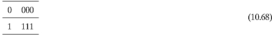
We have simply repeated a bit three times. One can decode the triplet by majority law: if at least two of the qubits are zeros, it is zero; else, it is one.

Exercise 10.4.1 What is the probability of incorrectly decoding one bit?

Now, let us move on to qubit messages. Qubits are less “rigid” than bits, so new types of errors can occur: for instance, aside qubit-flips

signs can be flipped too:

Exercise 10.4.2 Go back to Chapter 5 and review the Block sphere representation of qubits. What is the geometric interpretation of sign flip?

To be sure, when dealing with qubits other types of errors can occur, not just “jumpy” errors (i.e., discrete ones). For instance, either α or β could change by a small amount. For example, α might have a change of phase by 15º. For the sake of simplicity though, we shall only envision bit and sign flips.

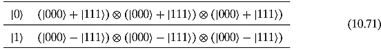
If we are looking for the quantum analog of the repetition code given in Equation (10.68), we must make sure that we can detect both types of errors. There is a code that does the job, due to Peter W. Shor (1995), known as the 9-qubit code¹⁰:

Why nine qubits? 3 × 3 = 9: by employing the majority rule twice, once for qubit flip and once for sign, we can correct both.

Exercise 10.4.3 Suppose that a sign flip occurs 25% of the times, and a single qubit flip 10% of the times. Also suppose that these two errors are independent of each other. What is the likelihood that we incorrectly decode the original qubit?

We have barely scraped the tip of an iceberg. Quantum error-correction is a flourishing area of quantum computing, and a number of interesting results have already emerged. If, as we hope, this small section has whetted your appetite, you can look into the references and continue your journey beyond the basics.

 

---

References: The first formulation of the basic laws of information theory is contained in the seminal (and readable!) paper “The mathematical theory of communication” written by Claude Shannon (Shannon, 1948). This paper is freely available online. A good reference for information theory and Shannon’s theorem is Ash (1990).

Huffman’s algorithm can be found, e.g., on pages 385–393 of Corman et al. (2001).

An excellent all-round reference on data compression is the text by Sayood (2005). For Schumacher’s theorem, take a look at the PowerPoint presentation by Nielsen.

Finally, Knill et al. (2002) is a panoramic survey of quantum error-correction.

¹ After all, this is just common sense. Would you bother reading a daily newspaper if you knew its content beforehand?

² The calculus savvy reader will promptly recognize the soundness of this convention: the limit of the function y = x log₂(x) is zero as x approaches zero. There is another more philosophical motivation: if a symbol is never sent, its contribution to the calculation of entropy should be zero.

³ The origin of the density operator lies in statistical quantum mechanics. The formalism that we have presented thus far works well if we assume that the quantum system is in a well-defined state. Now, when studying large ensembles of quantum particles, the most we can assume is that we know the probability distribution of the quantum states of the individual particles, i.e., we know that a randomly selected particle will be in state with probability p₁, etc.

⁴ Most texts introduce von Neumann entropy using the so-called Trace operator, and then recover our expression by means of diagonalization. We have sacrificed mathematical elegance for the sake of simplicity, and also because for the present purposes the explicit formula in terms of the eigenvalues is quite handy.

⁵ The difference between entropy in classical and quantum domains becomes even sharper when we consider composite sources. There entanglement creates a new type of order that is reflected by the global entropy of the system. If you want to know more about this phenomenon, go to Appendix E at the end of the book.

⁶ There are several notions of similarity used by the data compression community, depending on the particular needs one may have. Most are actually distances, meaning that they satisfy the triangular inequality, besides the two conditions mentioned here.

⁷ The extremely popular JPEG and MPEG formats, for images and videos, respectively, are two popular examples of lossy compression algorithms.

⁸ ZIP is a widely popular application based on the so-called Lempel–Ziv lossless compression algorithm, generally used to compress text files.

⁹ Huffman’s algorithm is actually optimal, i.e., it reaches Shannon’s bound, but only for special pdfs.

¹⁰ 9-qubit code is the first known quantum code.