In the application of probability theory a number of models arise time and time again. In many, diverse, real situations, engineers will often make assumptions about their physical problems which lead to analogous descriptions and hence to mathematically identical forms of the model. Only the numbers, for example, the values of the parameters of a model, and their interpretations differ from application to application. The random variables of interest in these situations have distributions which can be derived and studied independently of the specific application. These distributions have become so common that they have been given proper names and have been tabulated to facilitate their use.
The familiarity of these distributions in fact leads to their frequent adoption simply for reasons of computational expediency. Even though there may exist no argument (no model of the underlying physical mechanism) suggesting that a particular distribution is appropriate, it is often convenient to have a simple mathematical function to describe a variable. The distributions studied in this chapter are the ones most commonly adopted for this empirical use by the engineer. This is simply because they are well known, well tabulated, and easily worked with. In such situations the choice among common distributions is usually based on a comparison between the shape of a histogram of data and the shape of a PDF or PMF of the mathematical distribution. Examples will appear in this chapter, and the technique of comparison will be more fully discussed in Sec. 4.5. †
Such an empirical path is often the only one available to the engineer, but it should be remembered that in these cases the subsequent conclusions, being based on the adopted distribution, are usually dependent to a greater or lesser degree upon its properties. In order to make the conclusions as accurate and as useful as possible, and in order to justify, when necessary, extrapolation beyond available data, it is preferable that the choice of distribution be based whenever possible on an understanding of how the physical situation might have given rise to the distribution. For this reason this chapter is written to give the reader not simply a catalog of common distributions but rather an understanding of at least one mechanism by which each distribution might arise. To the engineer, the existence of such mechanisms, which may describe a physical situation of interest to him, is fundamentally a far more important reason for gaining familiarity with a particular common distribution than, say, the fact that it is a good mathematical approximation of some other distribution, or that it is widely tabulated.
From the pedagogical point of view this chapter has the additional purpose of reinforcing all the basic theory presented in Chap. 2. After the statement of the underlying mechanism, the derivation of the various distributions involved is only an application of those basic principles. In particular, derived distribution techniques will be applied frequently in this chapter.
Perhaps the single most common basic situation is that where the outcomes of experiments can be separated into two exclusive categories— for example, satisfactory or not, high or low, too fast or not, within specifications or not, etc. The following distributions arise from random variables of interest in this situation.
We are interested in the simplest kind of experiment, one where the outcomes can be called either a “success” or a “failure”; that is, only two (mutually exclusive, collectively exhaustive) events are possible outcomes. Examples include testing a material specimen to see if it meets specifications, observing a vehicle at an intersection to see if it makes a left turn or not, or attempting to load a member to its predicted ultimate capacity and recording its ability or lack of ability to carry the load.
Although at the moment it may hardly seem necessary, one can define a random variable on the experiment so that the variable X takes on one of two numbers—one associated with success, the other with failure. The value of this approach will be demonstrated later. We define, then, the “Bernoulli” random variable X and assign it values. For example,
The choice of values 1 and 0 is arbitrary but useful. Clearly, the PMF of X is simply
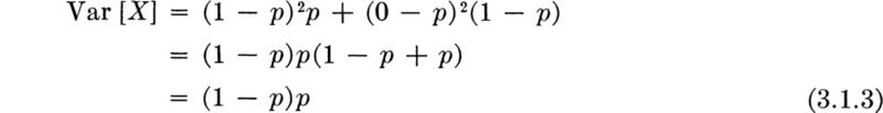
where p is the probability of success. The random variable has mean
and variance
As mentioned, another choice of values other than 0,1 might have been made, but this particular choice yields a random variable with an expectation equal to the probability of success p.
Thus, if one has a large stock of items, say high-strength bolts, and he proposes to select and inspect one to determine whether it meets specifications, the mean value of the Bernoulli random variable in such an experiment (with a “success” defined as finding an unsatisfactory bolt) is p, the proportion of defective bolts, † This direct correspondence between mX and p will prove useful when in Chap. 4 we discuss methods for estimating the mean value of random variables. Notice that the variance of X is a maximum when p is ½.
A sequence of simple Bernoulli experiments, when the outcomes of the experiments are mutually independent and when the probability of success remains unchanged, are called Bernoulli trials. One might be interested, for example, in observing five successive cars, each of which turns left with probability p; under the assumption that one driver’s decision to turn is not affected by the actions of the other four drivers, the set of five cars’ turning behaviors represents a sequence of Bernoulli trials. From a batch of concrete one extracts three test cylinders, each with probability p of failing at a stress below the specified strength; these represent Bernoulli trials if the conditional probability that any one will fail remains unchanged given that any of the others has failed. In each of a sequence of 30 years, the occurrence or not of a flood greater than the capacity of a spillway represents a sequence of 30 Bernoulli trials if maximum annual flood magnitudes are independent and if the probability p of an occurrence in any year remains unchanged throughout the 30 years, †
We shall be interested in determining the distributions of various random variables related to the Bernoulli trials mechanism.
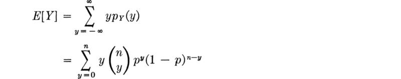
Distribution Let us determine the distribution of the total number of successes in n Bernoulli trials, each with probability of success p. Call this random number of successes Y. Consider first a simple case, n = 3. There will be no successes (that is, Y = 0) in three trials only if all trials lead to failures. This event has probability
![]()
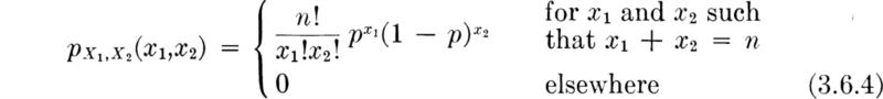
Any of the following sequences of successes 1 and failures 0 will lead to a total of one success in three trials:

Each sequence is an event with probability of occurrence p(l – p)2. Therefore the event Y = 1 has probability 3p(1– p)2, since the sequences are mutually exclusive events. Similarly, the mutually exclusive sequences

each occuring with probability p2(l – p), lead to Y = 2. Hence
![]()
Similarly, P[Y = 3] = p3, since only the sequence 1, 1, 1 corresponds to Y = 3. In concise notation,

where  indicates the binomial coefficient:

This coefficient is equal to the number of ways that exactly y successes can be found in a sequence of three trials. (Recall that 0! = 1, by definition.)
If the probability that a contractor’s bid will be low is ½ on each of three independent jobs, the probability distribution of Y, the number of successful bids, is
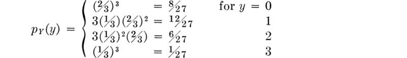
Contrary to some popular beliefs, it is not certain that the contractor will get a job; the likelihood is almost ⅓ that he will get no job at all!
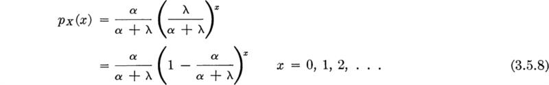
In general, if there are n Bernoulli trials, the PMF of the total number of successes Y is given by
It is clear that the parameter n must be integer and the parameter p
must be 0 ≤ p ≤ 1. The binomial coefficient
is the number of ways a sequence of n trials can contain exactly y successes Parzen [I960].
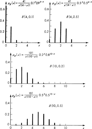
A number of examples of this, the “binomial distribution,’ are plotted in Fig. 3.1.1. The shape depends radically on the values of the parameters n and p. Notice the use of the notation B(n,p) to indicate a binomial distribution with parameters n and p; for example, the random variable Y in the bidding example above is B(3,⅓).
Fig. 3.1.1 Binomial distribution B(n,p).
Formally, the CDF of the binomial distribution is
Thus in the bidding example, the probability that the contractor will receive two or fewer bids is
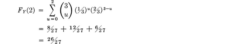
Or, more easily,
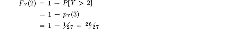
It is often the case that the probabilities of complementary events are more easily computed than those of the events themselves. As another example, the probability that the contractor gets at least one bid is

Moments The mean and variance of a binomial random variable Y are easily determined, and the exercise permits us to demonstrate some of the techniques of dealing with sums which many readers find unfamiliar. Thus,
Since the first term is zero, it can be dropped. The y cancels a term in y!:

Bringing np in front of the sum,

Letting u = y – 1,

Notice now that the sum is over all the elements of a B(n – 1, p) mass function and hence equals 1, yielding
This is an example of a most common method of approach in probability problems, namely, manipulating integrals and sums into integrals and sums over recognizable PDF or PMF’s, which are known to equal unity. In a similar manner, we can find

or
Y as a sum Notice that the total number of successes in n trials Y, can be interpreted as the sum
![]()
of n independent identically distributed Bernoulli random variables; thus Xi = 1 if there is a success on the ith trial, and Xi = 0 if there is a failure. As such, the results above could have been more easily obtained as
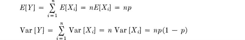
using Eqs. (3.1.2) and (3.1.3). The techniques of derived distributions (Sec. 2.3) could also have been used to find the distribution of Y from those of Xi The interpretation of a binomial variable as the sum of Bernoulli variables also explains why the sum of two binomial random variables, B(n1,p) and B(n2,p), also has a binomial distribution, B(n1 + n2, p) as long as p remains constant. This fact is easily verified using the techniques of Sec. 2.3.
The binomial distribution is tabulated, † but its evaluation, which is time-consuming for large n, can frequently be carried out approximately using more readily available tables of the Poisson distribution (Sec. 3.2.1) or the normal distribution (Sec. 3.3.1); Prob. 3.18 explains these approximations. The latter approximation is justified in Sec. 3.3.1 in the light of the binomial random variable’s interpretation as the sum of n Bernoulli random variables.
Rather than asking the question, “How many successes will occur in a fixed number of repeated Bernoulli trials?” the engineer may alternatively be interested in the question, “At what trial will the first success occur?” For example, how many bolts will be tested before a defective one is encountered if the proportion defective is p? When will the first critical flood occur if the probability that it will occur in any year is p?
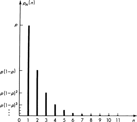
Geometric distribution Assuming independence of the trials and a constant value of p, the distribution of N, the number of trials to the first success, is easily found. The first success will occur on the nth trial if and only if (1) the first n – 1 are failures, which occurs with probability (1 – p)n–1 and (2) the nth trial is a success, which occurs with probability p, or
Notice that N may, conceptually at least, take on any value from one to infinity. ‡
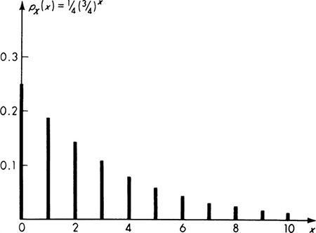
This distribution is called the geometric § distribution with parameter p. Symbolically we say that N is G(p). A plot of a geometric distribution appears in Fig. 3.1.2.
The cumulative distribution function of the geometric distribution is
Fig. 3.1.2 Geometric distribution G(p).
where use is made of the familiar formula for the sum of a geometric progression. This result could have been obtained directly by observing that the probability that N ≤ n is simply the probability that there is at least one occurrence in n trials, or
![]()
The geometric distribution also follows from a totally different mechanism (see Sec. 3.5.3).
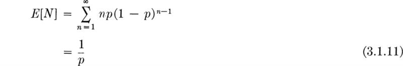
Moments of the geometric The first moment of a geometric random variable is found by substitution and a number of algebraic manipulations similar to those used in the binomial case. The reader can show that
In words, the average number of trials to the first occurrence is the reciprocal of the probability of occurrence on any one trial. For example, if the proportion of defective bolts is 0.1, on the average, 10 bolts would be tested before a defective would be found, assuming the conditions of independent Bernoulli trials hold.
The variance of N can easily be shown to be
Negative binomial distribution We have just determined the answer to the question, “On which trial will the first success occur?” Next consider the more general question, “On which trial will the kth success occur?” We are dealing now with a random variable, say Wk, which is the sum of random variables N1N2, . . ., Nk, where Ni is the number of trials between the (i – l)th and ith successes. Thus
![]()
Because of the assumed independence of the Bernoulli trials, it is clear that the Ni: (i = 1,2, . . . k) are mutually independent random variables, each with a common geometric distribution with parameter p. As a result of this observation, we can obtain partial information about Wk, namely, its moments, very easily. The mean and variance of Wk can be written down immediately as
The distribution of W can be found using the methods discussed in Sec. 2.3. For example, for k = 2,
![]()
Writing Eq. (2.3.43) for the discrete case, we have

which states that the probability that W2 = w is the probability that N1= n and N2= w – n, summed over all values of n up to w. Notice that when n = w in the sum, we get ![]() , which is zero; hence
, which is zero; hence
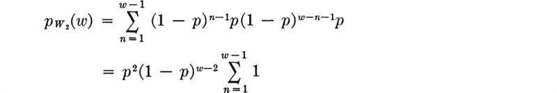
or, simply,
This result could have been arrived at directly by arguing that the second success will be achieved at the wth trial only if there are w – 2 failures, a success on the wth trial, and one success in any one of the w – 1 preceding trials.
With this result for W2, one could find the distribution of W3, knowing W3 = W2+ N3. In turn the distribution for any k could be arrived at. If this exercise is carried out, a pattern emerges immediately, and one can conclude that
The result is reasonable if one argues that the kth success occurs on wth trial only if there are exactly k – 1 successes in the preceding w – 1 trials and there is a success on the wth trial. The probability of exactly k – 1 successes in w – 1 trials we know from our study of binomial random variables to be 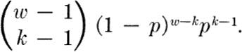
This distribution is known as the Pascal, or negative binomial, distribution with parameters k and p, denoted here NB(k,p).† It has been widely used in studies of accidents, ‡ cosmic rays, learning processes, and exposure to diseases. It should not be surprising, owing to its possible interpretation as the number of trials to the (k1 + k2)th event, that a random variable which is the sum of a NB(k1,p) and a NB(k2,p) pair of (independent) random variables is itself negatively binomially distributed, NB(k1 + k2, p).
Illustration: Turn lanes If a left-turn lane at a traffic light has a capacity of three cars, what is the probability that the lane will not be sufficiently large to hold all the drivers who want to turn left in a string of six cars delayed by a red signal? In the mean, 30 percent of all cars want to turn left. The desired probability is simply the probability that the number of trials to the fourth success (left-turning car) is less than 6. Letting WA equal that number, W4 has a negative binomial distribution. Therefore,
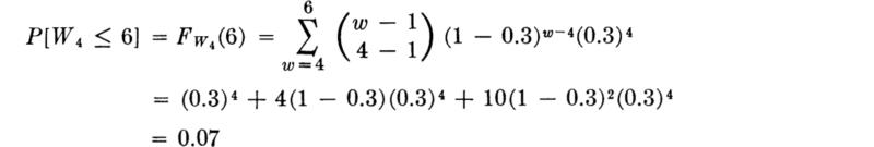
Alternatively, one could have deduced this answer by asking for the probability of four, five, or six successes in six Beroulli trials and used the PMF of the appropriate binomial random variable.
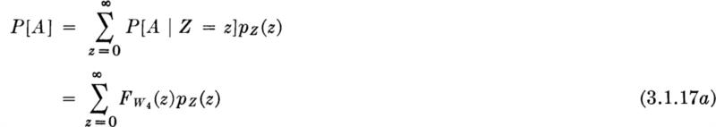
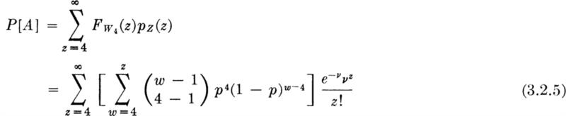
A more realistic question might be, “What is the probability that the left-turn lane capacity will be insufficient when the number of red-signal-delayed cars is unspecified?” This number is itself a random variable, say Z, with a probability mass function, pz(z), z = 0, 1, 2, .... Then the probability of the event A, that the lane is inadequate, is found by considering all possible values of Z:
or, since Fw4(z)= 0 for z < 4,
A logical choice for the mass function of Z will be considered in the following section, Sec. 3.2.1.
Illustration: Design values and return periods In the design of civil engineering systems which must withstand the effects of rare events such as large floods or high winds, it is necessary to consider the risks involved for any particular choice of design capacity. Given a design, the engineer can usually estimate the largest magnitude of the rare event which the design can withstand, e.g., the maximum flow possible through a spillway or the maximum wind velocity which a structure can resist. The engineer then seeks (from past data, say) an estimate of the probability p that in a given time period, usually a year, this critical magnitude will be exceeded.
If, as is commonly assumed, the magnitude of the maximum annual flow rates in a river or the maximum annual wind velocities are independent, and if p remains constant from year to year, then the successive years represent independent Bernoulli trials. A magnitude greater than the critical value is denoted a success. With the knowledge of the distributions in this section the engineer is now in a position to answer a number of critical questions.
Let us assume, for example, that p = 0.02; that is, there is 1 chance in 50 that a flood greater than the critical value will occur in any particular year. What is the probability that at least one large flood will take place during. the 30-year economic lifetime of a proposed flood-control system? Let X equal the number of large floods in 30 years. Then X is B(30,0.02), and
![]()
Using the familiar binomial theorem,
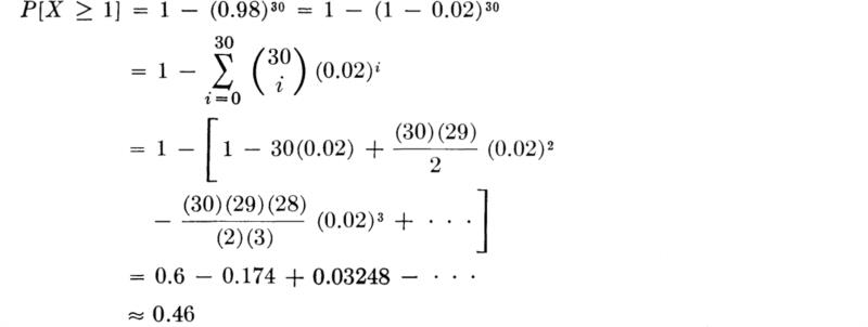
If this risk of at least one critical flood is considered too great relative to the consequences, the engineer might increase the design capacity such that the magnitude of the critical flood would only be exceeded with probability 0.01 in any one year. Then X is B(30,0.01), and
![]()
The engineer seeks, of course, to weigh increased initial cost of the system versus the decreased risk of incurring the damage associated with a failure of the system to contain the largest flood.
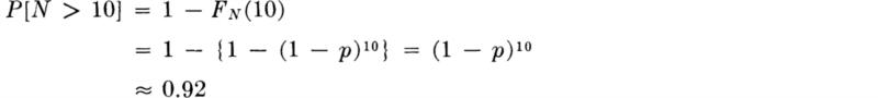
The number of years N to the first occurrence of the critical flood is a random variable with a geometric distribution, G(0.01), in the latter case. The probability that it is greater than 10 years is
What is the probability that N > 30? Clearly it is just equal to the probability that there are no floods in 30 years, i.e., that X = 0, where X is B(30,0.01). Here, using a previous result,

Average Return Periods The expected value of N is simply

This is the average number of trials (years) to the first flood of magnitude greater than the critical flood. In civil engineering this is referred to as the average return period or simply the return period. The critical magnitude is often referred to as the “mN-year flood,” here the “100-year flood.” The term is somewhat unfortunate, since its use has led the layman to conclude that there will be 100 years between such floods when in fact the probability of such a flood in any year remains 0.01 independently of the occurrence of such a flood in the previous or a recent year (at least according to the engineer’s model).
The probability that there will be no floods greater than the m-year flood in m years is, since X is then B[m,l/m],
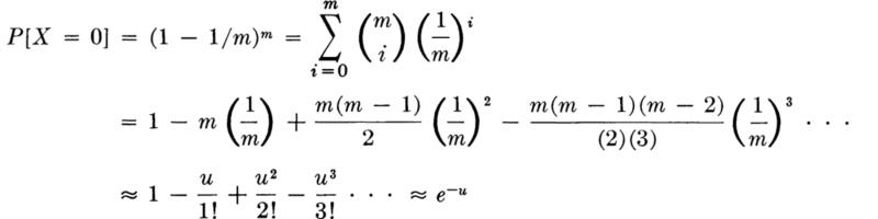
where u = m(l/m) = 1; hence, for large m,
![]()
That is, the likelihood that one or more m-year events will occur in m years is approximately 1 – e–1= 0.632. Thus a system “designed for the m-year flood” will be inadequate with a probability of about 2/3 at least once during a period of m years.
Cost Optimization What is the optimum design to minimize total expected cost? Assume that the cost c associated with a system failure is independent of the flood magnitude, and that, in the range of designs of interest, the cost is a constant I plus an incremental cost whose logarithm is proportional to the mean return period mN of the design demand, † For an economic design life of 30 years,

Since the cost of failure is cX,
![]()
Assume that the system itself remains in use with an unaltered capacity after any failure. Then, if X is the number of failures in 30 years, it is distributed
B(30, 1/mN) (assuming no more than one failure per year). The mean of X is 30/mN. The expected cost, given a value of mN, is
![]()
The design flood magnitude ![]() , which minimizes this expected total cost, is found by setting the derivative of total cost equal to zero:
, which minimizes this expected total cost, is found by setting the derivative of total cost equal to zero:
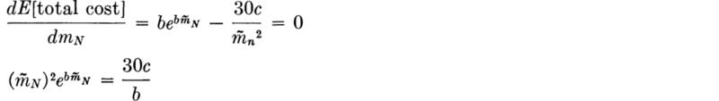
This equation can be solved by trial and error for given values of b and c. For example, for b = 0.1 year-1 and c = $200,000, ![]() years. Thus the designer should provide a system with a capacity sufficient to withstand the demand which is exceeded with probability 1/90 = 0.011 in any year. In Sec. 3.3, we will encounter distributions commonly used to describe annual maximum floods from which such design magnitudes could be easily obtained, once the design return period is fixed.
years. Thus the designer should provide a system with a capacity sufficient to withstand the demand which is exceeded with probability 1/90 = 0.011 in any year. In Sec. 3.3, we will encounter distributions commonly used to describe annual maximum floods from which such design magnitudes could be easily obtained, once the design return period is fixed.
The basic model discussed here is that of Bernoulli trials. They are a sequence of independent experiments, the outcome of any one of which can be classified as either success or failure (or, numerically, 0 or 1). The probability of success p remains constant from trial to trial.
If this model holds, then:
1. Y, the total number of successes in n trials, has a binomial distribution:

with mean np and variance np(1 – p).
2. N, the trial number at which the first success occurs, has a geometricdistribution:
![]()
with mean 1/p and variance (1 – p)/p2. The former is called the mean return period.
3. Wk, the trial number at which the kth success will occur, has a negative binomial distribution:

with mean k/p and variance k (l – p)/p2.
In many situations it is not possible to identify individual discrete trials at which events (or successes) might occur, but it is known that the number of such trials is many. The models in this section arise out of consideration of situations where the number of possible trials is infinitely large. Examples include situations where events can occur at any instant over an interval of time or at any location along the length of a line or on the area of a surface.
A derivation of the distribution Suppose that a traffic engineer is interested in the total number of vehicles which arrive at a specific location in a fixed interval of time, t sec long. If he knows that the probability of a vehicle occurring in any second is a small number p, (and if he assumes that the probability of two or more vehicles in any one second is negligible), then the total number of vehicles X in the n = t (assumed) independent trials is binomial, B(n,p):

Consider what happens as the engineer takes smaller and smaller time durations to represent the individual trials. The number of trials n increases and the probability p of success on any one trial decreases, but the expected number events in the total interval must remain constant at pn. Call this constant ν and consider the PMF of X in the limit as the trial duration shrinks to zero, such that

Substituting for p = ν/n in the PMF of X and rearranging,
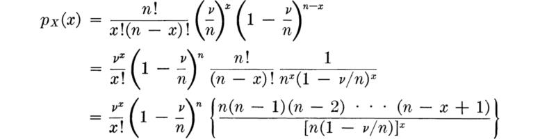
The term in braces has x terms in the numerator and x terms in the denominator. For large n each of these terms is very nearly equal to n; hence in the limit, as n goes to infinity, the term in braces is simply nx/nx or 1. The term (1 – ν/n)n is known to equal e–ν in the limit. Hence the PMF of X is
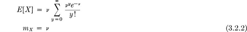
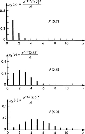
Moments This extremely useful distribution is known as the Poisson distribution, denoted here P(ν). Notice it contains but a single parameter ν, compared with the two required for the binomial distribution, B(n,p). Its mean and variance are both equal to this parameter. Following the same steps used to find the mean of the binomial distribution,
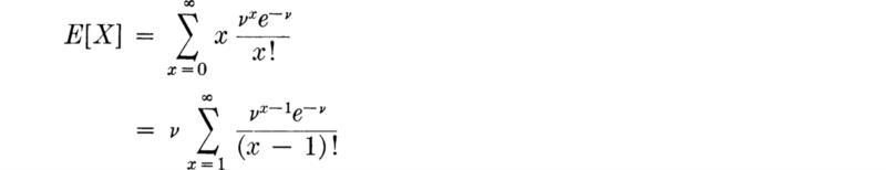
Letting y = x – 1,
since the sum is now simply the sum over a Poisson PMF. A similar calculation shows that also
Plots of Poisson distributions are displayed in Fig. 3.2.1. † Notice the fading of skew as ν increases.
Also, consideration of the derivation should make it clear that the sum of two Poisson random variables with parameters vx and v2 must again be a Poisson random variable with parameters ν= ν1 + ν2- (How might this fact be verified?) Distributions with the peculiar and valuable property that the sum of independent random variables with the distribution has the same distribution are said to be “regenerative.” The binomial and negative binomial distributions are, recall, regenerative only on the condition that the parameter p is the same for all the distributions.
Poisson process It is clear from the derivation that if a time interval of a different duration, say 2t, is of interest, then the number of trials at any stage in the limit would be twice as great and the parameter of the resulting Poisson distribution would be 2ν. In such cases, the parameter of the Poisson distribution can be written advantageously as λt rather than ν:
Fig. 3.2.1 Poisson distribution P(ν).
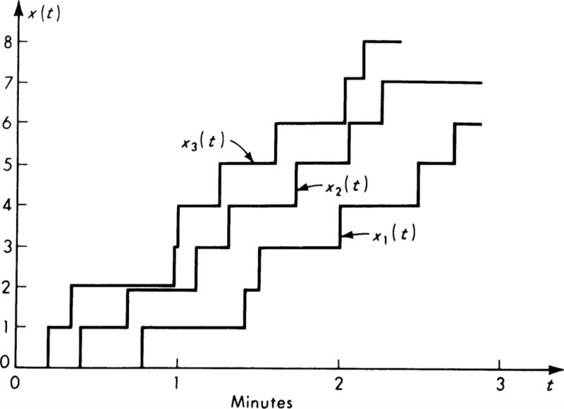
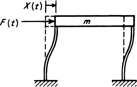
This form of the Poisson distribution is suggestive of its association with the Poisson process. A stochastic process is a random function of time (usually). In this case we are interested in a stochastic process X(t), whose value at any time t is the (random) number of arrivals or incidents which have occurred since time t = 0. Just as samples of a random variable X are numbers, x1, x2, . . ., so observations of a random process X(t) are sample functions of time, x1(t), x2(t), . . ., as shown in Fig. 3.2.2.
Fig. 3.2.2 Sample functions of a Poisson process X(t).
The samples shown there are of a Poisson process which is counting the number of vehicle arrivals versus time. Other examples of stochastic processes include wave forces versus time, total accumulated rainfall versus time, and strength of soil versus depth. We will encounter other cases of stochastic processes in Secs. 3.6 and 3.7 and in Chap. 6.
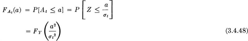
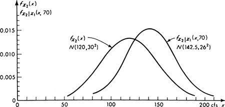
At any fixed value of the (time) parameter t, say t = t0, the value X(t0) of a stochastic process is a simple random variable, with an appropriate distribution ![]() which has an appropriate mean
which has an appropriate mean ![]() variance
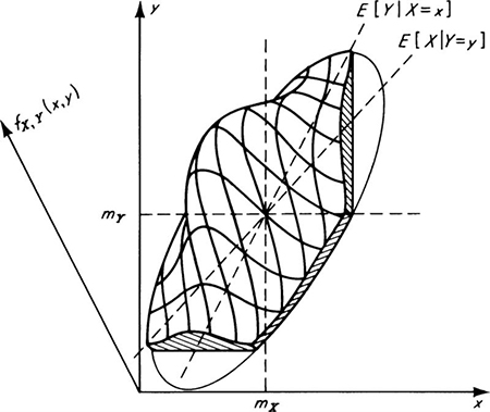
variance ![]() etc.† In general, this distribution, mean, and variance are functions of time. In addition, the joint behavior of two (or more) values, say X(t0) and X(t1), of a stochastic process is governed by a joint probability law. Typically one might be interested in studying the conditional distribution of a future value X(t1), given an observation at the present time X(t0), in order to “predict” that future value (e.g., see Sec. 3.6.2).
etc.† In general, this distribution, mean, and variance are functions of time. In addition, the joint behavior of two (or more) values, say X(t0) and X(t1), of a stochastic process is governed by a joint probability law. Typically one might be interested in studying the conditional distribution of a future value X(t1), given an observation at the present time X(t0), in order to “predict” that future value (e.g., see Sec. 3.6.2).
An elementary result of the study of stochastic processes‡ is that the distribution of the random variable X(t0) is the Poisson distribution with parameter λt0 if the stochastic process X(t) is a Poisson process with parameter λ. To be a Poisson process, the underlying physical mechanism generating the arrivals or incidents must satisfy the following important assumptions:
1. Stationarity. The probability of an incident in a short interval of time t to t + h is approximately λh, for any t.
2. Nonmultiplicity. The probability of two or more events in a short interval of time is negligible compared to λh (i.e., it is of smaller order than λh).
3. Independence. The number of incidents in any interval of time is independent of the number in any other (nonoverlapping) interval of time.
The close analogy to the assumptions underlying discrete Bernoulli trials (Sec. 3.1) is evident. Therefore, the observed convergence of the binomial distribution to the Poisson distribution is to be expected.
In short, if we are observing a Poisson process, the distribution of X(t) at any t is the Poisson distribution [Eq. (3.2.4)], with mean mX(t)=λt [from Eq. (3.2.2)]. Therefore, the parameter λ is usually referred to as the average rate (of arrival) of the Poisson process.
The basic mechanism from which the Poisson process arises, namely, independent incidents occurring along a continuous (time) axis with a constant average rate of occurrence, suggests why it is often referred to as the “model of random events” (or random arrivals). It has been successfully employed to describe such diverse problems as the occurrences of storms (Borgman [1963]), major floods (Shane and Lynn [1964]), overloads on structures (Freudenthal, Garrelts, and Shinozuka [1966]), and, distributed in space rather than time, flaws in materials and particles of aggregate in surrounding matrices of material,† It is also widely employed in other fields of engineering to describe the arrival of telephone calls at a central exchange and the demands upon service facilities.
The Poisson process is often used by traffic engineers to model the flow of vehicles past a point when traffic is freely flowing and not dense (e.g., Greenshields and Weida [1952], Haight [1963]). For this reason the Poisson distribution describes well the number of vehicles which arrive at an intersection during a given time interval, say a cycle of a traffic light. The distribution logically might have been used in the illustrations dealing with traffic lights in Secs. 2.3 and 3.1.
Illustration: Left-turn lane and the model of random selection If, in the illustration in Sec. 3.1.2 involving left-turning cars at a traffic light, the number Z of cars arriving during one cycle is Poisson-distributed with parameter ν = 6, the
probability that less than four cars will arrive is
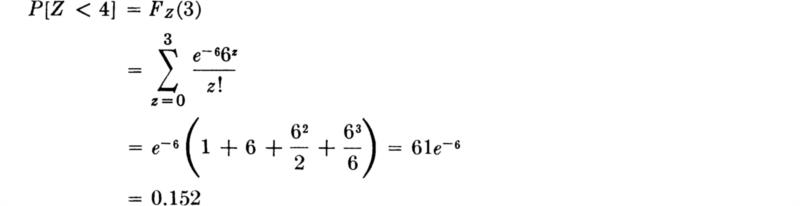
If this event occurs, there is no chance that the left-turn lane capacity will be exceeded. The probability of the event A, that the lane will be inadequate on any cycle (assuming there are no cars remaining from a previous cycle), is given in Eq. (3.1.17b):
where p is the proportion of cars turning left. This result could be evaluated as it stands for any values of p and v, but it is more informative to reason to another, simpler form.
If the probability is p that any particular car will turn left, then we can consider directly the arrival only of those cars which desire to turn left. Returning to the derivation of the Poisson distribution from the binomial, one can see that, since such left-turning cars arrive with a probability † p times the probability that any car arrives, the number X of these left-turning cars is also Poisson-distributed, but with parameter pv.‡ Hence the probability that the left-turn lane is inadequate is simply the probability that X is greater than or equal to four, or§:

For ν = 6 and p = 0.3, pν = 1.8 and
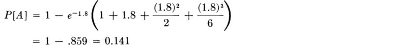
If this number is considered by the engineer to be too large, he might consider increasing the capacity of the lane in order to reduce the likelihood of inadequate performance.
It is important to realize the generality of the result used here. The implication is that if a random variable Z is Poisson-distributed, then so too is the random variable X, which is derived by (independently) selecting only with probability p each of the incidents counted by Z; that is if Z is P(ν), then X is P(pν). More formally, the distribution of X is found as

The conditional term is simply the probability of observing x successes in z Bernoulli trials; thus
which, upon changing the variable to u = z – x, reduces to
Examples of application of this result might include X being the number of hurricane-caused floods greater than critical magnitude when Z is the total number of hurricane arrivals, or X being the number of vehicles recorded by a defective counting device when Z is the total number of vehicles passing in a given interval. The latter example was encountered in Sec. 2.2.2 when the joint distribution of X and Z was investigated.
The traffic engineer observing a traffic stream is often concerned with the length of the time interval between vehicle arrivals at a point. If an interval is too short, for example, it will cause a car attempting to cross or merge with the traffic stream to remain stationary or to interrupt the stream. Let us seek the distribution for this time between arrivals under the conditions describing traffic flow used in the preceding section, namely, that the vehicles follow a Poisson arrival process with average arrival rate λ.
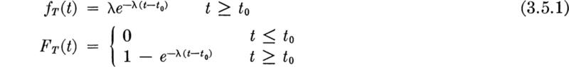
Distribution and moments If we denote by random variable T the time to the first arrival, then the probability that T exceeds some value t is equal to the probability that no events occur in that time interval of length t. The former probability is 1 – FT(t). The latter probability is px(0) the probability that a Poisson random variable X with parameter λt is zero. Substituting into Eq. (3.2.4),
![]()
Therefore,
while
This defines the “exponential” distribution which we shall denote EX(λ). It describes the time to the first occurrence of a Poisson event. Therefore it is a continuous analog of the geometric distribution [Eq. (3.1.3)]. But, owing to the stationarity and independence oroperties of the Poisson process, e–λt is the probability of no events in xny interval of time of length t, whether or not it begins at time 0. If we use the arrival time of the nth event as the beginning of the time interval, then e–λt is the probability that the time to the (n + 1)th event is greater than t. In short, the interarrival times of a Poisson process are independent and exponentially distributed.
The mean of the exponential distribution is
![]()
Letting u = λt,
Recall that in the previous section, λ was found to be the average number of events per unit time, while here 1/λ is revealed as the average time between arrivals.
In a similar manner,
Notice that the coefficient of variation of T is unity for any value of the parameter λ.
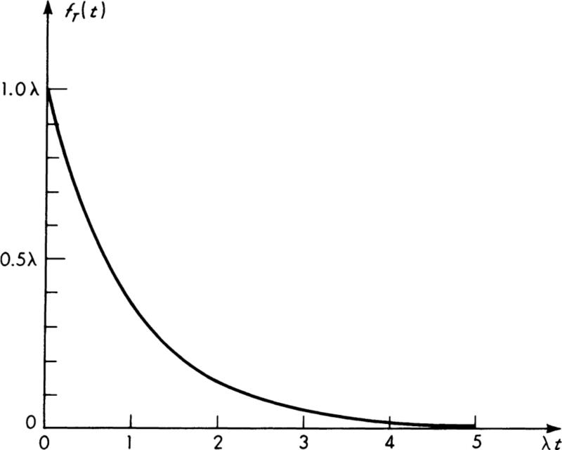
The exponential distribution is plotted in Fig. 3.2.3 as a function of λt, the ratio of t to the mean interarrival time. The distribution of
Fig. 3.2.3 Exponential distribution EX(λ).
the sum of two independent exponential random variables with different parameters α. and β was discussed in Sec. 2.3.2.
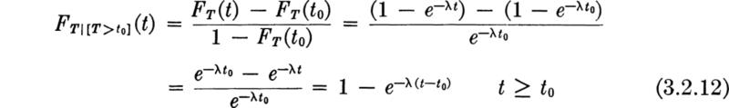
Memoryless property The Poisson process is often said to be “memory-less,” meaning that future behavior is independent of its present or past behavior. This memoryless character of the Poisson arrivals and of the exponential distribution is best understood by determining the conditional distribution of T given that T > t0, that is, the distribution of the time between arrivals given that no arrivals occurred before t0:

For t less than t0, the numerator is zero; for t ≥ t0 it is simply equal to P[t0 < T ≤t]. Thus
Or if time r is reckoned from t0, τ = t — t0,
In words, failure to observe an event up to t0 does not alter one’s prediction of the length of time (from t0) before an event will occur. The future is not influenced by the past if events are Poisson arrivals. An implication is that any choice of the time origin is satisfactory for the Poisson process.
Applications The very tractable exponential distribution is widely adopted in practice. The close association between the Poisson distribution and the exponential distribution, both arising out of a mechanism of events arriving independently and “at random” suggests that the exponential is applicable to the description of interarrival times (or distances, in the case of flaw distribution, for example) in those situations mentioned in Sec. 3.2.1 in which the number of events in a fixed interval is Poisson distributed. In addition, observed data is often suggestive of an exponential distribution even when the assumptions of a Poisson-arrivals mechanism may not seem wholly appropriate. Times between vehicle arrivals, for example, are influenced (for small values at least) by effects such as minimum spacings between vehicles and “platooning” of vehicles behind a slower vehicle, implying a lack of independence between event arrivals in two neighboring short intervals. Nonetheless, experience† has indicated that in many circumstances the adoption of the exponential distribution of vehicle interarrival times is reasonable. In studies of the lengths of the lifetimes in service of mechanical and electrical components, the analytical tractability of the exponential distribution has led to its wide adoption, even though gradual wearout of such components would suggest that the risk of failure in intervals of equal length would not be constant in time. This time dependence is, of course, in contradiction to the stationarity assumption in the Poisson process model, which predicts that the exponential distribution will describe interarrival times. In short, the exponential distribution, like many others we will encounter, is often adopted simply as a convenient representation of a phenomenon when no more than the shape of the observed data or the analytical tractability of the exponential function seem to suggest it.
Distribution and moments As in the case with discrete trials, it is also of interest to ask for the distribution of the time Xk to the kth arrival of a Poisson process. Now, the times between arrivals, Ti, i = 1,2, . . ., k, are independent and have exponential distributions with common parameter λ. Xk is the sum T1 + T2+ · · · + Tk. Its distribution follows from repeated application of the convolution integral, Eq. (2.3.43). † For any k = 1, 2, 3, . . . ,
We say X is gamma-distributed with parameters k and λ, G(k,λ)‡ if its density function has the form in Eq. (3.2.15). By integration or, more simply, by consideration of X as the sum of k independent exponentially distributed random variables, if X is G(k,λ), then
and
In fact, the gamma distribution is more broadly defined than is implied by its derivation as the distribution of the sum of k independently, identically distributed exponential random variables. More generally the parameter k need not be integer-valued § when the gamma distribution is written
the only restrictions being λ > 0 and k > 0. The gamma function Γ(k) (from which the distribution gets its name) is equal to (k – 1)! if k is an integer, but more generally is defined by the definite integral
The integral arises here as a constant needed to normalize the function to a proper density function. The gamma function is widely tabulated,
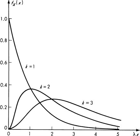
Fig. 3.2.4 Gamma distributions G(k,λ).
as is the “incomplete gamma function”:
which can be used to evaluate the cumulative distribution function Fx(x):†
The equations given above for the mean and variance of X hold for noninteger k as well.
The shape of the gamma density function, Fig. 3.2.4, indicates why it is widely used in engineering applications. Like observed data from many phenomena it is limited to positive values and is skewed to the right. Notice that λ can be interpreted as a scaling parameter and k as a shape parameter of the distribution. The skewness coefficient is
Owing to this shape and its convenient mathematical form (rather than to any belief that it arose from a fundamental, underlying mechanism where the time to the kth occurrence of some event was critical), the gamma distribution has been used by civil engineers to describe such varied phenomena as maximum stream flows (Markovic [1965]), the yield strength of reinforced concrete members (Tichy and Vorlicek [1965]), and the depth of monthly precipitation (Whitcomb [1940]).
In addition to its ability to describe observed data, the gamma distribution is, of course, important as the time to the occurrence of the kth [or the time between the nth and (n + k)th occurrence] in a Poisson process, † Applications include the time to the arrival of a fixed number of vehicles, and the time to the failure of a system designed to accept a fixed number of overloads before failing, when the vehicles and the overloads are Poisson arrivals. The sum of exponentials interpretation explains (at least for integer k) why the gamma is regenerative under fixed λ; that is, if X is G(k1,λ), Y is G(k2,λ), and Z = X + Y, then Z is G(k1+ k2, λ) if X and Y are independent. The result is true for noninteger k as well.
Illustration: Maximum flows Based on a histogram of data of maximum annual river flows in the Weldon River at Mill Grove, Missouri, for the years 1930 to 1960, the distribution was considered as a model by Markovic [1965]. The parameters were estimated ‡ as k = 1.727 and λ = 0.00672 (cfs)–1.
The mean is
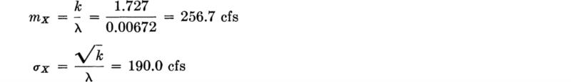
The probability that the maximum flow is less than 400 cfs in any year is (λ400 = 2.70):
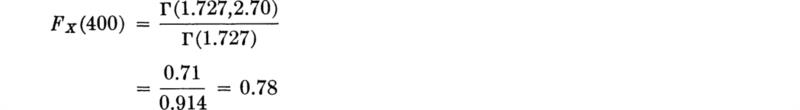
These values were taken from tables of the gamma function. In Sec. 3.4 more convenient tables will be introduced exploiting a simple relationship between the gamma and the widely tabulated “chi-square distribution.”
In a Poisson stochastic process incidents occur “at random” along a time (or other parameter) axis. If the conditions of stationarity, non-multiplicity, and independence of nonoverlapping intervals hold, then for an average arrival rate λ,
1. For any interval of time of length t, the number of events X which occur has a Poisson distribution with parameter ν = λt:

The mean and variance are both equal to ν.
2. The distribution of time T between incidents has an exponential distribution with parameter λ:
![]()
with mean 1/λ and variance 1/λ2.
3. The time Sk between k incidents has a gamma distribution:

with mean k/λ and variance k/λ2. The distribution is also defined for noninteger k when (k – 1)! should be replaced by Γ(k).
The single most important class of models is that in which the model arises as a limit to an argument about the relationship between the phenomenon of interest and its (many) “causes.” The uncertainty in a physical variable may be the result of the combined effects of many contributing causes, each difficult to isolate and observe. In several important situations, if we know the mechanism by which the individual causes affect the variable of interest, we can determine a model (or distribution) for the latter variable without studying in detail the individual effects. In particular, we need not know the distributions of the causes. Three important cases will be considered—that where the individual causes are additive, that where they are multiplicative, and that where their extremes are critical.
Convergence of the shape of the distribution of sums We shall introduce this case through an example. The total length of an item may be made up of the sum of the lengths of a number of similar individualparts. Examples are the total length of a line of cars in a queue, the total error in a long line surveyed in 100-ft increments, or the total time spent repeating a number of identical operations in a construction schedule.
Suppose, as a specific example, that the total length of several pieces is desired, and each has been measured on an accurate rule and recorded to the nearest even number of units (for example, 248 mm). It may be reasonable to assume that each “error,” that is, each difference between the recorded length and the true length, is in this case equally likely to lie anywhere between plus and minus one unit (e.g., the true length is between 247 and 249 mm).
Let us define a random variable:
Xi = the measurement error in the ith piece
Then by our argument this variable has a constant (or uniform, Sec. 3.4.1) density function

Consider first the total error in the combined length of two pieces, that is, the difference between the sum of their recorded lengths and the sum of their true lengths. Let

Assuming that the two measurement errors are unrelated, i.e., that X1 and X2 are independent random variables, we can determine the density function of Y2 using Eq. (2.3.43). The following result will be found:

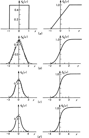
The distributions of Xi (or Y1) and Y2 are shown in Fig. 3.3.1.
The density function of Y3 = X1 + X2 + X3 is found in the same manner:
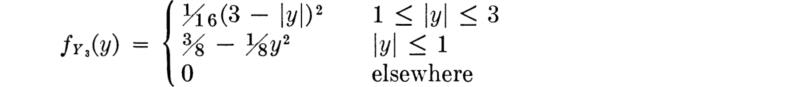
Similarly, we find too
These results are sketched in Fig. 3.3.1, along with the corresponding cumulative distribution functions. Note the scale changes.
Looking at the sequence of curves, it is evident that the distribution of the sum of a number of uniformly distributed random variables quickly takes on a bell-shaped form. By proper adjustment of the parameter c in each case,† a density function of the form
will closely approximate the density functions of the successive Yi. Such curves are shown in Fig. 3.3.1 as dotted lines. The approximations are successively better as more pieces are considered, and the approximation is always better around the mean, y = 0, than in the tails. This very important “double exponential” density function is called the normal or gaussian distribution.
Central limit theorem The ability of a curve of this shape to approximate the distribution of the sum of a number of uniformly distributed random variables is not coincidental. It is, in fact, one of the most important results of probability theory that:
Under very general conditions, as the number of variables in the sum becomes large, the distribution of the sum of random variables will approach the normal distribution.
Several of the phrases in this rather loose statement of the central limit theorem deserve elaboration. Some idea of the “very general conditions” can be obtained by considering some special cases. The theorem ‡ holds for most physically meaningful § random variables: (1) if the variables involved are independent and identically distributed; (2) if the variables are independent, but not identically distributed (provided that each individual variable has a small effect on the sum); or (3) if the variables are not independent at all, but jointly distributed such that correlation is effectively zero between any variable and all but a limited number of others. The word “approach” in the theorem’s statement would be interpreted by a mathematician as “converge to,” but an engineer will read “be approximated by.” The question of how many is “large” depends, as in any such approximation, on what accuracy is demanded, but in this case it depends too on the shape of the distributions of the random variables being summed (highly skewed distributions are relatively slow to converge). The degree of dependence is also a factor. For example, if all variables were perfectly linearly dependent on the first, Xi = ai + biX1 then the distribution of the sum of any number of them would have the same shape as the distribution of the first, since the sum  could always be written Yn = c + dX1.
Fig. 3.3.1 Distributions of the error in the total length of one, two, three, or four pieces, (a) Distribution of Y1; (6) distribution of Y2; (c) distribution of Y3; (d) distribution of Y4.
The important fact is that, even if the number of variables involved is only moderately large, as long as no one variable dominates and as long as the variables are not highly dependent, the distribution of their sum will be very near normal. The immense practical importance of the normal distribution lies in the fact that this statement of the central limit theorem can be made without exact knowledge (1) of the marginal distributions of the contributing random variables, (2) of their number, or (3) of their joint distribution. Since the random variation in many phenomena arises from a number of additive variations, it is not surprising that histograms approximating this distribution are frequently observed in nature and that this distribution is frequently adopted as a model in practice. In fact, owing to its analytic tractability and to the familiarity of many engineers with the distribution, the normal model is very often used in practice when there is no reason to believe that an additive physical mechanism exists. For all these reasons the distribution deserves special attention.
Parameters: Mean and variance First, it should be pointed out that the distributions need not be centered at the origin. Consider then in general the shifted case
The distance to the center of the distribution is labeled m, for, by the symmetry of the distribution, it is its mean. We can determine the normalizing constant k by integration:
![]()
We find

Hence

or
Let us next determine the variance of the normal distribution.

A change of variable and integration by parts yield
Noting that

we replace c as a parameter of the normal distribution and write the density function in the form
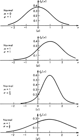
In this, its usual form, the mean and standard deviation (or variance) are used as parameters of the distribution, and we would write X is N(m,σ2).” The effect of changes in m and α is shown in Fig. 3.3.2. The normal curves plotted in dotted lines in Fig. 3.3.1 are those with mean and standard deviation equal to the corresponding moments of the true distributions.
Using normal tables The normal distribution is widely tabulated in the literature.† This job is simplified by tabulating only the standardized
Fig. 3.3.2 Normal density functions.
variable
This variable has mean 0 and standard deviation 1 (as the reader was asked to show in Prob. 2.47). The density of the standardized normal random variable is consequently N(0,1) or
which is shown in Fig. 3.3.2a. The desired density function, that of X = mX + σXU, is found using Eq. (2.3.15):
For example, the value of the density function in Fig. 3.3.2d at x = 1 is

Tables give only half the range of u, u ≥ 0, owing to the symmetry of the PDF.
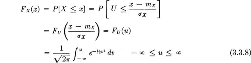
To determine the probability that a normal random variable lies in any interval, the integral of fX(x) over the interval is required; alternatively of course, the difference between the two values of the cumulative distribution function will yield this information. There is no simple expression for the CDF of the normal distribution, but it has been evaluated numerically and tabulated, again for the standardized random variable. In general
in which u = (x – mX)/σX. Note that u can be interpreted as the number of standard deviations by which x differs from the mean. Tables yield values of FU(u). Because of the symmetry of the PDF, tables give only half of the range of u, usually for u ≥ 0.
For example, the probability that a normal random variable X, with mean 4000 and standard deviation 400, will be less than 4800 is:
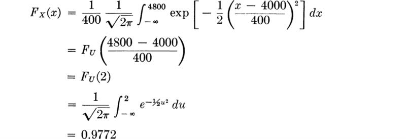
Concrete compressive strength is commonly assumed to be normally distributed, and a particular mix might have parameters near the values used here.
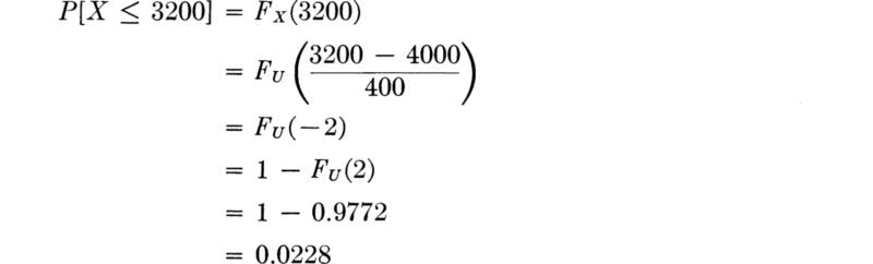
The symmetry of the distribution permits one to find values for negative arguments. A quick sketch should convince the reader that for the standardized normal variable,
Consequently, for the variable just cited:
In other tables 1 – FU(u) is tabulated for u ≥ 0, while still other tables give 1 – 2FU(– u), u ≥ 0.
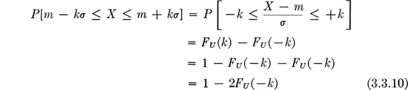
The last form is related to the common situation in the study of errors or tolerances where it is desired to know the probability that a normal random variable will fall within k standard deviations of its mean:
If one recalls the discussion in Sec. 2.4.1, he will recognize this value as the probability of a normal random variable remaining within the “k-sigma” bounds. In fact, the “rules of thumb” stated there are approximately those values one obtains for the probabilities of a normal variable. Therefore they are appropriate if the distribution is approximately bell-shaped.
Higher moments The symmetry of the normal distribution about its mean implies that all odd-order central moments (and the skewness coefficient) are zero. The even-order moments must be related to only the mean and standard deviation because these two moments serve as the parameters of the family of normal distributions. It can be shown by integration that the even-order moments are given by
Note that
Hence the coefficient of kurtosis [Eq. (2.4.19)] is
It is not uncommon to compare the coefficient of kurtosis of a random variable with this “standard” value of 3, that of the normal distribution. If a distribution has γ2> 3, it is said to be “flatter” than standard. In fact, one often sees defined the coefficient of excess, γ2 – 3. Positive coefficients of excess indicate distributions flatter than the normal, negative, more peaked than normal.
Distribution of the sum of normal variables Since by the central limit theorem the sum of many variables tends to be normally distributed, it should be expected that the sum of two independent random variables each normally distributed would also be normally distributed. That is, in fact, the case. The proof is a direct application of Eq. (2.3.45), but will not be demonstrated here. Accepting the statement, we conclude that the distribution of Z = X + Y when X is ![]() and Y is
and Y is ![]() is also normal if X and Y are independent. We can use the results of Sec. 2.4.3 to determine the parameters of Z:
is also normal if X and Y are independent. We can use the results of Sec. 2.4.3 to determine the parameters of Z:
Thus Z is ![]()
If we are interested in Z = X1 + X2+ · · · + Xn, where the Xi, are independent, normally distributed random variables, we can conclude, by considering pairs of the variables in sequence, that, in general, the sum of independent normally distributed random variables is normally distributed with a mean equal to the sum of their means and a variance equal to the sum of their variances. A generalization of this statement for nonindependent, jointly normally distributed random variables will be found in Sec. 3.6.2.
Illustration: Footing loads For example, suppose that a foundation engineer wanting to estimate the long-term settlement of a footing states that the total sustained load on the footing is the sum of the dead load of the structure and the load imposed by furniture and the occupancy loads. Since each is the sum of many relatively small weights, the engineer adopts the assumption that the dead load X and sustained occupancy load Y are normally distributed. Unable to see any important correlation between them, he also decides to treat X and Y as independent. Data from numerous buildings of a similar type suggest to him that
mX = 100 kips
σX = 10 kips
mY = 40 kips
σY = 10 kips
The distribution of the total sustained load, Z = X + Y, then is also normally distributed with mean
mz = 100 + 40 = 140 kips
and
![]()
A reasonable design load might be that load which will be exceeded only with probability 5 percent. This is the value z* such that
1 – Fz(z*)= 5 percent
or
Fz(z*)= 95 percent
In terms of U, the tabulated N(0,l) variable, we find u* = (z* – mz)/σz such that
FU(u*) = 95 percent
From tables,
u* = 1.65
implying that
z* = mz + 1.65σz
= 140 + (1.65) (14.1) = 163 kips
Applications It can be said without qualification that the normal distribution is the single most used model in applied probability theory. We have seen that a sound reason may exist for its adoption as a description of certain natural phenomena. Namely, it can be expected to represent those variables which arise as the sum of a number of random effects, no one of which dominates the total. As a consequence the normal model has been used fruitfully to describe the error in measurements, to represent deviations from specified values of manufactured products and constructed items that result from a number of pieces and/or operations each of which may add some deviation to the total, and to model the capacity of a system which fails only after saturation of a number of parallel, redundant (random capacity) components has taken place. Specific examples of the last case include the capacity of a road which is the sum of the capacities of its lanes, the strength of a collapse mechanism of a ductile, elastoplastic frame, which is a sum of constants times the yield moments of certain joints, and the deflection of an elastic material which is the sum of the deflections of a number of small elementary volumes. The normal model was adopted in Fig. 2.2.5 to represent the distribution of total annual runoff (given that it was not zero) based on the assumption that this runoff was the sum of a number of individual daily contributions.
The normal distribution is also often adopted as a convenient approximation to other distributions which are less widely tabulated. Those cases in which the normal distribution is a good numerical approximation can usually be anticipated by considering how this distribution arises and then invoking the central limit theorem. The gamma distribution with parameters λ and integer k, for example, was shown in Sec. 3.2.3 to be the distribution of the sum of k exponentially distributed random variables. For k large (integer or not) the normal distribution will closely approximate the gamma. Figure 3.2.4 shows that the approximation is not good for k ≤ 3 but that it rapidly improves as k increases.
Similarly, discrete random variables such as the binomial or Poisson variables can be considered to represent the sum of a number of “zero-one” random variables and can be expected, by the central limit theorem, to be approximated well by the continuous, normal random variable for proper values of their parameters. In particular, if the approximation is to be good for the binomial, n should be large and p not near zero or one, and for the Poisson, ν should be large. Figures 3.1.1 and 3.2.1 verify these conclusions. The ability to use the normal approximation may be particularly appreciated in such discrete cases where the evaluation of factorials of large numbers is involved. Many references treat these approximations in some detail (Hald [1952], Parzen [1960], Feller [1957], etc.)
Although certain corrections associated with representing discrete by continuous variables are available to increase the accuracy of the approximation, † it is usually sufficient simply to equate first and second moments of the two distributions (discrete or continuous) in order to achieve a satisfactory approximation. For example, the probability that X, a gamma-distributed random variable, G(12.5,3.16), is less than 3 is approximately equal to the probability that a normally distributed random variable, say X*, with the same mean, mX* = mX = 12.5/3.16 = 3.95, and same standard deviation, ![]() , is less than 3. That is, X* is N(3.95,(1.12)2). Thus
, is less than 3. That is, X* is N(3.95,(1.12)2). Thus
U is, as above, N(0,l). The exact value of FX(3) can be found using tables of the incomplete gamma function or of the χ2 distribution (Sec. 3.4). This value is 0.2000.
Whether the normal model is adopted following a physical argument or as an approximation to other distributions, it should be noted that its validity may break down outside the region about its mean. Tails of the distribution are much more sensitive to errors in the model formulation than the central region. Recall, for example, the original illustration, Fig. 3.3.1. To say that the sum of four uniformly distributed random errors is normally distributed is a valuable approximation in the range close to the mean, but it clearly falls down in the tails, where the normal distribution predicts a small, but nonzero probability of occurrence of errors larger than four units. The limits on the argument of a normal density function are theoretically plus and minus infinity, yet it may still be useful in practice to assume that some variable, such as load, weight, or time, which is physically limited to nonnegative values, is normally distributed. Caution must be urged in drawing conclusions from models based on such assumptions, if, as is often the case in civil engineering, it is just these extreme values (large or small) which are of most concern. In short, the engineer must never forget the range of validity of his model nor the accuracy to which he can meaningfully use it. This statement holds true for all probabilistic models, as well as for deterministic formulations of engineering problems, although it is too frequently ignored in both.
The ease with which one can work with the normal distribution, † its many tables, and its well-known properties causes its adoption as a model in many situations when little or no physical justification exists. Frequently it is used simply because an observed histogram is roughly bell-shaped and approximately symmetrical. In this case the reason for the choice is simply mathematical convenience, with a continuous, easily defined curve replacing empirical data. Even with little or no data, the normal distribution is often adopted as a “not-unreasonable” model. The American Concrete Institute specifications for concrete strength are based on the normal distribution because it seems to fit observed data. The U.S. Bureau of Public Roads, in initial development of statistical quality-control techniques for highway construction, has adopted the normal assumption for material and construction properties, often when no information is yet available. Such uses of the normal distribution serve a valid computational and operational purpose, but the engineer should be quick to question highly refined conclusions or high-order accuracy leading from such premises. ‡ In particular, results highly dependent upon the tail probabilities in or beyond the region where little data has been observed should be suspect unless there is a valid physical reason to expect the model to hold.
Multiplicative models While the normal distribution arose from the sum of many small effects, it is desirable also to consider the distribution of a phenomenon which arises as the result of a multiplicative mechanism acting on a number of factors. An example of such a mechanism occurs in breakage processes, such as in the crushing of aggregate or transport of sediments in streams. The final size of a particle results from a number of collisions of particles of many sizes traveling at different velocities. Each collision reduces the particle by a random proportion of its size at the time (Epstein [1947]). Therefore, the size Yn of a randomly chosen particle after the nth collision is the product of Yn–1 (its size prior to that collision) and Wn (the random reduction factor). Extending this argument back through previous collisions,
Also, a number of physical systems can be characterized by a mechanism which dictates that the increment Yn – Yn–1 in the response of the system when it is subjected to a random impulse of input Zn is proportional to the present value of the response Yn–1. Formally,
or

Letting Wi = 1 + Zi, this function is in the same multiplicative form as the breakage model above. The growth of certain economic systems may follow this model.
Finally, the fatigue mechanism in materials has been described as follows (Fruedenthal [1951]†). The internal damage Yn, after n cycles of loading, is
In this expression, Wn is the internal stress state resulting from the nth load application, subject to variation because of the internal differences in materials at the microscopic level. If, as a first approximation, g(Yn–1) is taken equal to cn–1 Yn–1,
Distribution In all these cases the variable of interest Y is expressed as the product of a large number of variables, each of which is, in itself, difficult to study and describe. In many cases something can be said, however, of the distribution of Y. Take natural logarithms ‡ of both sides of any of the equations above. The result is of the form
Since the Wi are random variables, the functions In Wi are also random variables (Sec. 2.3.1). Calling upon the central limit theorem, one may predict that the sum of a number of these variables will be approximately normally distributed. In this case, then, we expect In Y to be normally distributed. Let
Our problem is, knowing that X is normally distributed, to determine the distribution of Y or
A random variable Y whose logarithms are normally distributed is said to have the logarithmiconormal or lognormal distribution. Its form is easily determined.
In Sec. 2.3.1 we found that the density function in such a case of one-to-one, monotonic transformation is [Eq. (2.3.13)]

Here

and X is normally distributed:

Therefore, upon substituting,
The random variable Y is lognormally distributed, whereas its logarithm X is normally distributed. The range of Y is zero to infinity, whereas that for X is minus to plus infinity. If Y = 1, X = 0, and if Y > 1, X is positive. In the range of 0 ≤ Y ≤ 1, X is in the range minus infinity to zero, since the logarithm of a number between zero and unity is negative. Y cannot have negative values, since the logarithm of a negative number is not defined.
Common parameters In Eq. (3.3.24), for the PDF of Y, the parameters used, σX and mX, are the mean and standard deviation of X or In F, not of Y. A somewhat more natural pair of parameters involving the median of Y is available. The median ![]() of a random variable was defined in Sec. 2.3.1 as that value below which one-half of the probability mass lies. That is,
of a random variable was defined in Sec. 2.3.1 as that value below which one-half of the probability mass lies. That is,
![]()
When X equals In Y,
![]()
Thus,
In ![]()
For the normal and other symmetrical distributions, the median equals the mean: ![]() . Consequently,
. Consequently,
![]()
Thus
![]()
Substituting into Eq. (3.3.24) for In y – mX,
![]()
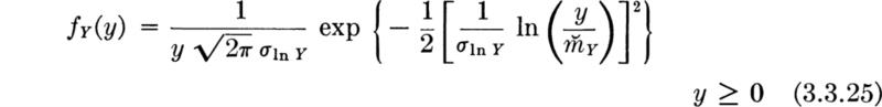
And, writing σX as σIn Y, we obtain the most common form of the lognormal PDF:
If y has this density function, we say Y is ![]() , where
, where ![]() and σIn Y are the two parameters of the distribution.
and σIn Y are the two parameters of the distribution.
Using normal tables In terms of the PDF of a standardized N(0,1) variable U,
That is,
where
The function fU(u) is widely tabulated.
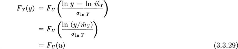
The CDF of Y is also most easily evaluated using a table of the normal distribution, since

Because X is N(mx,σX2) or ![]() ,
,
with u given above in Eq. (3.3.28).
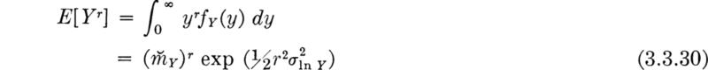
Moments Through experimental evidence one usually has available the moments of the random variable Y. To determine the parameters of the PDF and CDF, it then becomes necessary to compute ![]() and the standard deviation of X or In Y from these moments. To determine the equations to do this, we seek first the moments of Y in terms of its parameters. By integration, it is easily shown that the moments of Y are
and the standard deviation of X or In Y from these moments. To determine the equations to do this, we seek first the moments of Y in terms of its parameters. By integration, it is easily shown that the moments of Y are
In particular
and
Thus
It follows that the desired relationships for the parameters in terms of the moments are
It is also important to note that the mean of In Y or X is
The mean of In Y is not equal to In mY; that is, the mean of the log is not the log of the mean, illustrating again Eq. (2.4.29).
Illustration: Fatigue life From a number of tests on rotating beams of A285 steel, the number of cycles Y to fatigue failure were concluded to be lognormally distributed with an estimated mean of 430,000 cycles and a standard deviation of 215,000 cycles (when tested to ±36,400 psi). Let us plot fY(y) and FY(y). We are given from data
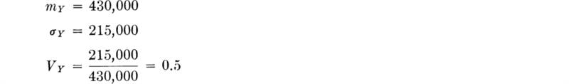
Using the previous results,

If VY is less than 0.2, one can assume that ![]() with less than 2 percent error in
with less than 2 percent error in ![]() . This follows from an expansion of ln
. This follows from an expansion of ln ![]() as
as
for VY < 0.2.
The other parameter of the lognormal distribution is

Again, if VY is less than 0.2, a good approximation is ![]() These two approximations can also be derived using the technique described in Sec. 2.4.4.
These two approximations can also be derived using the technique described in Sec. 2.4.4.
In this example, Eqs. (3.3.25) and (3.3.26) become
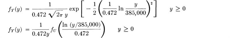
while the CDF is

Fig. 3.3.3 Lognormal distributions showing influence of σIn y.
To plot these functions, one might pick y at a number of selected locations and evaluate. It is somewhat easier, however, to select values of the standardized normal variable u, locate fU(u) and FU(u) in the tables, calculate the corresponding values of y, and finally compute fY(y). The functions fY(y) and FY(y) are shown graphed in Fig. 3.3.3. Also shown in Fig. 3.3.3 are plots of lognormal distributions with the same means but with coefficients of variation equal to 1.32 and 0.1. In these cases the parameters of the distributions are σInY, equal to 1.0 and 0.1, and ![]() equal to 260,000 and 429,800, respectively.
equal to 260,000 and 429,800, respectively.
Skewness and small V approximations Compared to a normal distribution, the most salient characteristic of the lognormal is its skewed shape. Through Eq. (3.3.30) the third central moment and thence the skewness coefficient of the lognormal distribution can be computed to be
Through Eqs. (3.3.38) and (3.3.35) it is clear that the coefficient ![]() and the skewness of the distribution depend only on the coefficient of variation of Y. The ratio of the mean to the median [Eq. (3.3.31)] also depends only on this factor. Furthermore, for small values of V (less than about 0.2), σIn Y and γ1 are very nearly linear in V [Eqs. (3.3.37) and (3.3.38)], and the mean of the logarithm of Y is approximately equal to the logarithm of the mean of Y. The distribution of Y is approximately normal for small V (Sec. 2.4.4).
and the skewness of the distribution depend only on the coefficient of variation of Y. The ratio of the mean to the median [Eq. (3.3.31)] also depends only on this factor. Furthermore, for small values of V (less than about 0.2), σIn Y and γ1 are very nearly linear in V [Eqs. (3.3.37) and (3.3.38)], and the mean of the logarithm of Y is approximately equal to the logarithm of the mean of Y. The distribution of Y is approximately normal for small V (Sec. 2.4.4).
Distribution of a product of lognormals The lognormal distribution does not have the additive regenerative property; that is, the distribution of a random variable which is the sum of two lognormal distributed random variables is no longer lognormal. But the distribution is rare in possessing a multiplicative type of regeneration ability. If
and the Yi are independent and all lognormally distributed with parameters ![]() and σInY, then Z is also lognormally distributed with
and σInY, then Z is also lognormally distributed with
and
By Eq. (3.3.36),
![]()
Hence
![]()
and
That Z is lognormally distributed follows [after logarithms of both sides of Eq. (3.3.39) have been taken] from the fact established in Sec. 3.3.1 that the distribution of the sum of independent normally distributed random variables is normally distributed. What is more, this argument also implies that under the same conditions on the Yi the random variable W:
is also lognormally distributed with easily determined constants.
Applications The lognormal probability law has a long history in civil engineering. It was adopted early in the statistical studies of hydro-logical data (Hazen [1914]) and of fatigue failures. It seems to have been adopted originally only because the observed data were found to be skewed, and better fit was obtained using this simple transformation of the familiar normal distribution. This skewed quality, † not uncommon in many kinds of data, plus the fact that the distribution avoids the nonzero probability (however small) of negative values associated with the normal model, have combined to make this distribution remain one commonly used in civil engineering practice. It is particularly frequently encountered in hydrology studies (for example, Chow [1954], Beard [1953], and Beard [1962]) to model daily stream flow, flood peak discharges, annual floods, and annual, monthly, and daily rainfall. Chow [1954] argues that the hydrological event is the result of the joint action of many hydrological and geographical factors which can be expressed in the mathematical form
![]()
where n is large. This form is typical of those which we have seen to lead to the lognormal distribution.
Lomnitz [1964] has used the multiplicative model to describe the distribution of earthquake magnitudes. He found the lognormal distribution to fit both the magnitudes and the interarrival times between earthquakes.
The distribution has also been found to describe the strength of elementary volumes of plastic materials (Johnso [1953]), the distribution of small particle sizes (Kottler [1950]), and the yield stress in steel reinforcing bars (Fruedenthal [1948]). A thorough treatment of the distribution is available in Aithchison and Brown [1957].
In civil engineering applications concern often lies with the largest or smallest of a number of random variables. Success or failure of a system may rest solely on its ability to function under the maximum demand or load to which it is subjected, not simply the typical values. Floods, winds, and floor loadings are all variables whose largest value in a sequence may be critical to a civil engineering system. The capacity, too, of a system may depend only on extremes, for example, on the strength of the weakest of many elementary components.
If the key variable Y is the maximum † of n random variables X1, X2, . . ., Xn, then the probability

If the Xi are independent,
In the special case where all the Xi are identically distributed with CDF FX(x):
If the Xi in the last case are continuous random variables ‡ with common density function fX(x),
Knowing from past experience the distribution of Xi the flood in any, say the ith., year, one might need the distribution of Y, the largest flood in 50 years, this being the design lifetime of a proposed water resource system. Equations (3.3.45) and (3.3.46) define the distribution of Y if the Xi can be assumed to be (1) mutually independent and (2) identically distributed. Related to these two assumptions are questions of long (multiyear) weather cycles, meteorological trends, changes (natural or man-made) in the drainage basin, etc. It may be possible to estimate the magnitude of these effects, if they exist, and, after alteration of the distributions of the Xi, make use of the more general form Eq. (3.3.44).
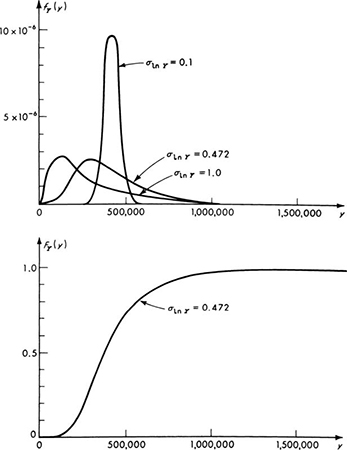
Fig. 3.3.4 Merging-traffic illustration. X values are times between vehicles.
Illustration: Merging lengths An engineer is studying how drivers merge into freely flowing traffic (Fig. 3.3.4). A certain class of drivers will merge only if the time Xi between passing cars is at least y sec. (The value of y will depend upon the class of drivers being studied.) If he assumes that the traffic is following a Poisson arrival process, then the Xi’s are independent, exponentially distributed random variables with parameter λ (Sec. 3.2). What is the probability that after n cars have passed, a driver will not have been able to merge?
Consider the maximum Y of the n times between cars, X1, X2, . . ., Xn. Then there will have been no merge if Y is less than y. For any particular value of y.
P[no merge] = ![]()
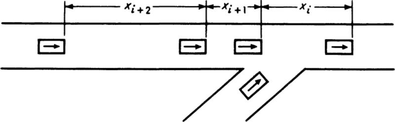
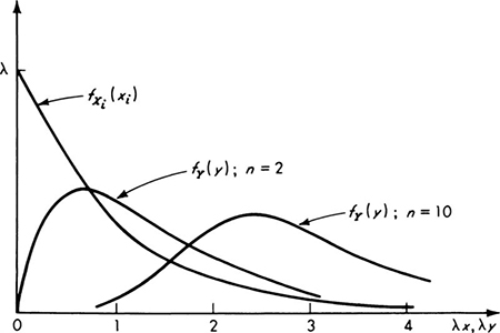
The density function of Y, the maximum of times, is simply
![]()
which is compared in Fig. 3.3.5 with the distribution of Xi for n = 2 and 10. Note that the maximum of say 10 values is likely to be (i.e., its mode is) in the right-hand tail of the distribution of Xi.
Fig. 3.3.5 comparison of PDF of interval times Xiwith that of maximum Y of n times.
Asymptotic distributions If the conditions of independence and common distribution hold among the Xi then in a number of cases of great practical importance the shape of the distribution of Y is relatively insensitive to the exact shape of the distribution of the Xi. In these cases, limiting forms (as n grows) of the distribution of Y can be found, which can be expected to describe the behavior of that random variable even when the exact shape of the distribution of the Xi is not known precisely. In this sense this situation is not unlike those already encountered in the previous two sections on the normal and lognormal distributions. When dealing with extreme values, however, no single limiting distribution exists. The limiting distribution depends, obviously, on whether largest or smallest values are of interest, and also on the general way in which the appropriate tail of the underlying distribution, that of the Xi behaves. Three specific cases, which have been studied in some detail (Gumbel [1958]) and applied widely, will be mentioned here.
Type I: Distribution of largest value The so-called Type I limiting distribution arises under the following circumstances. We wish to know the limiting distribution of the largest of n values of Xi as n gets large. Suppose that it is known only that the distribution of the xi is unlimited in the positive direction and that the upper tail falls off “in an exponential manner”; that is, suppose that, in the upper tail, at least, the common CDF of the Xi may be written in the form
with g(x) an increasing function of x. For example, if g(x)= λx, this is the familiar negative exponential distribution (Sec. 3.2.2). The normal and gamma distributions are also of this general type.
We have the following conclusion † for the distribution Y, the largest of many independent random variables with a common exponential type of upper-tail distribution:
and
The parameters α and u would be estimated from observed data in such cases. The result is asymptotic, being approximately true for any large value of n. For example, the engineer may argue that the annual maximum gust velocity has such an extreme-value distribution because it represents the largest of some unknown, but large number of gusts in a year (Court [1953]). A random variable with this, the Type I asymptotic extreme value distribution of largest values, will be said to be EXI,L (u,α) distributed. It is also called the Gumbel distribution, or simply the extreme-value distribution, when there is no opportunity for confusion with other extreme-value distributions.
Setting the derivative of fY(y) equal to zero will reveal that u is in fact the mode of the distribution. The parameter α is a measure of dispersion. Integration leads to the following expressions for the mean, variance, standard deviation, and third central moment of Y:
(γ is “Euler’s constant.”) Also
The skewness coefficient is
The distribution has a positive skewness coefficient which is independent of the parameters α and u.
The distribution is sketched in Fig. 3.3.6 in terms of a reduced
Fig. 3.3.6 Extreme-value distribution: type I, largest value.
variate W,†
This variable has u = 0 and α = 1.
Table A.5 gives the distribution tabulated in terms of this reduced variate.
The tables are used as those of the normal distribution are, since clearly
The use of the tables will be illustrated shortly.
Type I: Smallest value By a symmetrical argument one can find the distribution of the smallest of many independent variables with a common unlimited distribution with an exponential-like lower tail. Let Z be this minimum value; then the asymptotic (large n) distribution of Z is
with
The table for the distribution of largest values (Table A.5) may also be used for smallest values owing to the antisymmetry of the pair of distributions. In terms of the tabulated, reduced variate W [Eq. (3.3.54)]
and
![]()
used in tabulating and plotting the normal distribution.
Applications The Type I asymptotic extreme-value distribution has been used by a number of investigators to describe the strength of brittle materials (e.g., Johnson [1953]). The basic argument here is that a specimen of brittle material fails when the weakest of one of many microscopic, “elementary” volumes fails;† hence the distribution of smallest values is appropriate. The model is also commonly adopted to describe hydrological phenomena such as the maximum daily flow in a year or the annual peak hourly discharge during a flood (e.g., Chow [1952]), the reasoning being that the values are the maximum of many (365 in the first example) random variables. One might justly question whether the daily flows are independent or identically distributed, and certainly the daily flows cannot take on negative values. Nonetheless, the Type I distribution has proved useful to describe observed phenomena and seems to have some physical justification. Numerous other applications are referenced and discussed in Gumbel [1954a, 1958]. In Chap. 4 a special graph paper will be introduced that facilitates applications of this model.
As with the lognormal and normal models, having hypothesized the functional form or shape of the distribution, one would proceed to estimate parameters α and u (for example, from estimates of m and α). With these in hand one can make probability statements of the kind, “A flood of magnitude y will be exceeded with probability p in any given year,” or, “The strength which will, with 98 percent reliability, be exceeded z”
Illustration: Peak annual flow As an example, assume that an engineer has good estimates of the mean and variance of the peak annual flow in a small stream and that he suspects that the distribution is of the extreme-value type because the annual peak flow is the largest of many daily peak flows. He desires to plot the PDF of the assumed model in order to compare it with a histogram of the observed data. The mean and variance are given ‡:
mY = 100 cfs
σY2= 2500
σY = 50 cfs
Solving for the parameters α and u,
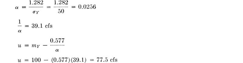
Now the engineer can compute, for example, the probability that the peak flow in a particular year will exceed, say, 200 cfs.

In order to plot the distribution of Y, one should read from the table (for various values of the reduced variate w) the values of fW(w) and FW(w). The corresponding values of y and fY(y) are easily found. The reduced variate is
W = (Y – u)α
Hence, a value w of W corresponds to a value of Y equal to

From Table A.5, we find:
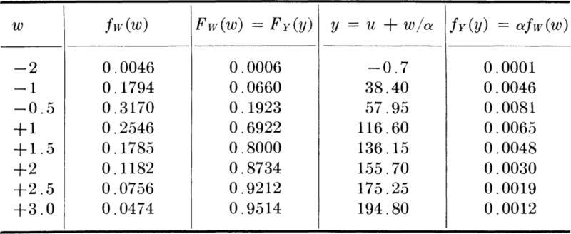
The PDF of Y is plotted in Fig. 3.3.7a.
Illustration: Minimum annual flows To illustrate the Type I distribution of smallest values, consider a distribution with the same mean and variance as used above for largest values. The distribution might now be the model of the minimum annual flow in a large stream. With
mz = 100 cfs
αz = 50 cfs
Fig. 3.3.7 Type I extreme-value illustrations, (a) Largest values; m = 100, α = 50; (b) smallest values, m = 100, σ = 50.
the parameters are
To plot the PDF of Z, values of the PDF of W at a number of values of its argument, w = 1.0, for example, are tabulated and the corresponding value of z found. For w = 1.0, fW(w) = 0.2546, and solving w = –α(z – u)= 1.0, we find the corresponding z equal to u – 1.0/α = 122.5 — 39.1 = 83.4. At z = 83.4, fz(83.4) = αfW(1.0) = (0.0256)(0.2546) = 0.0065. The entire PDF is plotted in Fig. 3.3.7. The indicated high probability of negative values suggests that the model is not a good choice if the physical variable Z is necessarily positive, as, say, a stream flow must be.
Type II distribution The Type II extreme-value distribution also arises as the limiting distribution of the largest value of many independent identically distributed random variables. In this case each of the underlying variables has a distribution limited on the left at zero, but unlimited to the right in the tail of interest. This tail falls off such that the CDF of the Xi is of the form
The asymptotic distribution of Y, the largest of many Xi, is of the form
We say Y is EXII,L(u,k).
Interestingly, the moments of order l of Y do not exist for l≥ k, but if l < k, integration yields
Consequently
Thus
This function of k only is plotted in Fig. 3.3.8, permitting one to find the parameter k if V is known from data.
The relationship between this distribution and the Type I distribution is identical to that between the lognormal and normal distributions. Using the technique of derived distributions, we can show that if Y has
Fig. 3.3.8 Extreme-value distributions. Coefficient of variation versus parameter k.
Type II distribution with parameters u and k, then Z = In Y has the Type I distribution [Eqs. (3.3.48) and (3.3.49)] with parameters u0 = In u and α = k. This fact can be utilized so that Table A.5 (and the special graph paper to be introduced in Chap. 4) can be used for Type II distributions as well as for Type I distributions. The relationship implies that
where Y is EXII,L(u,k) and Z is EXI,L(ln u,k). Thus in terms of the tabulated variable W, which is EXI,L(0,l),
A corresponding distribution of smallest values can also be found, but it lacks common practical interest.
This Type II distribution of largest values has been used (following Thorn [I960]) to represent annual maximum winds, owing to the physically meaningful limitation of the Xi to positive values and owing to the interpretation of the annual maximum wind velocity as being the largest of daily values, or perhaps the largest of many storms’ maxima, which are in turn the maxima of many gusts’ velocities. The distribution has also been employed to model meteorological and hydrological phenomena. (See references in Gumbel [1958].)
Illustration: Maximum annual wind velocity In Boston, Massachusetts, the measured data suggest that the mean and standard deviation of the maximum annual wind velocity are about
mY = 55 mph
σY = 12.8 mph
As mentioned, such velocities are suspected to follow the Type II extreme value distribution (although apparently no studies have been made to verify that the underlying distributions have the required shape in their upper tails). To find the parameters, we find first the coefficient of variation:
![]()
And from Fig 3.3.8
k = 6.5
while from Eq (3.3.69),
Standard mathematical tables yield Γ(0.846) = 1.12. Therefore
![]()
With the parameters known, probabilities can be calculated. For example, it has been recommended† that most structures be designed for the 50-year wind (see the illustration in Sec. 3.1). The velocity y, which will be exceeded with probability 1/50 = 0.02 in any year, is found by setting the complementary CDF of Y equal to 0.02:

Solving for y,
y = 91 mph
Alternatively, using Table A.5, we find that
FW(4.0) = 0.98
Using Eq. (3.3.74), this implies that
(In y – In 49.4)6.5 = 4.0
or
y = 91 mph
As indicated, this table can also be used to calculate values of fY(y)- For example,
With several values, the PDF of Y can be sketched as in Fig. 3.3.9.
Fig. 3.3.9 Type II extreme-value-distribution illustration.
Type III distribution The final asymptotic extreme-value distribution of interest is the Type III distribution, which arises from underlying distributions limited in the tail of interest. For example, if largest values are of interest and if the density function of the Xi falls off to some maximum value of w in a manner such that the following form of the CDF holds† near w
then the distribution of Y, the largest of many Xi, is of the form:
Since most useful applications of this model deal with smallest values, we shall restrict the remainder of the discussion to this case. We assume that the left-hand tail of the PDF of the Xi rises from zero for values of x ≥ ![]() such that the CDF has the following form near x =
such that the CDF has the following form near x = ![]() :
:
where ![]() is a lower limit of x. For example, the gamma distribution is known to be of this form (with
is a lower limit of x. For example, the gamma distribution is known to be of this form (with ![]() = 0). If the Xi are independent and identically distributed, the distribution of Z, the smallest or minimum of many values, is
= 0). If the Xi are independent and identically distributed, the distribution of Z, the smallest or minimum of many values, is
The moments are:
In many cases the primary purpose of experimental investigations may be to determine the lower limit e, a parameter of this distribution. For example, Weibull [1939] has studied material strength in tension and fatigue, ![]() representing the lower bounds on strength and on number of cycles before which no failures occur, respectively. Freuden-thal ([1951], [1956]) has given physical reasons why this model might hold in both cases. (Weibull’s justifications for its adoption were strictly empirical.) The distribution, with somewhat modified forms of the parameters, is often referred to as the Weibull distribution and is commonly employed in statistical reliability studies of the lifetimes of components and systems (see, for example, Lloyd and Lipow [1962].)
representing the lower bounds on strength and on number of cycles before which no failures occur, respectively. Freuden-thal ([1951], [1956]) has given physical reasons why this model might hold in both cases. (Weibull’s justifications for its adoption were strictly empirical.) The distribution, with somewhat modified forms of the parameters, is often referred to as the Weibull distribution and is commonly employed in statistical reliability studies of the lifetimes of components and systems (see, for example, Lloyd and Lipow [1962].)
In other cases, it may be reasonable to set ![]() = 0 simply from professional knowledge of the phenomenon of interest. Droughts have been studied in this manner (Gumbel [1954b]). If
= 0 simply from professional knowledge of the phenomenon of interest. Droughts have been studied in this manner (Gumbel [1954b]). If ![]() equals zero, the form of the distribution simplifies greatly, and we have
equals zero, the form of the distribution simplifies greatly, and we have
with
This last relationship is also graphed in Fig. 3.3.8.
In any case, a logarithmic transformation again permits the use of the tables of Type I. For, if Z is distributed following the Type III distribution of smallest values with parameters ![]() , u, and k [denoted EXIII, S(
, u, and k [denoted EXIII, S(![]() , u, k)], then X = In (Z –
, u, k)], then X = In (Z – ![]() ) has the Type I distribution of smallest values [Eqs (3.3.58) and (3.3.59)] with parameters u0 = In (u –
) has the Type I distribution of smallest values [Eqs (3.3.58) and (3.3.59)] with parameters u0 = In (u – ![]() ) and α = k; that is, X is EXI, S[ln (u –
) and α = k; that is, X is EXI, S[ln (u – ![]() ), k]. Thus
), k]. Thus
where W is the tabulated (Table A.5) EXI, L(0, l) variable. Consequently,
The illustration of the Type II distribution shows the steps in treating numerical examples.
General comments Some general comments concerning all three limiting extreme-value distributions are in order. † The results for the asymptotic distributions of extremes are not so powerful as those following from the central limit theorem for additive mechanisms. As we have seen, more assumptions must be made as to the general form of the underlying distributions. It may be difficult to determine which of the three forms [Eqs. (3.3.47) (3.3.65), or (3.3.76)] applies. Nor are these three forms exhaustive; distributions exist whose largest-value distribution does not converge to one of the three types given here. The effects of lack of independence and lack of identical distributions in the underlying variables are not so well understood as for the central limit theorem, but analogous conclusions (see Sec. 3.3.1) are known to hold (Juncosa [1948] and Watson [1954]). The convergence of the exact distribution [Eq. (3.3.44)] toward the asymptotic distribution may not be “fast” (Gumbel [1958]). Nonetheless, these distributions provide a valuable link between observed data of extreme events and mathematical models which aid the engineer in evaluating past results and predicting future outcomes.
In this section three general families of models have been studied. They share the common feature that they all arise when one is interested in a variable that is a consequence of many other factors whose individual behaviors are not well understood.
The normal or gaussian probability law

is the distribution of the sum of many random factors.
The lognormal distribution

describes the probabilistic behavior of the product of many random factors.
The extreme-value distributions are the distributions of the largest (or smallest) of many random variables. The particular form depends on the general analytical form of the corresponding tail of the distribution of these underlying variables.
In this section a number of other commonly encountered distributions are presented. Their utility stems in some cases from their ability to represent conveniently certain empirically observed characteristics of variables, such as both upper and lower limits. In other cases physical interpretations may be involved, some of which are considered here. Several of the distributions find their most frequent application in statistics, as will be discussed in Chap. 4.
If a random variable X is equally likely to take on any value in the interval 0 to 1, its density function is constant over that range
The shape of this density function is simply that of a rectangle, which gives it the name rectangular or uniform distribution. Its cumulative distribution function is triangular:
The mean and variance of the rectangular distribution are, by inspection,
Generalized slightly to an arbitrary range, say a to b, the density function becomes
when we denote it R(a, b). The mean and variance become
The distribution is commonly applied in situations where there is no reason to give other than equal likelihoods to the possible values of a random variable. † For example, the direction from which the earthquake shock waves may approach a proposed structure might be considered, in absence of information to the contrary, to be uniformly distributed on 0 to 360°. With respect to the signal’s cycle, the instant of arrival of an arbitrary vehicle at a traffic signal might be considered to be “at random” in the interval 0 to t0, where t0 is the duration of the signal’s cycle; and, if properly generated, a “random number”‡ can be considered to be uniformly distributed on the interval 0 to 0.999 ....
Distribution on 0 to 1 Although it can be shown to arise from the consideration of various underlying mechanisms, § the beta distribution, BT(r, t) is presented here simply as a very flexible distribution for use in describing empirical data. Like the simple rectangular distribution, it is limited in its basic form to the range 0 ≤ x ≤ 1. For r and t – r positive, the beta distribution is
where the normalizing constant is
if r and t – r are integer-valued, or
if r and t – r are not restricted to being integer-valued.¶
The mean of the beta distribution is
while
The skewness coefficient is
Shapes The great value of the beta distribution lies in the wide variety of shapes it can be made to assume simply by varying the parameters. It contains as special cases the rectangular distribution (r = 1, t = 2) and triangular densities (t = 3 and r = 1 or 2). It is symmetrical about x = 0.5 if![]() . The beta distribution is skewed right if
. The beta distribution is skewed right if ![]() and left if
and left if ![]() It is U-shaped if r < 1 and t ≤ 2r; it is J-shaped jf r < 1 and t > r + l or if r>l and t < r + 1. It is unimodal and bell-shaped (generally skewed) if r > 1 and t > r + 1, with the mode at x = (r– 1)/t – 2. Concentration about a fixed mode position increases as the values of the parameters are increased. Interchange of parameters, r' = t – r and t' = t, yields mirror images. Many of these relationships are displayed in Fig. 3.4.1.
It is U-shaped if r < 1 and t ≤ 2r; it is J-shaped jf r < 1 and t > r + l or if r>l and t < r + 1. It is unimodal and bell-shaped (generally skewed) if r > 1 and t > r + 1, with the mode at x = (r– 1)/t – 2. Concentration about a fixed mode position increases as the values of the parameters are increased. Interchange of parameters, r' = t – r and t' = t, yields mirror images. Many of these relationships are displayed in Fig. 3.4.1.
Tables For integer-valued t and r one can use tables of the binomial distribution to evaluate fX (x) or FX (x). As a function of y, n, and p the distribution of a binomial random variable Y is

which, when compared to the beta distribution
suggests why
if pY (y) is evaluated for n = t – 2 and y = r – 1 for various values of p = x. For example, if it is desired to find fX (x) when X is BT(1, 4), then it equals 3pY (0) for F-distributed B(2, x). In particular,

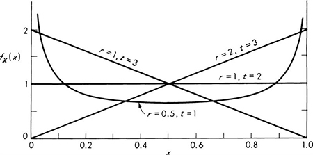
Fig. 3.4.1 Beta-distribution shapes.
in which 0.36 = P[Y = 0] when Y is B(2, 0.4). The equality is verified by substituting values of r, t, x, and m, p, y in the respective PDF and PMF of X and Y.
Similarly, one can verify that
where X is BT(r, t) and Y is B(t – 2, x).
For noninteger r and t, interpolation is possible, or more general tables must be used (e.g., Benjamin and Nelson [1965] or Thompson [1941]). A small table for some noninteger values of r and t is reprinted as Table A.4.
Beta distribution on a to b Although variables of interest may be distributed on the interval 0 to 1, it is common to want to use other limits on the range of the variable, say a to b. In this case, the beta distribution BT(a, b, r, t) generalizes to
when
It is apparent that a simple linear relationship exists between Y, a BT(a, b, r, t) variable, and X, a BT(0, l, r, t) [or BT(r, t)] variable. In particular,
Consequently to find CDF and PDF of Y from the tabulated values of X, we use the familiar results for linear relationships (Sec. 2.3.1):
Illustration: Wind direction For planning runway directions or for studying dispersions of air pollutants from power plants, both the “prevailing” wind direction and the random variations in the direction are critical. The wind direction Y at the Boston airport measured in degrees from north has mean and standard deviation of about

These are the averages of many observations at many different hours, days, and seasons. The direction is of course limited between 0 and 360°. Thus, assuming that a beta distribution is appropriate,
![]()
Thus Y is BT(0, 360, 1.25, 2.2), and its density function is

where X is BT(1.25, 2.2). The tabulated density BT(1.2, 2) is sketched in Fig. 3.4.2. A histogram of observed wind directions is sketched to the same scale. Although the comparison with data is not bad, the shape of this beta distribution is not satisfactory physically. The sharp discontinuity between the values of fY at 0 and 360°, which are both the same direction, north, is an unrealistic but perhaps not important feature of the model.
Fig. 3.4.2 Wind-direction illustration.
A number of important distributions arise as a consequence of operations on normal distributions. They are most commonly encountered in statistical applications (Chap. 4), but their derivations are simply problems of probability theory of the type studied in Sec. 2.3.
The chi-square distribution The most important of these normal-related distributions describes the distribution of Yν the sum of the squares of ν independent normal random variables. Consider the case first of only one normal variable
![]()
where X1 is 2V(0, 1). Using the techniques of Sec. 2.3,
Therefore,
The distribution of Yν could be found by successive convolutions (Sec. 2.3.2) of the distribution of Y1 but it is simpler to recognize, comparing Eqs. (3.2.18) and (3.4.24), that fy1(y) is gamma-distributed with ![]() and
and ![]() (
(![]() ). But recall (Sec. 3.2.3) that the sum of ν independent G(k, λ) gamma variables (with common X) is gamma-distributed with kv = Σki = vk; that is, the sum is G(νk, X). It is therefore clear that Yv the sum of v squared independent normal random variables, is
). But recall (Sec. 3.2.3) that the sum of ν independent G(k, λ) gamma variables (with common X) is gamma-distributed with kv = Σki = vk; that is, the sum is G(νk, X). It is therefore clear that Yv the sum of v squared independent normal random variables, is ![]() , with PDF [Eq. (3.2.18)]
, with PDF [Eq. (3.2.18)]
This distribution is called the chi-square or χ2 distribution, † with parameter ν or with ν “degrees of freedom”, and is denoted here as CH(ν). From its derivation it is clear that the distribution is regenerative; the distribution of ![]() is CH(ν 1 + ν2). It is plotted in Fig. 3.4.3. These plots and the central limit theorem (Sec. 3.3.1) suggest that the χ 2 distribution can be closely approximated by a N(ν, 2u) distribution for larger values of ν.
is CH(ν 1 + ν2). It is plotted in Fig. 3.4.3. These plots and the central limit theorem (Sec. 3.3.1) suggest that the χ 2 distribution can be closely approximated by a N(ν, 2u) distribution for larger values of ν.
Fig. 3.4.3 x2 distributions. (Adapted from R. S. Burington and D. C. May, “Handbook of Probability and Statistics, ” Handbook Publishers, Inc., Sandusky, Ohio, 1953.)
χ 2, gamma, and Poisson tables The cumulative χ 2 distribution is found tabulated in Appendix A.2. Values of the cumulative distribution of a χ 2 random variable can be read directly. For example, from the table, the probability that a χ 2 random variable with ν = 6 degrees of freedom is less than 1.1 is
![]()
The table also provides the means to evaluate the CDF of a gamma-distributed random variable. As shown above, if Z is G(k, λ), then Y = 2λZ is CH(2k) (if 2k is integer). Hence the CDF of Z is
where FY is tabulated. For example, if Z is (G (1.5, 2), i.e., gamma with k = 1.5 and λ = 2, then

where Y is CH(3), i.e., χ 2-distribution with ν = 2k degrees of freedom. Looking in the tables of the χ 2 distribution with ν = 3, FY(4.0) is found to be
![]()
The cumulative distribution of a discrete Poisson random variable X with mean (parameter) m can also be evaluated using this table.
Thinking in terms of a Poisson process with average rate λ, X is the number of arrivals in time t = m/λ (since m = λt, Sec. 3.2.1). But the probability that x or fewer arrivals occur in time t is equal to the probability that Z, the waiting time to the (x + l)th event, is greater than t:

But Z is gamma-distributed with parameters k = x + 1 and λ; therefore, from above Fz(t) = FY(2λt) in which Y is a χ 2 random variable with ν = 2k = 2(x + 1) degrees of freedom. Finally, substituting t = m/ λ,
![]()
where FY is tabulated. For example, if X is Poisson-distributed with mean m = 1.3, then the probability that X ≤ 3 is
![]()
where Y is CH(8); that is, Y is χ 2-distributed with ν = 2(3 + 1) = 8.
From Table A.2 with v = 8,
![]()
The chi distribution If the χ2 distribution represents the sum of the squares of two, say, independent N(0, l) random variables, and these latter two variables are, for example, the errors in the N-S and in the E-W directions in a surveying measurement, then the distribution of the square root of this sum of squares is of interest as the distribution of the actual amplitude of the error, regardless of direction. If Y is CH(ν), and ![]() ,
,
which indicates how one may use χ 2 tables to evaluate the CDF of X. Also,
This distribution is known as the chi or χ distribution. Its mean is
Since
![]()
and since
![]()
it follows from Eq. (3.4.26) for the mean of Y that
We shall denote the χ distribution by CHI(ν).
The t and F distributions Two other distributions that are related to normal random variables should be mentioned here. These are the Student’s t distribution and the F distribution.
The former, denoted here T(ν), is the distribution of the ratio of X, a N(0, l) random variable, to ![]() , where Y is an independent χ-distributed random variable, CHI(ν). That is,
, where Y is an independent χ-distributed random variable, CHI(ν). That is, ![]() is a normal random variable divided by the square root of the sum of v squared, independent, standardized normal random variables (the sum being normalized first by its mean.) The density of Z can be derived to be (for ν > 2)
is a normal random variable divided by the square root of the sum of v squared, independent, standardized normal random variables (the sum being normalized first by its mean.) The density of Z can be derived to be (for ν > 2)
The t distribution is symmetrical about zero, having almost normal-looking shapes for large values of v (Fig. 3.4.4). Its mean is zero and its variance is
The cumulative t distribution is tabulated (Table A.3), but it is clear from Fig. 3.4.4 that for reasonably large values of ν the distribution can be approximated by a N(0, ν/(ν – 2)) distribution. The t distribution is found almost solely in statistical applications (Sec. 4.1), but it has been employed to describe empirically the strength of structural assemblies by Freudenthal, Garrelts, and Shinozuka [1966].
Fig. 3.4.4 The t distribution. (From A. Hald, “Statistical Theory with Engineering Applications, ” John Wiley & Sons, New York, 1952.)
The final normal related distribution of interest is the F distribution. If X and Y are independent χ2 random variables with degrees of ν1 and ν2, respectively, then the F distribution is the distribution of the ratio of
In words, the ratio of the sum of the squares of ν1 N(0, l) random variables to the sum of the squares of ν2 N(0, l) random variables (the sums being divided by their means) can be determined to be
We shall denote the F distribution by F(ν1ν2), being careful to avoid confusion with the joint CDF of a pair of random variables. Its mean is
and its variance is
The F distribution is widely tabulated; Table A.6 gives only the value of z which is exceeded with probability 5 percent. The shape of the density function is similar to that of the χ2 distribution which it approaches as ν2 grows. This distribution also finds its primary application in statistical procedures (Chap. 4).
Illustration: Random vibrations If a simple linear 1-degree-of-freedom oscillator like that pictured in Fig. 3.4.5c is acted on by a forcing function F(t), its dynamic response X(t) (from rest at time zero) is well known from mechanics to be
where ω is the natural (circular) frequency of the oscillator and F(t) is measured in units of force per unit mass. A similar form of the convolution (or Duhamel) integral holds if F(t) is a ground acceleration. A number of engineers (see, for example, Rodriguez [1956]) have proposed that the dynamic response of structures to earthquakes might be represented by treating the ground acceleration as a sequence of evenly spaced impulses Fi, i = 1, 2, . . ., of random magnitude (assumed for simplicity here to be independent and identically distributed) (Fig. 3.4.5a). Similar approaches have been taken to represent the response of towers to wind (Chiu [1964]). In such cases, the integral
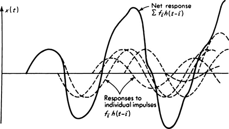
Fig. 3.4.5 Random-vibration illustration, (a) Typical sample of forcing function; (b) dynamic response to typical sample of forcing function; (c) simple oscillator representation of a structure.
reduces to a sum (Fig. 3.4.5b) which we can write as
where h(t – i) is the response of the structure t – i time units (say seconds) after an impulse of unit magnitude strikes the structure.
For our purposes here it is sufficient to recognize simply that the response Xt is the sum of a number of random variables, Fih(t – i), and under many circumstances might, by the central limit theorem, be assumed to be normally distributed, N(0, σt2). The mean response is assumed to be zero, a reasonable assumption if the earthquake accelerations are symmetrically distributed about zero or if we are dealing with dynamic response to fluctuations in the wind (about a mean velocity to which response is static). The variance is proportional to the assumed common variance of the Fi [Eq. (2.4.81)]. In a similar fashion the velocity of the system ![]() t = dX/dt can be represented as
t = dX/dt can be represented as
where g(t – i) is the derivative of h(t – i). ![]() t, too, might often be expected to be normally distributed. It can be considered to have zero mean, and its variance is approximately ω2σt2 A somewhat surprising result of this theory of random vibrations is that under many practical circumstances, after the initial starting conditions have been damped out, Xt and
t, too, might often be expected to be normally distributed. It can be considered to have zero mean, and its variance is approximately ω2σt2 A somewhat surprising result of this theory of random vibrations is that under many practical circumstances, after the initial starting conditions have been damped out, Xt and ![]() t are independent random variables. †
t are independent random variables. †
Energy If we seek the distribution of the energy Et in the system at time t, it is simply the sum of the kinetic energy of the mass and the potential energy stored in the spring:
in which m is the mass and k the spring constant of the oscillator. Then

or, since ![]()

Multiplying and dividing by σt2,

or
Since Xt is N(0, σt2) and ![]() t is iV(0, ω2σt2), the variables on the right-hand side are the squares of independent N(0, l) random variables; hence 2Et/k σt2 is χ2-dis-tributed with ν = 2. Given information regarding the intensity or gustiness of the forcing function, which can be interpreted in terms of the variance of the Fi and subsequently the σt2, one can compute the probability that the energy in the system at time t will exceed any critical value, since
t is iV(0, ω2σt2), the variables on the right-hand side are the squares of independent N(0, l) random variables; hence 2Et/k σt2 is χ2-dis-tributed with ν = 2. Given information regarding the intensity or gustiness of the forcing function, which can be interpreted in terms of the variance of the Fi and subsequently the σt2, one can compute the probability that the energy in the system at time t will exceed any critical value, since
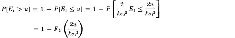
where Y is CH(2). Recall that a CH(2) distribution is equivalent to a gamma distribution, ![]() , which in turn is simply an exponential distribution with parameter
, which in turn is simply an exponential distribution with parameter![]() . Thus, from Eq. (3.2.8),
. Thus, from Eq. (3.2.8),

In short, the energy in the system at any time t is exponentially distributed, EX(1/kσt2).
Amplitude A second response characteristic of interest is the amplitude of vibration
It is shown in elementary dynamics that if the system were in free vibration, At would be the maximum value of Xt; consequently it is significant as an indicator of the maximum displacement (and hence strains and stresses) which the system will undergo. By an argument similar to that above
is the square root of the sum of the squares of two independent N(0, l) random variables and hence is χ-distributed with 2 degrees of freedom. Letting Z = (l/ σt)At, we know that Z is CHI(2):
![]()
At is linearly related to Z:
This special case of the χ distribution is usually referred to as the Rayleigh distribution. Its shape is plotted in Fig. 3.4.6Fig. 3.4.6. As mentioned earlier, the χ2 tables can be used to evaluate χ CDF’s.
where Z is CHI(2) and Y is CH(2) or ![]() . Thus
. Thus
Fig. 3.4.6 Rayleigh or χ (with ν = 2) distribution.
which could have been determined by integrating ![]() Evaluation of Eq. (3.4.49) for a critical value of a (say the value of displacement at which cracking of plaster or damage to windows will occur), will determine approximately the likelihood of this event at or near time t. †
Evaluation of Eq. (3.4.49) for a critical value of a (say the value of displacement at which cracking of plaster or damage to windows will occur), will determine approximately the likelihood of this event at or near time t. †
Several common models are catalogued in this section. They were two limited distributions:
1. The uniform distribution
![]()
and
2. The beta distribution,

and four distributions of functions of independent normal random variables:
3. The chi-square (χ 2) distribution, which is the distribution of sum of ν squared normal variables.
4. The chi (χ) distribution, which is the square root of the sum of the squares of ν normal variables.
5. The t distribution, the ratio of a N(0, l) variable to the square root of the sum of ν squared N(0, l) variables divided by ν.
6. The F distribution, the ratio of the sum of ν1 squared N(0, 1) variables (divided by ν1) to the sum of ν2 squared N(0, l) variables (divided by ν2).
A number of modifications to the more common distributions presented in the earlier sections of this chapter are frequently adopted in order to relate the mathematical model more closely to the physical problem or simply to provide a better empirical fit to observed data.
Shifts The simplest modification to a distribution is simply a shift of the origin. For example, the exponential interarrival time between vehicles has been found to be a satisfactory model even in fairly dense traffic if it is shifted an amount t0 to account for the impossibility of vehicles arriving within time intervals on the order of the length of a vehicle divided by its velocity. Thus the engineer would assume T – t0 to be exponentially distributed, implying
which is plotted‡ in Fig. 3.5.1.
A similar shift has been used by Chow and Ramaseshan [1965] with the lognormal distribution to describe hydrologic data. The shifted gamma has been used by Vorlicek and Suchy [1958] to describe the strength of concrete and steel and by Markovic [1965] to describe maximum annual flows. In most such cases the shift was introduced not because the author had reason to believe that there was a natural lower bound, but rather simply to gain an additional parameter (three rather than two in the case of the lognormal and gamma distributions) to insure a better fit to the data. Markovic [1965], in fact, compared (using a method to be discussed in Sec. 4.5) the closeness of the fit produced by the two- and three-parameter gamma and lognormal distributions to many different rivers’ records of annual maximum flows. Notice that the parameters w and e in the Type III asymptotic extreme-value distributions (Sec. 3.3.3) can, in fact, be considered as simply shift parameters added to basically two-parameter distributions.
Fig. 3.5.1 Shifted exponential distribution.
The mean of the shifted distribution is simply the original mean plus the shift. All central moments such as the variance are unchanged.
The simple shift is, of course, no more than a special case of the linear transformation
which was seen in Sec. 2.3.1 to leave the shape of the distribution unchanged but to cause a shift to the right (if x0 > 0) by x0 and a scale expansion (if b > 1) by a factor b. The density of Y if X is a continuous random variable was found to be simply
Such linear transformations have been used to reduce distributions (e.g., the normal, Sec. 3.3.1, or the gamma, Sec. 3.2.2 and 3.4.3) to standardized forms more easily tabulated.
Transformations More general transformations are commonly used if professional knowledge so indicates or if better fits to observed data result. Examples of the former case included the lognormal distribution (Sec. 3.3.2), where, if a multiplicative mechanism is indicated, it may be reasonable to assume that the logarithm of the variable of interest is normally distributed. Examples of the latter case, transformations for convenience, include the assumption by Stidd [1953] and Beals [1954] that Xa is normally distributed where X is the total precipitation during a fixed period.† In general, of course, the greater the number of independent parameters available for estimating from data (Chap. 4) the better the fit that can be expected.
Many of the distributions given special names in the previous sections of this chapter can be recognized as no more than cases where some function of the variable has one of the other distributions. In many cases they were derived this way. For example, if the distribution of X is assumed to be χ2-distributed, then the distribution of ![]() is χ-distributed. Notice, too, that if
is χ-distributed. Notice, too, that if

is assumed to be exponential with parameter λ = 1, one is led to the conclusion that X has the Type III asymptotic extreme-value distribution, since
![]()
Similarly, if ![]() is assumed to be exponentially distributed, X has the Type I extreme-value distribution. Knowledge of such relationships can often simplify problem solutions.
is assumed to be exponentially distributed, X has the Type I extreme-value distribution. Knowledge of such relationships can often simplify problem solutions.
Truncated distributions In certain situations tails of distributions may be “lost” owing, say, to an inspection procedure which leads to the elimination of all those members of the population of manufactured items or mixed materials, for example, with values less than a particular value x0. Such a distribution is said to be truncated below x0. The resulting distribution might then have a shape like that in Fig. 3.5.2 if the distribution of the original population was normal, for example.
If the original population had PDF fX (x) and CDF FX (x) and if the variable of interest Y has been truncated below x0, its PDF is zero
Fig. 3.5.2 The truncated normal distribution.
up to x0 and fX (x) is renormalized† for x ≥ x0:
where k = 1/[1 – FX (x0)]. Similar results hold if the upper tail is truncated or if both tails are truncated.
Truncated distributions have been employed by Fiering [1962] (the normal) to describe hydrologic data, by Das [1955] (the gamma) to describe daily precipitation, and by Freudenthal, Garrelts, and Shinozuka [1966] (the t distribution) to describe the ultimate capacity of structural members.
Censored distributions Censored distributions differ slightly in application in that the total population is present but the exact frequencies are known only up to (or beyond) a certain value x0. For example, in fatigue testing it is not uncommon at low stress levels to stop the test of long-lived members short of failure at an arbitrary, high, number, say 106 cycles, simply to free the apparatus for further testing. The observed failures and the unfailed specimens represent samples from a population characterized by the parent or underlying population up to the cutoff value x0, but of unspecified magnitude (other than greater than x0) beyond this cutoff point. When, as in many engineering applications, the nature of the underlying distribution is being determined from observed data, it is wasteful and improper to neglect the information that a certain proportion of the observations exceeded x0 in value. In many cases the distribution is assumed to have the probability or proportion above x0 lumped at x0. If the underlying distribution is continuous, the censored distribution is mixed with a spike at x0. See, for example, the pump-capacity illustration in Sec. 2.4.2. Such questions are treated in Hald [1952].
Compound distributions arise when a parameter of the distribution of a random variable is itself treated as a random variable.
Illustration: Vehicle delays during construction operations For example, assuming vehicle arrivals on a rural road are Poisson events (Sec. 3.2.1), closing the road for a construction operation for t min will lead to the delay of X vehicles. X has the Poisson distribution with parameter λt, where λ is the average number of cars arriving per minute:
Suppose now that, since it may be caused by one of a number of different operations, the duration of the closed period is a random variable with a probability mass function pT (t) that is related directly to the relative likelihood that a particular operation taking a particular time causes the closure. Then, considering all possible values of t, each with its relative likelihood, the number of cars stopped by an arbitrary unspecified type of closure has distribution
If each of the operations takes a random amount of time, it is reasonable to treat T as a continuous random variable when the previous equation becomes
For example, if T is exponentially distributed with parameter α,
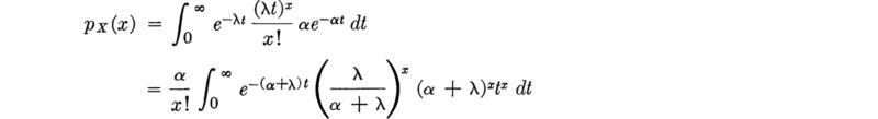
Letting u = (α + λ)t,

The integral is by definition Г(x + 1), which for integer x is x!. Thus
Fig. 3.5.3 Geometric distribution arising from vehicle-delay illustration.
which coincidently is simply the geometric distribution† (Sec. 3.1.2) with parameter α./(α + λ). For example, if the mean arrival rate is λ = 3 cars per minute and the average delay is 1/ α = 1 min, ![]() The mean number of cars stopped is 4 – 1 = 3, which is intuitively satisfactory; the distribution of X is plotted in Fig. 3.5.3. Notice that the geometric distribution does not arise here from the argument about the number of Bernoulli trials preceding the first success, which was used in Sec. 3.1.3. The illustration was included here to emphasize that totally different underlying mechanisms may lead to the same distribution. Therefore one cannot infer conclusively that a particular mechanism is acting if observed data appear to follow a particular distribution.
The mean number of cars stopped is 4 – 1 = 3, which is intuitively satisfactory; the distribution of X is plotted in Fig. 3.5.3. Notice that the geometric distribution does not arise here from the argument about the number of Bernoulli trials preceding the first success, which was used in Sec. 3.1.3. The illustration was included here to emphasize that totally different underlying mechanisms may lead to the same distribution. Therefore one cannot infer conclusively that a particular mechanism is acting if observed data appear to follow a particular distribution.
General form In general, if a random variable X has CDF FX (x) which depends upon a parameter θ [and which therefore might be written FX (x;θ)], then we can find the CDF of another random variable Y when θ is a random variable‡ as follows:
or
depending on whether θ is discrete or continuous. If Y is discrete, which it will be if X is, its PMF can be found by replacing FX (x) by pX (x). Similarly, as was done in the previous illustration, the PDF of Y can be found by putting the PDF of X in place of its CDF in Eqs. (3:5.9) and (3.5.10). The distribution of Y is just the weighted average of the distributions of X for each value θ.
Illustration: Uncertain supplier of material The simple case when the parameter has a discrete distribution, Eq. (3.5.9), is simply a formal way of treating situations where the engineer may be faced with uncertainty as to which of several distributions is applicable. Then the values of pθ(θ) can be interpreted as the engineer’s weights or degree-of-belief assignments (see Sec. 2.1.2) as to the true distribution. For illustration, a job’s material may be furnished by one of two manufacturers, each producing material with his own characteristic distribution, the two being different in means, variances, and, possibly, shapes. Knowledge of these distributions and the relative likelihoods of receiving the material from each manufacturer will yield by Eq. (3.5.9) a material property distribution which accounts for uncertainty in the supplier. For example, if two contractors just meet ACI specifications† for 4000-psi concrete, but one produces material with a coefficient of variation V1 = 10 percent, while the other’s concrete has V2 = 15 percent, then the probability that the supplied strength will be less than 3500 psi is (assuming, as ACI does, normal distributions)
![]()
if 0.2 and 0.8 are the respective likelihoods that contractors 1 and 2 will get
Fig. 3.5.4 Bimodal PDF from illustration involving uncertain supplier of materials.
the job. In this case, letting U be N(0, l),
It should be clear that Y is not normally distributed, but, in fact, is a bimodal distribution having peaks near 4600 and 5000 psi:
This density function is shown in Fig. 3.5.4.
Moments Although the distributions resulting from compounding or “mixing” may be difficult to determine analytically, owing to the integration or summation involved, the moments are more easily found. It is readily shown through substituting into their definitions, Eq. (2.4.16), that the moments about the origin are simply
or
where ![]() is the nth moment of X given that the parameter of the distribution of X is θ. In particular, †
is the nth moment of X given that the parameter of the distribution of X is θ. In particular, †
The mean of Y is just the weighted average of the means of X for the various values of θ. In terms of mY and![]() , the variance we know to be
, the variance we know to be

Substitution and manipulation let the variance of Y be written
which makes it clear the variance of Y is not the weighted average of the variances of X for the various values of θ. Engineers will see an analogy with the parallel-axis theorem for obtaining the moment of inertia of an area made up of several small areas, †
Similar relationships hold for the first and second moments of Y when the distribution of 9 is continuous.
Illustration: Total rainfall As a final illustration of compound distributions, recall the illustration in Sec. 2.3.3. There we sought the distribution of the total annual rainfall T, when the number of rainy weeks N is Poisson-distributed with mean v = 20 and the rain in a rainy week is exponentially distributed with parameter λ = 2 in.-1 (or mean ![]() in.). In that section a Monte Carlo technique was used to solve the problem. Using the notions of compound distributions, we can find the distribution of T directly.
in.). In that section a Monte Carlo technique was used to solve the problem. Using the notions of compound distributions, we can find the distribution of T directly.
If the number of rainy weeks were known, the distribution of T would be gamma, G(n, λ), since the sum of n (assumed independent and identically distributed) exponential random variables is gamma (Sec. 3.2.3).
if n > 0. (If n = 0, T = 0.) The parameter n of this gamma distribution is Poisson-distributed‡; hence, for t > 0,
The distribution of T is a mixed distribution. Equation (3.5.18) gives the continuous part. At t = 0, we must include a spike, a finite probability of exactly zero rainfall, if there are no rainy weeks. The magnitude of this spike is simply ![]() .
.
Simplifying Eq. (3.5.18) and letting u = n – 1,
This density could be evaluated numerically§ for a set of values of t. The distribution of T is sketched in Fig. 3.5.5 for v = 20 and λ = 2. Note that the continuous part is approximately normal, as should be expected. This is clearly one reasonable form for a model of the problem and data discussed in Sec. 2.2.1. The mean and variance of T are, by Eqs. (3.5.15) and (3.5.16)

Fig. 3.5.5 Mixed PDF of total annual rainfall.
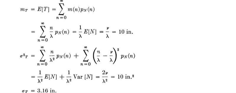
Recall that the mean and variance of T were also calculated in Sec. 2.4.3 by an alternate approach.
Common distributions are often modified in various ways to extend their usefulness in applications. These modifications include:
1. Transformations:
A function Y = g(X) of the variable of interest is assumed to have a particular common distribution. A frequent case is Y = X – a, which leads to a shift of the common distribution.
2. Tail modifications:
The probability mass in a tail (or tails) of the common distribution may either be removed (truncated) or lumped at the cutoff point (censored).
A new distribution may be formed by treating θ, the parameter(s) of a common distribution, as a random variable. In this case the distribution becomes a weighted distribution
![]()
Clearly, many different multivariate models can be formed easily from the common univariate models discussed in the previous sections of this chapter. For example, in Sec. 2.2.2, a Poisson marginal and binomial conditional distribution led to a joint distribution of the number of arriving vehicles and the number of counted vehicles when the counter was defective. Also, reexamination of the models formed from compound distributions will make it clear that the integrand in such an equation as [see Eq. (3.5.10)]
is simply the joint density function of Y and θ since it can be interpreted as the product of the conditional distribution of Y given θ and the marginal distribution of 6 (Eq. 2.2.45a). In the annual-rainfall illustration of Sec. 3.5.3, for example, extracting the function from under the summation sign in Eq. (3.5.18) yields the joint distribution of the total rainfall T and the total number of rainy weeks N:
which is continuous in t and discrete in n. Examples of this type will not be studied in this section as they represent only special applications of the ideas in Sec. 3.5. Two multivariate distributions do deserve separate treatment, however, if only because of their prevalence in applications. One of these, the multinomial distribution, is discrete; the other, the multivariate normal distribution, is continuous.
In Sec. 3.1.2 we discussed the binomial distribution as describing the total number of “successes” X observed in a sequence of n independent Bernoulli trials. The Bernoulli trial was described as one where either one of only two events—success or failure—occurred. The binomial distribution was found to be
where p is the (constant) probability of success at each trial. Notice that we could have counted both successes X1 and failures X2 (= n – X1) and derived a joint distribution of X1 and X2 simply:
This distribution is zero except on those pairs of nonnegative integers x1 and x2 whose sum is n.
This form of the binomial distribution is unnecessarily clumsy, but it is suggestive of the desired generalization, the multinomial distribution. Consider a sequence of n independent trials in which not two but k mutually exclusive, collectively exhaustive outcomes are possible on each trial, with probabilities p1, p2, p3, ..., pk, respectively (p1 + p2 + . . . + pk = 1). Then the joint probability mass function of X1, X2, . . ., Xk, the total numbers of outcomes of each kind, is the multinomial distribution
For the special (binomial) case, k = 2, pi = p, p2 = 1 – p1 this equation reduces to Eq. (3.6.4). The coefficient ![]() can be interpreted as a normalizing factor or as a generalization of the binomial coefficient determining the number of different ways the combination of x1 occurrences of event 1, x2 occurrences of event 2, etc., could occur in a sequence of n trials.
can be interpreted as a normalizing factor or as a generalization of the binomial coefficient determining the number of different ways the combination of x1 occurrences of event 1, x2 occurrences of event 2, etc., could occur in a sequence of n trials.
Illustration: Vehicle turns In the mean, 20 percent of all cars arriving at an intersection turn left, 30 percent turn right, and the remainder go straight. Of a sequence of four cars, what is the joint distribution of X1, the number of left-turning cars, X2, the number of right-turning cars, and X3, the number of cars going straight?
![]()
for x1, x2, and x3 such that x1 + x2 + x3 = 4.
In particular the probability that one car will turn right, one left, and two not at all is
![]()
Since the marginal distribution of any Xi is clearly binomial with parameters pi and n, it follows immediately that
With somewhat more effort it can be shown that
What is the correlation between X1 and X2 in the binomial (k = 2) case, Eq. (3.6.4)? It must be unity in absolute value (Sec. 2.4.3), since there is a linear functional relationship between X1 and X2: X2 = n – X1.
For reasons analogous to those discussed in Sec. 3.3.1, the joint or multivariate normal distribution is the most commonly adopted model when joint behavior of two or more variables is of interest. It can usually be expected as the result of additive mechanisms, many other distributions converge to it, and it is mathematically convenient. In multivariate situations the last of these factors is often of utmost importance. Many powerful results can be shown to hold for the normal case which do not hold generally. We shall discuss in detail only the bivariate case; higher dimensions offer few new notions and demand matrix techniques for efficient treatment.†
Standardized form Recall the basic form of the univariate normal distribution N(0, 1):
The analogous bivariate distribution replaces u2 by a quadratic form in two variables u and v,
where ρ is the correlation coefficient and k is a normalizing factor found by setting an integral over fU,V (u, υ) equal to 1:
In this standardized form the bivariate normal is a distribution with one parameter ρ. It is tabulated in a number of references. † U and V have means 0 and standard deviations 1.
General form More generally, interest lies in variables X and Y with means mX and mY, standard deviations σx and σY, and covariance ρσXσY. As with the univariate case, U and V represent the standardized variables
In its expanded form the bivariate normal has five parameters, mX, mY, σX σY, and ρ:
The distribution is sketched in Fig. 3.6.1.
Marginal and conditional distributions The marginal density of X is found by integrating over y [Eq. (2.2.43)]
![]()
which becomes simply
which is the normal distribution N(mX, σX2). A similar result holds for Y. Thus the marginal distributions of the bivariate normal are normal. Unfortunately the converse does not necessarily hold; it is possible to have normal random variables whose joint density is not bivariate normal, † In practice, the assumption of marginal normality may be well motivated (or, at least, compared to data to verify a reasonable correspondence between shapes), but the further assumption of joint normality it is often simply an act of faith.
Fig. 3.6.1 The bivariate normal distribution. (From P. G. Hoel, “Introduction to Mathematical Statistics,” John Wiley & Sons, New York, 1962.)
Notice in Eq. (3.6.14) that, if the jointly normal random variables are uncorrelated, i.e., if ρ = 0, their joint distribution factors into the product of their marginals [Eq. (3.6.15], implying that they are also independent. Recall (Sec. 2.4.3) that lack of correlation does not, in general, imply independence, only lack of linear dependence. ‡
The conditional distribution of X given Y, say, can also be found to be normal with parameters which will be given in an illustration to follow.
Sum of joint normals It is an easily (but tediously) verified property of two jointly distributed normal random variables X and Y that their sum Z is also normally distributed. This fact is a generalization of the statement in Sec. 3.3.1 that independent normally distributed random variables have a normally distributed sum. The mean and variance of Z = X + Y are found easily from the relationships given in Sec. 2.4.3, Eqs. (2.4.81a,) and (2.4.82):
or
Multivariate normal The multivariate normal distribution, a joint distribution of n variables, is an extension of the bivariate normal (Feller [1966]). Its parameters are the marginal means and variances of all n variables plus a set of correlation coefficients n(n – l)/2 in number) between all pairs of variables. The distribution is not conveniently treated without recourse to matrix notation, but multidimensional generalizations to all the properties encountered here still hold; e.g., marginal and conditional distributions remain normal, and if
![]()
where the Xi have a multivariate normal distribution, then Z is normally distributed with mean and variance given by Eqs. (2.4.81a,) and (2.4.81b).
Illustration: Stream-flow prediction The hydrological engineer often assumes that the watershed area and tributaries leading into a stream form a linear system. Thus he may calculate the flow in the stream X(t) (in cfs. say) in response to any rainstorm which has a given intensity Y(t) (in units inches per hour, say), if he has found, analytically and/or experimentally, the system’s “unit hydro-graph” h(t), i.e., the response of the system at time t to a unit impulse of rain at time 0. Such a unit hydrograph appears in Fig. 3.6.2. Owing to the assumed linearity, superposition is valid and the response X(t) becomes
Fig. 3.6.2 A typical small-basin unit hydrograph.
where t is measured from the beginning of the storm. This equation, of course, is of the same convolution-integral form as Eq. (3.4.39) which described the dynamic response of a linear structural system to a time dependent input. Following arguments analogous to those in the dynamic response illustration in Sec. 3.4.3, it is to be expected that X1, the stream flow at time t1 and X2, the flow at a later time t2, will each be approximately normally distributed random variables if the rainfall intensity Y(t) (in inches per minute) is of a random nature. Although more difficult to justify, it is not unreasonable to assume that X1 and X2 are bivariate normal, † Eq. (3.6.14), with X1 taking the place of X1 and X2 of Y.
Let us consider the problem of predicting or forecasting the flow at time t2 or X2. The parameters ![]() and ρ are presumably known, computed from properties of a stochastic description of rainstorms and a system response function h(t). Methods to accomplish these computations are not our immediate concern, ‡
and ρ are presumably known, computed from properties of a stochastic description of rainstorms and a system response function h(t). Methods to accomplish these computations are not our immediate concern, ‡
Without further information our ability to “predict” X2 is limited to the (normal) marginal distribution of X2, ![]() Forced to give a single number as the “predicted value of X2, ” the most reasonable choice is
Forced to give a single number as the “predicted value of X2, ” the most reasonable choice is ![]() , but the uncertainty involved in this particular prediction is measured by the marginal variance of X2 or
, but the uncertainty involved in this particular prediction is measured by the marginal variance of X2 or
which can also be interpreted here as the expected value of the squared “error” of prediction, ![]() . (See also the discussion in Sec. 2.4.3 on prediction.) Let us next investigate the value of the information offered by an observation of the stream flow at some earlier time t1. That is, we are given the information that X1 was observed to be some number, say x1 cfs.
. (See also the discussion in Sec. 2.4.3 on prediction.) Let us next investigate the value of the information offered by an observation of the stream flow at some earlier time t1. That is, we are given the information that X1 was observed to be some number, say x1 cfs.
We first determine the conditional distribution of X2 given X1 = x1. By definition, Eq. (2.2.45a),
which after substitution and reduction becomes simply
where
and
In words, the conditional PDF of X2 given X1 = x1 is normal with mean ![]() and standard deviation
and standard deviation ![]() . That is,
. That is,
Still attempting to predict X2, we are now in a state of information defined by this conditional (normal) density function. That is, X2 is still a random variable unknown to us in value, but, forced to predict its value, our logical predicted value is now ![]() altered by an amount ρ(σX2/σX1)(x1–mX1). If x1, the observed value of X1, was higher than predicted (mX1), then we would now expect X2 to be higher than we previously predicted if the correlation is positive (Fig. 3.6.1). If correlation is negative, the conditional predicted value of X2 will be lower than the marginal value.
altered by an amount ρ(σX2/σX1)(x1–mX1). If x1, the observed value of X1, was higher than predicted (mX1), then we would now expect X2 to be higher than we previously predicted if the correlation is positive (Fig. 3.6.1). If correlation is negative, the conditional predicted value of X2 will be lower than the marginal value.
The dispersion of the conditional distribution (or, alternatively interpreted, the expected value of the squared error of prediction) is
which is smaller than or equal to ![]() , the marginal variance or expected squared error. If there is any correlation between the two flows, observation of one will reduce the uncertainty in predicting the other.
, the marginal variance or expected squared error. If there is any correlation between the two flows, observation of one will reduce the uncertainty in predicting the other.
For example, a storm of total magnitude 3 in.† will, owing to variation in intensity throughout its duration (of random length) lead to a random input to the watershed system. The engineer’s knowledge of the nature of such variations and of the watershed of interest has led to estimates ![]() cfs
cfs ![]() cfs,
cfs, ![]() cfs,
cfs, ![]() cfs, and
cfs, and ![]() . These are the parameters of a bivariate normal distribution relating X1 and X2, the runoff flows at a particular location in a stream at times
. These are the parameters of a bivariate normal distribution relating X1 and X2, the runoff flows at a particular location in a stream at times ![]() after the beginning of the storm. ‡
after the beginning of the storm. ‡
If flows in excess of 160 cfs are anticipated, it is necessary to initiate a sequence of operations required to open a diversion gate in a small hydraulic installation. For a “3-in.” storm, the likelihood of such a flow at the later time t2 is only
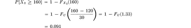
But if the engineer, needing time to carry out the operations, makes a measurement at the earlier time and finds the flow to be x1 = 70 cfs (or lower than the expected values of 100 cfs), then the conditional distribution of X2, the later
Fig. 3.6.3 The marginal and a conditional distribution of X2.
flow, is normal with parameters

Conditional on this new information, the risk of X2 exceeding the critical flow is now
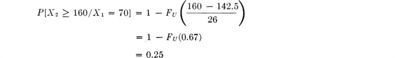
or nearly three times as great as before. If the consequences of failing to open the gates versus those of opening it unnecessarily are of appropriate magnitudes, this change in the high-flow likelihood could alter the engineer’s decision to take action. The marginal and conditional distributions of X2 are plotted in Fig. 3.6.3.
In words, if X1 and X2 are bivariate normal and correlated (positively, say) and if observation of X1 yields an observation greater than the expected (predicted) value m1 it is logical to alter the prediction of X2 upward [Eq. (3.6.23)]. The amount of change should be proportional to the amount X1 deviated from its mean, to the degree of correlation between X2 and X1 and to the relative dispersion of the two variables. The added information contained in the observation of X1 is reflected in a more peaked conditional distribution of X2. This distribution has a smaller variance (σ'2), 2 a reduced mean square error of prediction; the fractional reduction in mean square error is proportional to the square of the correlation coefficient. Perfect correlation (or linear functional dependence: X2 = a + bX1) implies that X2 can be predicted exactly, that is, that the expected squared error in estimating X2 can be completely eliminated by an observation of X1. Complete lack of correlation (or independence in this bivariate normal case) implies that ρ is equal to zero; the predicted value of X2 and the mean square error are left unaltered by the unhelpful information that X1 = x1.
Many of the problems of engineering experimentation and testing can be interpreted in the light of the engineer’s observing one random variable to predict another. Measurements of asphalt content, ultimate compressive stress of concrete, or percentage of optimum compacted soil density are usually made, not because they are of central interest, but because they are easily performed tests on materials properties which are correlated with critical, difficult-to-measure properties such as pavement strength, concrete durability, and embankment stability. The higher the correlation, the better is the test in predicting the adequacy of the key variable.
In this section two important multivariate distributions were considered. The multinomial distribution is a generalization of the binomial distribution. At each of n independent trial, any of k different events might take place.
The multivariate normal (or gaussian) distribution is a generalization of the univariate normal distribution. This commonly applied distribution is extremely tractable. The marginal and conditional distributions, and the distributions of linear combinations of multivariate normal variables, remain normal. In particular the conditional distribution of Y given X = x, when X and Y are bivariate normal, is normal with mean and variance
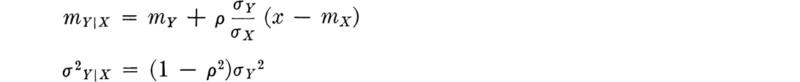
In practice, the assumption of stochastic independence is frequently made. It is a fundamental assumption, for example, in the Bernoulli trials and Poisson-process models studied in Secs. 3.1 and 3.2. In many applications, however, significant dependence exists between the successive trials or years or steps that can be identified in the physical process. This stochastic dependence may be quite general, e.g., the conditional distribution of the amount of rainfall tomorrow may depend in varying degrees on the amounts of rainfall on a number of preceding days. On the other hand, this stochastic dependence may be relatively simple; the conditional distribution of the total rainfall next month may depend only on the amount of rainfall observed this month, but not on that in previous months. This last illustration is an example of Markov dependence, which we shall consider in this section. Initially, in Sec. 3.7.1, we shall make some necessary definitions and consider some examples of simple processes exhibiting the Markov property. In Sec. 3.7.2 we shall treat the simplest case in some detail, and in Sec. 3.7.3, the results for more general models will be introduced and illustrated.
Definition and illustration of the Markov property We want to study phenomena whose probabilistic behavior can be characterized by Markov dependence. The clearest example is the running sum of the number of heads encountered in n independent flips of a coin. Denote this sum by† X(n) for n = 1, 2, . . . . Suppose we have observed the entire history of the coin-flipping process from the first to nth flips, finding X(1) = x1, X(2) = x2, . . ., X(n) = xn. Then the probability that the next value of the process, X(n + 1), will equal any particular value xn + 1, given this entire history, is written in general as

But for this coin-flipping process this conditional probability is equal to simply
The conditional probability is functionally independent of the values of process prior to the present value. The probabilities of how many heads we shall have observed after the next flip depend only on how many we have now, and not by the path by which we got to this present number.
In this simple case, if p is the probability of a head on any flip:
Illustration: Soil testing If a series of compaction tests are being carried out on a particular lift of soil during a large embankment construction, we may assume that each is an independent sample of the material. Record is kept of the number of individual specimens which meet specifications. Let X(n) equal the total number of specimens found satisfactory at the completion of n tests. After four tests, the recorded values were
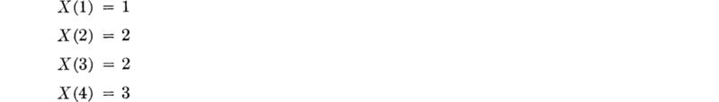
(Clearly, the third specimen was not satisfactory.) The next or fifth specimen will be either satisfactory or not, implying that the value of the process at step 5, that is, X(5), will be either 4 or 3, respectively. The conditional probabilities of these two values of X(5) are p and 1 – p, respectively, p being the probability that any specimen is satisfactory. But this would also be true if the past recorded values had been 0, 1, 2, 3 or 1, 1, 2, 3 or 1, 2, 3, 3, that is, no matter which previous specimen was unsatisfactory. In short, the conditional probabilities of the values X(5) depend only on the fact that the present value, X(4), is 3:

A stochastic process which has the property defined by Eq. (3.7.1) is said to be a Markov process. Such a process is said to be memoryless; the future behavior depends on only its present state and not on its past history.
The Markov property can be appreciated better by considering two non-Markov processes in the coin-flipping phenomenon. Using stochastic-process notation, we can also treat the individual coin flips as a process. Let Y(n) = outcome of the nth flip (= 0 or 1 for tail or head, say). This Bernoulli process has no trial-to-trial dependence:
As discussed, the total-number-of-heads process X(n) has the one-step or Markov dependence defined in Eq. (3.7.1). Still other processes associated with coin flipping can be defined which depend on a part or the entire past history of the process. For example, define Z(n) = number of heads in the last two tosses. In this case, the probability of the next, or (n + l)th, value of the process is influenced by more than just the present, or nth, value of the process. For example, in both of the following cases the nth value of the process is 1, but the probability of the next value being 1 depends on what the value was at step n – 1:
Here knowledge of the previous, (n – l)th, value (or state) of the process permits one to deduce that in the first case, the nth flip was a head, while in the second case the nth flip was a tail. This information in turn influences the probability that Z(n + 1) will equal 1. The Markov property [Eq. (3.7.1)] does not hold in this case, and so the process Z(n) is not a Markov process.
Typical observed “time” histories of these three stochastic processes, X(t), Y(t), and Z(t), are shown in Fig. 3.7.1. These observations are called sample functions or realizations of the process.
The word “state” is frequently and conveniently used in discussing Markov processes. If the total number of heads is five at the eighth flip, i.e., if X(8) = 5, it would be said that the process is in “state” 5 at “time” 8. Although the set of possible states (i.e., the sample space) can be either continuous or discrete, we shall restrict our attention to discrete-state processes, called Markov chains (or random walks). In this case it is possible to index or number the states, typically 0, 1, 2, . . ., to a finite or infinite number. Therefore we shall usually write a statement such as P[X(n) = i] rather than P[X(n) = x] and read “the probability that the process is ‘in state i’ at step (or ‘time’) n, ” rather than “the probability that the value of the process at step n is x.”
Examples Engineering processes which have been or might be modeled as Markov processes are common. Some examples are:
1. The total number of subway system users with destination station B, which have entered at station A, observed each 1 min from 5:30 P.M. to 5:45 P.M.
2. The number of vehicles waiting in a toll-booth queue, the process being observed (not at fixed intervals of time but) just after a car either enters the queue or leaves the toll booth.
3. The state of deterioration of the wearing surface of a bridge (e.g., state 0 = smooth; state 1 = fair; state 2 = rough; state 3 = unacceptable) observed each year after its placement.
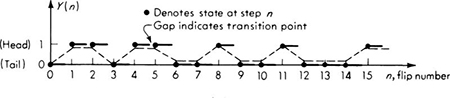
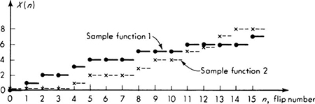
Fig. 3.7.1 Typical sample functions from coin tossing, (a) A typical function of Y(n), the outcome of the nth flip; note the different ways of sketching the sample functions. (b) Two typical sample functions of the process X(n), the total number of heads at the nth flip; sample function 1 corresponds to observations shown in (a). (c) A typical sample function of the process Z(n), the number of heads in previous two flips; function corresponds to Y(n) observation in (a). Define Z(n) = X(n) for n = 0 and n = 1.
Note that in the last case, the states are not naturally quantitative, the state numbers simply index the various states. Typical sample functions of these three processes might appear as shown in Fig. 3.7.2.
If truly continuous-state spaces are approximated by a discrete set of states, still other examples are possible: the amount of water in a dam observed each month after the inflows and releases for the month have occurred, or the total distance downstream that a particular sediment particle has moved after n impacts by other particles.
The Markov property In each application one must ask if the Markov property [Eq. (3.7.1)] is a reasonable assumption. In words, does the future behavior depend only on the present state, and not on the past states? Considering some of the illustrations above, for example, the process of total passengers will be Markov if the numbers arriving in each minute are mutually independent; the bridge-surface-condition process has the Markov property if, roughly, the “damage rate” depends only on the present degree of damage and possibly the age n, but not on, for example, how long the surface spent in state 1; and the dam-contents process will be Markov if, for instance, the monthly flows are independent and the amount of water released depends on the contents (and possibly the date n). In the last case, the process would not be Markov if there were correlation between monthly inflows. Positive correlation would mean that low flows are likely to follow low flows. This correlation would imply that the low dam contents this month are more likely to be followed by low contents next month if the contents were also low last month than if they were not. This is a dependence on the past which is inconsistent with the Markov property. Like independence, the Markov assumption must in practice be made in the basis of professional judgment. The advantage of adopting the assumption is its relative analytical simplicity.

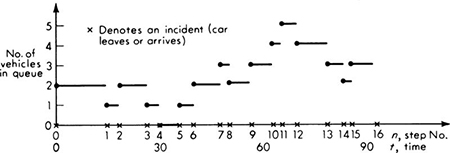
Fig. 3.7.2 Typical sample functions of processes that can be modeled as Markov chains, (a) A typical sample function of a passenger-arriving process; note that average rate of arrival may depend on time, (b) A typical sample function of a toll-booth queue; note that the discrete steps occur at random times, (c) Two typical sample functions of a bridge-wearing-surface process; note that the process may remain in the same state for two or more steps.
Typical questions We shall be interested in asking a number of kinds of questions about Markov chains. For example, what is the probability that the process is in state i at time n? The reader should immediately know the answer to this question in the case of the total-number-of-heads process X(n) (see Sec. 3.1.2). Or given that the process (e.g., the dam) is now in state i (e.g., half full), we might ask what is the probability that k steps (e.g., months) from now it will be in state j (e.g., full)? Symbolically, calling the present time n, we seek
We might also ask, when appropriate, what is the average fraction of the steps (e.g., average proportion of the time) that the process (e.g., the toll-booth queue) spends in state i (e.g., empty). Of the bridge-wearing surface-deterioration process, we might ask what is the probability distribution of the time to the unacceptable state (i.e., the time to “first passage” into state 3)?
Parameters To describe the probabilistic behavior of a Markov chain, we need to have two sets of information. These represent the parameters of the process.
1. First, we must know the state in which the system originates at “time” 0, or, more generally, a distribution on the initial states:
Note the introduction of a shorthand notation qi(n) for the probability that the process is in state i at time (or step) n, in general:
2. Second, we need the transition probabilities Pij (n). Each of these is the probability that the process will be in state j at time n given that it was in state i at the previous step:
In different words, the transition probability Pij(n) is the probability that the process will “jump” into state j at the nth step if it is in state i at the (n – l)th step. In general this probability is a function of “time” or the step number n. If not, the process is said to be “homogeneous” in time, in which case we write simply
In the previous examples, we can discern immediately some characteristics of their initial-state probabilities qi(0) and transition probabilities Pij(n). For example, the total-number-of-passengers process starts with certainty in state 0, by definition, and its transition probabilities are such that Pij(n) = 0 for j < i, since the process is a cumulative one. The transition probabilities could be calculated if the distribution of number of passengers arriving in each minute were known. This might be the same for all minutes over the 15-min interval of interest, implying that the chain is homogeneous, i.e., that the pij (n) are independent of time pij.
The process describing the number of vehicles waiting in a toll queue, on the other hand, might start in most any state. The transition probabilities are restricted to permitting jumps to the next lower or next higher state only, since a transition occurs only when a vehicle is added or subtracted from the queue. Transitions to other states have zero probability. Again it might be reasonable to assume that the transition probabilities are time-independent. It can be shown, for example, that, if the vehicle arrivals follow a Poisson processes with arrival rate λ, and if the service time taken at the toll booth is exponentially distributed with mean 1/μ (i.e., the mean service rate is μ), then the queuing process is Markov† with transition probabilities dependent in a simple and intuitive manner on these “rates” (Parzen [1962]):
A bridge-surface deterioration process with four states (0, 1, 2, 3) denoting advancing states of deterioration would probably start in state 0 at the time of opening of a new surface. In any year the surface condition could potentially advance to any of the higher numbered states of deterioration, or it might remain as it was. It must remain in the final state. † The implication is that p33 (n) = 1. Such a state (i.e., with pii (n) = 1 for all n) is said to be a trapping state, since once there the process cannot leave it. Since the bridge surface cannot improve, the process can never make a transition to a lower state, for example, p21 (n) = 0 for all n. The values of the other transition probabilities could presumably be estimated from maintenance-department records, depending on the type of surface and type of traffic conditions. If absolute age of the material were influential, the probabilities Pij (n) would depend on n and a complete set of 4 × 4 = 16 transition probasbilities would be needed for each time n.
Transition-probability matrix Transition probabilities are conveniently displayed in square arrays or matrices, which we denote II (n) (or simply II for homogeneous chains). For example, in the second year, n = 2, the transition probabilities for the bridge surface would appear as:
For example p00 (2) is the probability of remaining in state 0 during the second year given that in the previous year the state is 0, and poi(2) is the probability of a transition leaving state 0 and entering state 1 in the second year, given that it is in state 0 in year 1. Since the surface cannot improve, p10 (2) = 0, the probability of a transition from state 1 to state 0 in the second year is zero. This accounts for all the zero elements. For the trapping state, p33 (2) = 1 because the pavement can only remain in state 3. The state number designations on the margins of the matrix will usually be omitted.
In the case of the toll-booth queue the array of (homogeneous) transition probabilities would have this structure:
Recall that a transition takes place when a new car arrives or an existing car is serviced. This matrix is constructed by noting that if zero cars are in the queue, the only possible transition is for a car to arrive: p00 = 0 and p01 = 1. With one vehicle in the queue the probability of its being serviced and the queue length becoming zero is p, i.e., p10 = p. The only other possible event involves the addition of a vehicle to the queue. Thus pu = 1 – p, since p10 and p12 describe the only events that can occur at a transition. Note again that the transitions do not take place at fixed time spacings but at random times with the addition or subtraction of a vehicle from the queue. Note too that in this case there is no logical upper limit to the set of states. Such a process is called an infinite chain.
Since at each step any Markov process must either remain in the same state or make a transition to some other state, and since these are mutually exclusive events, it is obvious that the sum of the probabilities in any row of the array of transition probabilities must equal unity. We can use this observation to calculate one of the elements in a row if all the others are known. This was done in the preceding example.
In the next section we shall demonstrate typical calculations on Markov chains using the simplest possible example, that is, a two-state homogeneous chain. In Sec. 3.7.3 we shall see more general results and illustrations.
The simplest example of a Markov chain is one which has but two states, 0 and 1, and one which is homogeneous, i.e., its transition probabilities Pij are independent of time. This case will serve to introduce the analysis of Markov chains, while keeping the algebra simple. The illustration is one of a system with random demand, both the existence and the duration of the demand being probabilistic.
We shall consider the occupancy history of a “slot” in a transit system proposed for congested central cities. In the proposal, a continuous moving “belt” of “slots” (each slot designed for a single passenger) passes along the transit route. The route has a large number of stations or stops, at two- or three-block intervals. At these stations each individual slot or compartment slows down. If it is full, its passenger may exit if he wishes; if the slot enters the station empty or becomes empty, a waiting user, if any is present, will fill it. We want to follow the history of a single, particular slot as it passes from station to station.
The process X(n), n = 0, 1, 2, . . ., will take on value 0 or 1 at step n depending on whether the slot is empty or occupied between the nth station and the (n + l)th station; that is, the slot is “observed” after it leaves station n.
The transition probabilities can be calculated from the following assumptions. At any station there is a probability p that one or more persons will be waiting to use the slot if it is empty. For simplicity (i.e., to make the process homogeneous) we assume that this probability is the same at all stations. Again for simplicity we shall assume that if there is an individual in the slot as it enters the station, he will get off with probability p', independently of when he got on, and independently of whether another user is waiting.
Under these independence assumptions about the transit users7 behavior, the process X(n) is a Markov process. The Markov condition, Eq. (3.7.1), is satisfied, since, in words, the probability that the slot will be full, say, as it leaves the next station depends upon whether it is full or empty as it leaves the present station, but not on the history of how it got to its present condition, †
The parameters of the process are:
1. Initial-state probabilities:
For illustration, we assume arbitrarily that the slot starts out empty (i.e., it is empty when entering station 1) with certainty; that is,
2. Transition probabilities:
(a) If the car leaves a station empty, it will leave the next full only if a passenger is waiting there. Therefore:
and, since p01 plus p00 must equal 1,
(b) If the car leaves one station full, it will leave the next empty only if that passenger gets off and none is waiting. This event happens wdth probability p′(1 – p). Calling this product r, we
The transition-probability matrix is
The marginal probabilities of state We seek first the probability that the process will be in any state i at any time n. For example, we might want the probability that the slot is full on leaving the second station. We find the probability
by working frontward one step at a time. For example, to find qi(2), consider first that
The first equation says, in words, that the probability that the process is in state 1 at time 1 is the probability that it was in state 1 at the previous step and stayed there plus the probability that it was previously in state 0 and then it jumped to state 1. Knowing these probabilities for step 1, we can find q1(2), since, by the same argument,
![]()
Then, substituting, we obtain
Each term represents a path by which the process might have ended up in state 1 at time 2. The third term, for example, is the probability that the slot, say, was initially full, then empty, and then full again.
For the case of a two-state homogeneous chain, one can show by induction that for any† n:
The probability of being in state 0 at step n or q0 (n) is, of course, just 1 – q1(n). For example, in our case, the probability that the slot will be full after n stations is
If r = 0.4 and p = 0.5, then the probability that the slot will be empty as it leaves station 4 (given, recall, the initial condition that it entered station 1 empty) is
This result accounts, of course, for all the possible sequences of empty and full conditions that start empty and end up empty on leaving station 4.
The m-step transition probabilities More generally we might seek the probability that the process will be in state j m steps later given that it is in state i at time n. For example, we might ask, given that the slot was full on leaving station 8, what is the probability that it will be full two stations later, i.e., after station 10. These are called m-step transition probabilities pij(m); the simple transition probability pij represents the m = 1 or one-step case. In general,
Owing to the homogeneity in “time” of the process, the argument used above for a start from the initial state still holds, now translated n steps in time. Now, too, we are given that the process is with certainty in a specific state at time n. Therefore, for n = 8, m = 2, i = 0, and j = 1, the two-step transition probability p01(2) can be found from Eq. (3.7.23), letting q1(0) = 0 and q0(0) = 1:
![]()
This is a result we could also arrive at by a simple direct argument, since each term represents a path by which the process starts empty at step n and ends up full two steps later.
To generalize to any m we can make use of Eq. (3.7.24) in a similar way and conclude that the m-step transition probabilities are, given a start in state 1 at time n:
and, given a start in state zero at time n,
The other two m-step transition probabilities, p10(m) and p01(m), are simply 1 – p11(m) and 1 – p00(m).
For example, if we ask for the probability that a slot will be empty four stations after leaving station n empty, we ask for
![]()
If p = 0.5 and r = 0.4,
This is, of course, exactly equal to q0(4) [Eq. (3.7.26)], since we assumed there that the initial state was empty, and since the m-step transition probabilities are independent of the time n for homogeneous Markov chains.
Steady-state probabilities In many cases the initial state probabilities are not well known, and it is meaningful to ask, “Do the probabilities of state qi(n) take on values which are independent of the initial state?” Can one give the probability that a slot will be full at some future time without knowing whether it was initially full or empty? In different words, does the process reach a probabilistic steady-state or equilibrium condition, and is this condition independent of its starting position? Here, steady state does not suggest that the process is fixed in a given state, but rather that it is moving (stochastically) among the states in a manner which is uninfluenced by “starting transients.” The obvious analogy is with the dynamic response of simple deterministic mechanical systems to periodic forcing functions.
The answer to these questions for the simple homogeneous chain we are considering is affirmative. Notice that as n grows in Eq. (3.7.24) for q1 (n), the first term grows smaller and smaller in absolute value, † leaving only the second term:
and
These results are independent of the initial-state probabilities and of the time n. The heuristic interpretation of the first result is that the probability that the process is in state 1 at any time (after the process has been going for some time) is equal to the ratio of the “rate” at which the process enters the state (p01) compared to the total rate at which the process enters all states (p01 + p10).
These long-run or steady-state probabilities will be denoted![]() . Formally, they are the limits
. Formally, they are the limits
The probability ![]() can be interpreted as either:
can be interpreted as either:
1. The probability that the process will be in state i at any point in time (a sufficiently long time after the process starts), or
2. The average fraction † of the time (i.e., the average fraction of the number of steps) that the process is in state i.
In our illustration, the steady-state probabilities are
With specific numerical values for p and r, we can study the rate at which the transit system process leaves the transient initial-state-dependent condition and approaches the steady-state condition. For example, for r = 0.4 and p = 0.5 the following values for q0(n) are obtained, depending on whether the slot begins in the empty or full state:
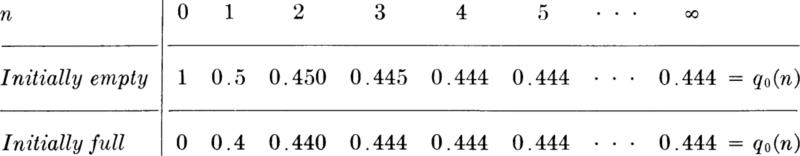
No matter what the initial state, the probability of being empty is r/(p + r) = 0.444 within four stations. If the probability of a passenger’s getting off is smaller, say r = 0.18, and if the probability of a passenger’s waiting is smaller, say p = 0.3, then the state condition is approached more slowly †:
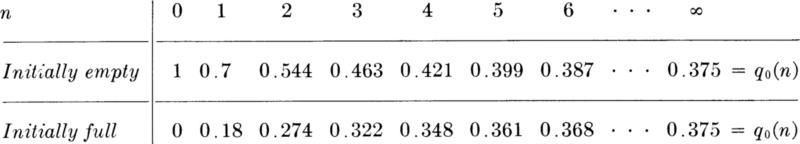
Convergence is slower, but eventually the probability of the slot being empty is r/(p + r) = 0.375, no matter whether it was initially empty or full.
We interpret this last result, ![]() , as either the probability that the slot will be empty on leaving any particular station or as the average number of stations from which the slot will depart empty.
, as either the probability that the slot will be empty on leaving any particular station or as the average number of stations from which the slot will depart empty.