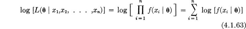
A probabilistic model remains an abstraction until it has been related to observations of the physical phenomenon. These data yield numerical estimates of the model’s parameters, and provide an opportunity to verify the model by comparing the observations against model predictions. The former process is called estimation; it is the subject of Sec. 4.1. The latter, comparative, process includes verification of the entire model (Sec. 4.4), but more broadly it includes the search for significance in a batch of statistical data. Conventional methods of significance testing are discussed in Sec. 4.2.
Consider the engineer who has developed a model of some physical phenomenon leading to a proposed functional form (e.g., lognormal) of the governing probability distribution. He must next estimate its parameters and then judge the validity of the model. Both these processes, estimation and verification, require data for the resolution. Repeated experiments will yield a sample of observed values of the random variable, say n in number. The resulting set of n numbers might be treated by the data-reduction techniques discussed in Chap. 1, yielding sample moments and a histogram. If we were to repeat the sequence of n tests, it is the nature of the probabilistic phenomenon that we would get (except coincidentally) a different set of values for the n numbers and therefore for the sample moments and histograms. Any reasonable rule for extracting parameter estimates from such sequences of numbers (e.g., a rule which says “estimate the parameter m by the average of the sample”) would consequently yield different estimates of the values of the model’s parameters. No single sequence of observations finite in number can be expected to give us exact model parameter values, because the data itself is a product of the “randomness” which characterizes the phenomenon. We must be prepared then to accept a data-derived parameter value as no more than an estimate of the true value, subject to an error of uncertain but, as we shall see, not unquantifiable magnitude.
We can also use data to evaluate the validity of an hypothesized model by comparing the model’s predictions with observed occurrences. The relative frequency of particular events, for example, can be measured in the experiment and compared with probabilities computed from the model. Consistent and large discrepancies between such numbers would cast doubt on the ability of the hypothesized model to describe the physical phenomenon, while close correspondence would tend to lend credence to the proposed model. A moment’s reflection, however, will reveal that, again owing to the probabilistic nature of the situation, one can seldom state that certain observed data are sufficient to reject or accept categorically a proposed model. An apparent discrepancy between model and reality may simply be the result of the occurrence in that particular data of a relatively rare but not impossible set of events. On the other hand, there may be a number of other models capable of yielding (with small or large likelihood) a set of observed data judged to be in accordance with our model’s predictions. Consequently such evaluations will have to be qualified and phrased in a way that reflects the possibilities of such errors in the conclusions.
In short, if parameter estimation and model verification are based on practical sample sizes, there will remain uncertainty in the parameter values and perhaps uncertainty in the validity of the model itself. We recognize, then, that the engineer faces at least three distinct types of uncertainty. The first is the natural, intrinsic, irreducible, or fundamental uncertainty of the probabilistic phenomenon itself. This was emphasized in previous chapters. The second type of uncertainty can be called statistical. It is associated with failure to estimate the model parameters with precision. It is not fundamental, in that it can be virtually eliminated at the expense of a very large sample size. The third kind of uncertainty, that in the form of the model itself (the model uncertainty), can, in principle, also be eliminated with sufficient data. For example, a Bernoulli trial model says the number of heads in k flips of an unbalanced coin is a binomial random variable B(k,p). The outcome of any experiment (of k flips) is fundamentally uncertain, even given the validity of the binomial distribution and given a known value of p. With only a limited number of experiments upon which to base an estimate, however, the true value of p will remain in some doubt, i.e., subject to statistical uncertainty. A limited amount of data will not provide enough comparisons between histograms and the binomial PMF to guarantee that the model holds (e.g., there may not be independence among the flips); model uncertainty remains. More data will tend to reduce the magnitude of statistical and model uncertainty. The fundamental uncertainty remains unchanged by the number of past experiments.
This chapter represents a small but appropriate sampling of applied statistics† a widely studied and broadly applied discipline dealing with the relationships among abstract probabilistic models and real data gathered from situations in engineering, industry, and the sciences. We shall see that convenient conventions have been established for reporting and discussing the very difficult questions surrounding the second and third kinds of uncertainty, those associated with estimation and model verification.
Having hypothesized the type or functional form of his model, the engineer’s first problem upon being confronted with numerical data is the estimation of the values of the parameters of these functions. In this operation he chooses the parameters’ estimates so that the model, in some sense, best fits the observed behavior. We seek estimators (certain functions of the random variables in the sample) which promise this fit, and then we study the nature of these estimators as random variables.
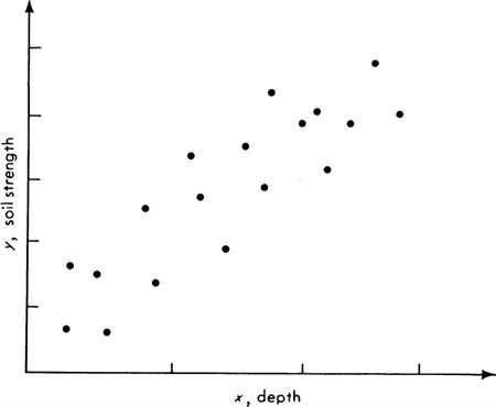
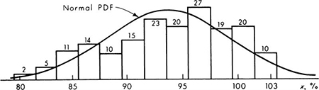
We choose to introduce this topic through illustrations. A structural engineer concerned with strength of reinforced-concrete structures needs information concerning the force at which the tensile reinforcement will yield. A yield-strength theory for ductile steel argues that a bar yields only when its many individual “fibers” have all yielded, and, since each such fiber contributes in an additive manner to the total force, it should be expected that X, the yield force of a bar, would be normally distributed†:
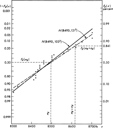
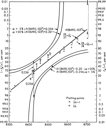
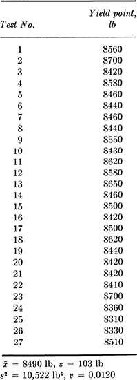
The engineer tests a number of specimens of no. 4 (nominally ![]() in diameter) mild steel reinforcing bars. The data from 27 specimens are shown in Table 4.1.1. The sample mean
in diameter) mild steel reinforcing bars. The data from 27 specimens are shown in Table 4.1.1. The sample mean ![]() and sample standard deviation s (Sec. 1.2), are 8490 and 103 lb, respectively.† Accepting the conjecture that the yield force of such a bar has a normal distribution, what values of the parameters m and σ should be used when describing the behavior of a no. 4 reinforcing bar in this lot?
and sample standard deviation s (Sec. 1.2), are 8490 and 103 lb, respectively.† Accepting the conjecture that the yield force of such a bar has a normal distribution, what values of the parameters m and σ should be used when describing the behavior of a no. 4 reinforcing bar in this lot?
Table 4.1.1 Tests of no. 4 rein forcing bars from a single lot
It would be contrary to the engineer’s common sense to consider estimates of m and σ which differ much, if any, from the sample statistics ![]() and s. The moments of the numerical data provide obvious and reasonable estimates of the corresponding moments of the proposed mathematical model.
and s. The moments of the numerical data provide obvious and reasonable estimates of the corresponding moments of the proposed mathematical model.
This intuitively satisfactory rule for calculating model parameter estimates from data is given the name the method of moments. It says that the estimator ![]() of mX should be the sample mean, and the estimator
of mX should be the sample mean, and the estimator ![]() of the variance σ2 is the sample variance. Similar rules hold for higher moments of the variable and the data, although these two estimators are sufficient for two-parameter distributions.
of the variance σ2 is the sample variance. Similar rules hold for higher moments of the variable and the data, although these two estimators are sufficient for two-parameter distributions.
In the example, the estimators (rules) lead to the following estimates (values) ‡ of the mean and variance
Given these parameter values the engineer can define completely his model [Eq. (4.1.1)] of the bar-force random variable and he is prepared to make such statements as “The probability is 5 percent that the yield force of any particular bar will be less than m – 1.65σ = 8490 – 1.65(103) = 8490 – 173 = 8317 lb.”
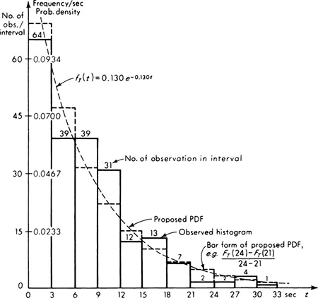
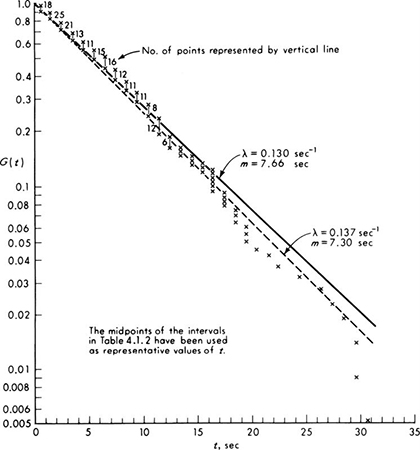
Illustration: Exponential distribution It is not always true, of course, that the parameters of a distribution are equivalent to moments. The parameters n and p of the binomial distribution (Sec. 3.1.3) are examples. The moments are, however, functions of the parameters, and these equations can normally be solved to yield the parameters in terms of the moments.§ Consider the following simple example. A traffic engineer who had adopted the common assumption of Poisson traffic (Sec. 3.2) measured the gap or time-between-successive-cars data shown in Table 4.1.2. The sample mean of this data is 7.66 sec. The mathematical model states that this distribution is exponential with parameter λ:
Table 4.1.2 Observed gaps in traffic: Arroyo Seco Freeway (Los Angeles) *
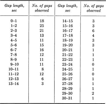
Interval midpoint is used as value of ti; Σxi = 1640; total no. of observations = 214; ![]() sec; Σti2 = 21,396 sec2.
sec; Σti2 = 21,396 sec2.
* Source: Gerlough [1955].
The mean of this distribution is (Sec. 3.2.2)
Hence the parameter, as a function of the moments, is simply
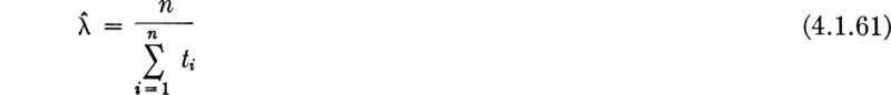
By the method of moments [Eq.(4.1.2)] the estimator of mT is the sample mean. The corresponding estimator of the parameter is the reciprocal of the sample mean. For this data the estimate of λ is
Adopting this parameter value, the engineer now can state, for example, that the probability of a gap length of 8 to 10 sec is

The sample moments have been proposed as reasonable estimators of the moments of the mathematical model. The sample moments, it should be remembered, were proposed in Chap. 1 only as logical numbers to summarize a batch of numbers observed in some physical experiment. They were given definitions [Eqs. (4.1.2) and (4.1.3)] in terms of those observed numbers, x1 x2, . . ., xn. The moments m and σ2, on the other hand, are constants. They are parameters of some distribution defining the behavior of a random variable X, which is a purely mathematical model. Once we have adopted the assumption, however, that this mathematical model is controlling the physical experiment, we can interpret the xi’s as observed values of a random variable X. In this new light, the sample average ![]() is the numerical average of n observations of the random variable X.
is the numerical average of n observations of the random variable X.
Sample statistics as random variables With the ultimate goal of gaining some knowledge of how good an estimator of the mean m the sample average ![]() is, let us back up one step to a point before the physical experiments have been carried out, i.e., to a point before the observed values x1, x2, . . ., xn are known, and then let us see what can be said about this sample mean. Define the random variables X1, X2, . . ., Xn as the first, second, . . ., nth outcomes of the sequence of n experiments involved in the process† of sampling. Each Xi has the same distribution as X, sometimes called in this context the population to be sampled. In particular, each variable has mean and variance equal to the population mean mX and population variation σX2. Then the sample mean which we intend to compute can be written
is, let us back up one step to a point before the physical experiments have been carried out, i.e., to a point before the observed values x1, x2, . . ., xn are known, and then let us see what can be said about this sample mean. Define the random variables X1, X2, . . ., Xn as the first, second, . . ., nth outcomes of the sequence of n experiments involved in the process† of sampling. Each Xi has the same distribution as X, sometimes called in this context the population to be sampled. In particular, each variable has mean and variance equal to the population mean mX and population variation σX2. Then the sample mean which we intend to compute can be written
and the sample variance is
Capital letters are now used for the sample mean and the sample variance to emphasize the fact that, as functions of the random variables X1, X2, . . ., Xn, these sample averages are themselves random variables. After the experiments, the outcomes X1 = x1, X2 = x2, . . ., Xn = xn will be recorded, and the observed values ![]() and s2 of the random variables
and s2 of the random variables ![]() and S2 will be computed. Functions g(X1X2, . . ., Xn) of a sample X1 X2, . . ., Xn are called sample statistics. The sample mean and sample variance are just two of many such sample statistics of potential interest. Others include X(n) = max [X1X2, . . ., Xn], the largest observed value, and X(i), the ith smallest value in the sample. (The latter is called an “order statistic.” See Prob. 3.46.) Our present interest in sample statistics is due to their role as estimators of unknown parameters.
and S2 will be computed. Functions g(X1X2, . . ., Xn) of a sample X1 X2, . . ., Xn are called sample statistics. The sample mean and sample variance are just two of many such sample statistics of potential interest. Others include X(n) = max [X1X2, . . ., Xn], the largest observed value, and X(i), the ith smallest value in the sample. (The latter is called an “order statistic.” See Prob. 3.46.) Our present interest in sample statistics is due to their role as estimators of unknown parameters.
Moments of the sample mean ![]() As a random variable, the sample mean,
As a random variable, the sample mean, ![]() is open to study of such questions as, “What is its average value?” “What is its variance?” and “What is its distribution?” In particular, since we use
is open to study of such questions as, “What is its average value?” “What is its variance?” and “What is its distribution?” In particular, since we use ![]() as its estimator, what is the relationship between answers to these questions and the mean mX of the random variable X? In this section we concentrate only on first- and second-order moments of this estimator. The moments of
as its estimator, what is the relationship between answers to these questions and the mean mX of the random variable X? In this section we concentrate only on first- and second-order moments of this estimator. The moments of ![]() are independent of the form of the distribution of X and they are sufficient to answer many questions about estimators. To go further we will have to specify the PDF of X. Do not forget that we study
are independent of the form of the distribution of X and they are sufficient to answer many questions about estimators. To go further we will have to specify the PDF of X. Do not forget that we study ![]() only because we ultimately intend to use observations of
only because we ultimately intend to use observations of ![]() to estimate an unknown mX.
to estimate an unknown mX.
Consider first, then, the mean of the sample mean [Eq. (4.1.8)]:
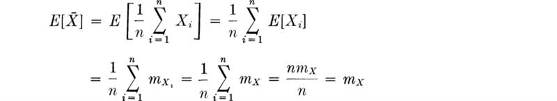
In short,
In words, the expected value of the sample mean is equal to the mean of the underlying random variable. Any other answer would undoubtedly leave us somewhat uneasy as to the merit of ![]() as an estimator of mX.
as an estimator of mX.
As a random variable it cannot be expected, however, that ![]() will often, if ever, take on values exactly equal to the mean and hence give a perfect estimate of mX. The estimation error,
will often, if ever, take on values exactly equal to the mean and hence give a perfect estimate of mX. The estimation error, ![]() is a random variable with a mean of zero. A measure of the average magnitude of the random error associated with an estimator can be gained through the expected value of its square (called the mean square error). This second- order moment reduces in this case to the variance of
is a random variable with a mean of zero. A measure of the average magnitude of the random error associated with an estimator can be gained through the expected value of its square (called the mean square error). This second- order moment reduces in this case to the variance of ![]() :
:
The next question is then how Var ![]() depends on Var
depends on Var![]() :
:
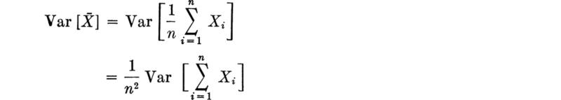
Using Eq. (2.4.81b) for the variance of a sum of random variables,
We shall restrict our attention to those cases where the sampling of X is carried on in such a manner that it may be assumed that the individual observations X1 X2, . . ., Xn are mutually independent random variables. Such sampling is called random sampling. The main reason for this restriction is simply that, even if the stochastic dependence involved lent itself to description, nonindependent types of sampling are usually more difficult to analyze. †
It should be pointed out that in practice it is virtually impossible to ascertain that true random sampling is being achieved, but, if the engineer wishes to exploit the theory of statistics to give him a quantifiable measure of the errors in estimation, it remains necessary that he take precautions to insure that there is little systematic variation or “persistence” from experiment to experiment. In sampling a population of reinforcing bars, for example, one would avoid taking more than one specimen from any one bar because correlation among specimens within a bar is to be expected.
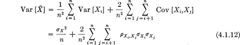
An immediate consequence of assumption of random sampling is the great simplification of Eq. (4.1.12). For independent samples, the correlations are zero and
The simplicity of these formulas belies their great practical significance. We now have a measure of the expected error associated with the rule that states that mX should be estimated by![]() . No matter what the distributions of X and
. No matter what the distributions of X and ![]() , through Chebyshev’s inequality [Eq. (2.4.11)] we are now in a position to make probability statements regarding the likelihood that the estimator
, through Chebyshev’s inequality [Eq. (2.4.11)] we are now in a position to make probability statements regarding the likelihood that the estimator ![]() will be within certain limits about mX, say
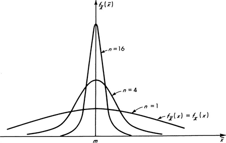
will be within certain limits about mX, say ![]() Equation (4.1.14) also shows how, for fixed probability (or fixed k), the width of these limits decreases as the sample size increases. Notice, for example, that to halve the interval width from that associated a single observation (n = 1) of X, one must increase the sample size to n = 4. To halve it again, n must equal 16, and so forth. The distributions of
Equation (4.1.14) also shows how, for fixed probability (or fixed k), the width of these limits decreases as the sample size increases. Notice, for example, that to halve the interval width from that associated a single observation (n = 1) of X, one must increase the sample size to n = 4. To halve it again, n must equal 16, and so forth. The distributions of ![]() for these cases are sketched in Fig. 4.1.1. It becomes increasingly expensive to continue to reduce the magnitude of
for these cases are sketched in Fig. 4.1.1. It becomes increasingly expensive to continue to reduce the magnitude of![]() , the measure of error in the estimator
, the measure of error in the estimator![]() . It should be remembered, however, that
. It should be remembered, however, that ![]() is a measure of expected error. In a state of ignorance regarding the true mean we can only say that the sample averages based on larger n are more likely to fall closer to mX than those derived from less information.
is a measure of expected error. In a state of ignorance regarding the true mean we can only say that the sample averages based on larger n are more likely to fall closer to mX than those derived from less information.
Fig. 4.1.1 Distribution of ![]() for n = 1, 4, 16.
for n = 1, 4, 16.
Moments of the sample variance; bias A brief, similar study of the first- and second-order moment behavior of the (random variable) sample variance S2 will lead us to some additional conclusions. We are interested in S2 because we have proposed using S2 as an estimator of the parameter σ2. By definition,
Expanding the square and taking expectations leads directly to the conclusion that (for random samples)
The striking and somewhat disturbing conclusion is that the expected value of the second central moment of the sample E[S2] is not equal to the second central moment of the probability distribution σ2. On the average over many different samples, S2 will not equal the parameter σX2 for which it has been proposed to serve as an estimator, but will equal something smaller.†
Estimators, like S2, whose expected values are not equal to the parameter they estimate are said to be biased estimators. On the assumption that bias is an undesirable property, one can easily determine an unbiased estimator of the variance.
The estimator S2*, which we define as
or
is a sample statistic whose expected value is n/(n ‒ 1) times the expected value of S2 or
Hence S2* is an unbiased estimator of σX2. For this reason the formulas
are found in many texts discussing data reduction in place of Eqs. (1.2.2a) and (1.2.2b) for s2. However, without the formal mechanism of probability and statistics and without the number of assumptions (e.g., independence and desirability of an unbiased estimator) which led us to Eq. (4.1.19), there is no theoretical reason to favor s2* over the more natural s2 as a numerical summary of a batch of numbers.
In the bar-yield-force illustration, the estimator S2 led to an estimate of (103)2 for σ2, and the unbiased estimator S2* yields an estimate of (105)2.
Even if S2* is unbiased, however, it is not necessarily true that S2* is a “better” estimator of σ2 than S2. In general, the error between any (biased or unbiased) estimator ![]() and the parameter it estimates θ is
and the parameter it estimates θ is![]() . (The former value is random; the second is a constant.) The mean square error
. (The former value is random; the second is a constant.) The mean square error ![]() is found easily upon expanding the square to equal
is found easily upon expanding the square to equal
which depends on both the variance and the bias, ![]() , of the estimator. Therefore, the mean square errors of the two estimators S2 and S2* are
, of the estimator. Therefore, the mean square errors of the two estimators S2 and S2* are
and
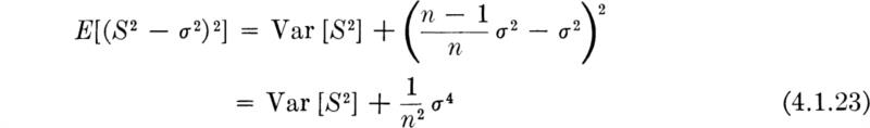
It is not immediately clear which estimator has the smaller mean square error. For a special case, that where X is normally distributed, some simple algebra will show that †
Substituting into the previous two equations for the mean square errors, we can calculate the ratio q(n) of the expected squared error of S2 to that of S2*:
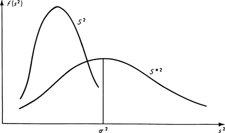
The ratio is less than 1 for all values of n. For example, ![]() . In other words, although S2 has an expected value different from σ2, the expected value of its squared error is smaller than that of the unbiased estimator S2*. The latter estimator leads more frequently to larger errors. This condition is sketched in Fig. 4.1.2 for small n where it is most extreme. In customary statistical terminology, although unbiased, S2* is not a minimum-mean-square-error estimator† of σ2.
. In other words, although S2 has an expected value different from σ2, the expected value of its squared error is smaller than that of the unbiased estimator S2*. The latter estimator leads more frequently to larger errors. This condition is sketched in Fig. 4.1.2 for small n where it is most extreme. In customary statistical terminology, although unbiased, S2* is not a minimum-mean-square-error estimator† of σ2.
Choice of estimator One can conclude generally that the choice of the sample statistic (the function of the observed values) which he should use to estimate a parameter is not necessarily obvious. Any reasonable statistic can be considered as a contending estimator. The sample median, sample mode, or even the average of the maximum and minimum value in the sample are not unreasonable estimators of the mean of many distributions. The method of moments is one general rule for selecting estimators. The method of maximum likelihood (Sec. 4.1.4) is yet another, very common general rule. The question of choosing the
Fig. 4.1.2 Comparison of distributions of S2 and S2*, an extreme case.
best estimator is ambiguous until “best” is defined. Such intuitively desirable properties† of an estimator as its being unbiased and as its being the estimator which promises the minimum mean square error are unfortunately not necessarily combined in the same sample statistic, as was seen in comparing S2 and S2* as contending estimators of σ2. The search for and study of “best” or just “good” estimators is one of the tasks of mathematical statisticians. We refrain from venturing further into the questions of defining other desirable properties, or of choosing among contending estimators. In Sec. 4.1.4 we present an alternative general method, the method of maximum likelihood. It is an intuitively appealing method of choosing estimators which are, on the whole, equal to or better (in the mean-square-error sense) than those estimators suggested by the method of moments.
We have seen that a sample statistics mean and variance, which we were able to find without reference to the distribution of X, are sufficient to describe the salient characteristics of the statistic as an estimator of a model parameter. They define its central tendency relative to the parameter and its dispersion (mean square error) about the true parameter; in particular they indicate the dependence of this latter factor on sample size. More precise, quantitative statements of the uncertainty in parameter values are possible if the entire distribution of the sample statistic is utilized. (This distribution depends upon the distribution of X.) We shall find that one vehicle for such statements is the confidence interval.
The distribution of a sample statistic, which is a function of the random variables X1, X2, . . ., Xn in the sample, depends upon their (common) distribution. The methods of derived distributions (Sec. 2.3) are in general necessary to determine the distribution of the statistic. ‡ We shall focus our attention here on the distribution of the sample mean, which is the distribution of a constant times a sum of random variables.
Distribution of the sample mean of Bernoulli variables For example, suppose the sampled random variable X has a simple Bernoulli distribution with
and
Then the distribution of the average of a sample of size n,

where each Xi has the distribution above, can be determined by inspection. The sum

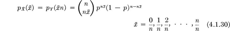
representing the number of successes (observations of “1’s”) in n Bernoulli trials, is binomial, B(n,p) [Sec. 3.1.2, Eq. (3.1.4a)]. Hence the distribution of ![]() = Y/n is [Sec. 2.3.1]
= Y/n is [Sec. 2.3.1]
which is a binomial-like distribution defined on noninteger values.
Illustration: Quality indicator In the process of setting up proposed statistical methods of quality control in highway construction, engineers have investigated data from old tests of a typical material quality indicator, such as the density of the subbase. The data were selected only from those sections of roads which had subsequently proved with use to show good performance. The purpose of this effort is to determine the reliability of the material tests as indicators of final road performances. It is desired to estimate what proportion p of these tests indicated poor material and consequently incorrectly suggested that the road would be of unsatisfactory quality. If X is a (0,1) Bernoulli random variable, indicating by a value “1” that the test would have rejected the (satisfactory) road, then in a sample of four sections of a road, the estimator ![]() of mX and hence of p has the distribution
of mX and hence of p has the distribution

Clearly the estimate of p is restricted to one of these five values, since only an integer number, 0, 1, 2, 3, or 4, of tests can be observed to be “bad.” The mean and variance of the estimator are
![]()
For example, if the true value of p were 10 percent, then![]() , the estimator of p, would have this distribution:
, the estimator of p, would have this distribution:
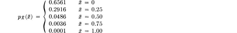
Thus, for example, if the engineers look at only four observations of a test of this kind, i.e., one which is actually incorrect only 10 percent of the time, there is a 5 percent chance that they will estimate that the test “rejects” potentially good roads half the time. If many independent samples of size four were taken (say, four sections from many different roads) and p estimated from each sample, the average (mean) of the estimate would be
![]()
and the square root of the mean square error (rms) of these many estimates would be

Normally distributed sample mean ![]() From Chap. 3 we know that the distribution of the sample means in the two illustrations in Sec. 4.1.1 are, respectively, normal,
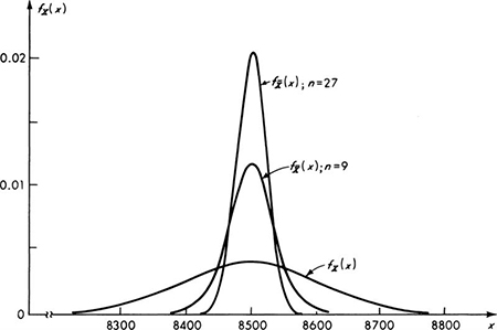
From Chap. 3 we know that the distribution of the sample means in the two illustrations in Sec. 4.1.1 are, respectively, normal, ![]() , and gamma, † G(n,nλ), for the normally distributed bar-yield-force variable and the exponentially distributed traffic-interval variable. Assuming that the true distribution of the bar-force data is normal, with mean 8500 lb and standard deviation 100 lb, this distribution and those of the sample means for two sample sizes, n = 9 and n = 27, are shown in Fig. 4.1.3. The distribution of
, and gamma, † G(n,nλ), for the normally distributed bar-yield-force variable and the exponentially distributed traffic-interval variable. Assuming that the true distribution of the bar-force data is normal, with mean 8500 lb and standard deviation 100 lb, this distribution and those of the sample means for two sample sizes, n = 9 and n = 27, are shown in Fig. 4.1.3. The distribution of ![]() , the mean of the exponentially distributed traffic intervals is skewed right for small sample sizes. As n increases, this gamma distribution will be almost perfectly symmetrical. In a few such cases the distribution of the sample mean is one of the common distributions discussed in Chap. 3. But in general when dealing with the distribution of the sample mean we rely upon another observation.
, the mean of the exponentially distributed traffic intervals is skewed right for small sample sizes. As n increases, this gamma distribution will be almost perfectly symmetrical. In a few such cases the distribution of the sample mean is one of the common distributions discussed in Chap. 3. But in general when dealing with the distribution of the sample mean we rely upon another observation.
Fig. 4.1.3 Bar-yield-force illustration—distributions of X and of two sample means ![]() ; n = 9, n = 27.
; n = 9, n = 27.
If n is reasonably large, we can invoke the central limit theorem (Sec. 3.3.1) to state that, no matter what the distribution of X, the sample mean will be approximately normal. Its mean is mx and its standard deviation is![]() . As the most important single case, we choose the normally distributed sample mean to illustrate the use to which the distribution of the sample statistic is put in estimation situations, namely, in the determination of interval estimates.
. As the most important single case, we choose the normally distributed sample mean to illustrate the use to which the distribution of the sample statistic is put in estimation situations, namely, in the determination of interval estimates.
Confidence intervals Consider again the problem of the yield force in reinforcing bars. Let us assume that through a history of tests on similar material and other bar sizes the engineer knows with relative certainty that the standard deviation of the yield force is 100lb. † His problem is to estimate the mean, and he focuses attention quite logically upon the sample mean![]() . This statistic is, prior to making the sample, a random variable normally distributed ‡ with unknown mean m and known standard deviation 100
. This statistic is, prior to making the sample, a random variable normally distributed ‡ with unknown mean m and known standard deviation 100 ![]() . Thus the variable
. Thus the variable ![]() /
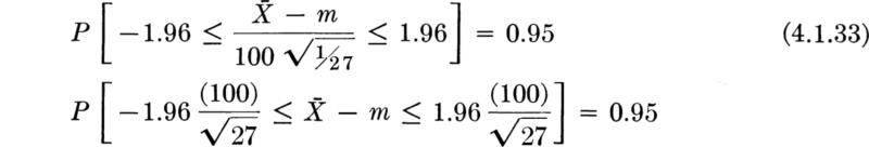
/![]() is N(0,l). Anticipating an experiment involving 27 specimens, the engineer can say, for example,
is N(0,l). Anticipating an experiment involving 27 specimens, the engineer can say, for example,
or
The statement, before experimentation, is that the sample average will with probability 0.95 lie within 37.7 lb of the true mean.
But what can be said after the experiment when the results in Table 4.1.1 are observed and ![]() is found to take on the value
is found to take on the value ![]() = 8490 lb? It is tempting to substitute
= 8490 lb? It is tempting to substitute ![]() for
for ![]() in the formula above, yielding
in the formula above, yielding
As inviting as it is to use the statement “the probability that the true mean lies in the interval 8452.3 and 8527.7 is 0.95” as a concise way of incorporating our uncertainty about the true value of the mean, the statement is, strictly speaking, inadmissible. The true mean of X has been considered, to this point, † to be a constant, not a random variable. As such, mx has a specific (although unknown) value, and it is not free to vary from experiment to experiment. It either lies in the stated interval or it does not.
Although the probability statement is not strictly correct in the present context, intervals formed in the manner above do convey a measure of the uncertainty associated with incomplete knowledge of parameter values. Such intervals are termed confidence intervals or interval estimates. The number which is the measure of this uncertainty is called the confidence coefficient. In this case the “95 percent confidence interval” that was observed in this particular experiment is 8452.3 to 8527.7.
The confidence interval provides an interval estimate on a parameter as opposed to the point estimates we considered earlier in the chapter. When the distribution whose parameter is being estimated is to be embedded in a still larger probabilistic model, the engineer can seldom afford the luxury of carrying along anything more than a point estimate, i.e., a single number, to represent the parameter. But the statement of an interval estimate does serve to emphasize that the value of a parameter is not known precisely and to quantify the magnitude of that uncertainty.
Confidence intervals on the mean Consider a more general statement concerning the confidence interval of the mean when σ is known. The statistic ![]() is assumed to be approximately (if not exactly) distributed, N(0,l). Hence
is assumed to be approximately (if not exactly) distributed, N(0,l). Hence
U being the standardized normal random variable. The limits a and b are usually chosen symmetrically, † and we write
in which k α/2 is denned to be that value such that 1 – FU(k α/2) = α/2. It is found in tables of the standardized normal distribution. Then
or
which is of the form
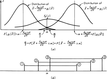
In this form it is clear that the two limits of the interval, g1![]() and g2
and g2![]() ,are sample statistics and random variables. ‡ Equation (4.1.40) states that the probability that these two random variables will bracket the true mean is 1 – α. The probability that either the lesser random variable g1
,are sample statistics and random variables. ‡ Equation (4.1.40) states that the probability that these two random variables will bracket the true mean is 1 – α. The probability that either the lesser random variable g1![]() will exceed m or the greater, g2
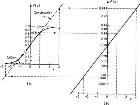
will exceed m or the greater, g2![]() , will be less than m is α. Figure 4.1.4 demonstrates these points.
, will be less than m is α. Figure 4.1.4 demonstrates these points.
The confidence interval on m with confidence coefficient (1 – α) 100 percent is formed after the experiment by substituting the observed value ![]() for
for ![]() . Thus the (1 – α) 100 percent confidence interval on m is
. Thus the (1 – α) 100 percent confidence interval on m is ![]() or
or ![]()
Fig. 4.1.4 (a) Distributions of confidence-limit statistics, g1![]() and g2
and g2![]() ; (b) three possible observed values of confidence limits g1
; (b) three possible observed values of confidence limits g1![]() ) to g2
) to g2![]() (two contain m, the third does not).
(two contain m, the third does not).
Factors influencing confidence intervals The engineer would prefer to report very tight intervals, that is, well-defined estimates of m. But notice that the width of the interval between these limits depends on three factors: σ, α, and n. The larger the standard deviation of X, the wider these intervals will be, and the intervals will be narrower if 1 – α is permitted to be smaller. The value of 1 – α can be interpreted as the long-run proportion of many (1 – α) 100 percent confidence intervals which will include the true mean. In the long run α 100 percent will fail to bracket the true mean. The choice of the value of α is the engineer’s, and depends in principle upon the importance associated with making the mistake of stating that an observed interval contains m when in fact it does not. In practice, the 90, 95, or 99 percent confidence intervals are reported. Decreasing α requires increasing the interval width, i.e., making a less precise statement about the value of m.
It is most important to observe that these confidence limits depend upon the sample size n. For a fixed confidence level, 1 – α, the interval can be made as short as the engineer pleases at the expense of additional sampling. If, on the other hand, the sample size has been fixed (and α is prescribed), the engineer must be content with the interval width associated with this amount of information. Precise statements with high confidence come only at the price of a sufficiently large sample.
Confidence intervals: typical procedure Confidence limits on a parameter are obtained, in general, in the following way:
1. Writing a probability statement about an appropriate sample statistic
2. Rearranging the statement to isolate the parameter
3. Substituting in the inequality the observed value of the sample statistic
Illustrations will make this procedure clear and bring out some additional points.
Illustration: The exponential case: one-sided intervals and confidence intervals on functions Recall the exponential illustration in Sec. 4.1.1. There the sample size was large, so we may assume that the estimator ![]() of the mean 1/λ is approximately normally distributed with mean
of the mean 1/λ is approximately normally distributed with mean ![]() and variance
and variance ![]() . The large sample size implies that the coefficient of variation of
. The large sample size implies that the coefficient of variation of ![]() , is small and that consequently the method-of-moments estimator of λ,
, is small and that consequently the method-of-moments estimator of λ, ![]() , is also approximately normally distributed † with approximate mean
, is also approximately normally distributed † with approximate mean ![]() and variance
and variance![]() . The implication is that the sample statistic
. The implication is that the sample statistic ![]() is approximately N(0,l).
is approximately N(0,l).
In the traffic-interval study suppose that interest lies in the possibility of the average arrival rate λ being so great that the gaps between cars are not long enough on the average to permit proper merging of traffic from a side road. The engineer would like a “conservative” lower bound estimate on the value of λ.
A one-sided probability statement on the sample statistic is called for. It should be
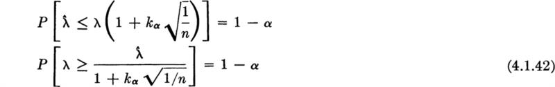
in which kα is that value of an N(0,l) variable which will be exceeded with probability α. Isolating the parameter of interest within the statement,
The random variable in this statement is, recall, ![]() . After the sample is taken, a one-sided (1 – α) 100 percent confidence interval on the parameter λ is found by substituting for the observed value of the random variable
. After the sample is taken, a one-sided (1 – α) 100 percent confidence interval on the parameter λ is found by substituting for the observed value of the random variable![]() . In this example, suppose a 95 percent level of confidence is desired; then α = 5 percent and k0.05 = 1.64 (Table A.l). A sample (Table 4.1.2) of size n = 214 yielded an observed value of
. In this example, suppose a 95 percent level of confidence is desired; then α = 5 percent and k0.05 = 1.64 (Table A.l). A sample (Table 4.1.2) of size n = 214 yielded an observed value of ![]() = 0.130 sec-1. Thus “with 95 percent confidence” λ is greater than
= 0.130 sec-1. Thus “with 95 percent confidence” λ is greater than

in words, 0.166 is a lower one-sided 95 percent confidence limit on λ.
Exact Distribution It is worth outlining how such a confidence interval would be obtained if the sample size were not sufficiently large to justify the assumption of normality. In principle the exact distribution of ![]() is needed, when, as pointed out above,
is needed, when, as pointed out above, ![]() has a gamma distribution. In this case, however, we can use the distribution of
has a gamma distribution. In this case, however, we can use the distribution of ![]() directly, since
directly, since
For given α and n, tables (Sec. 3.2.3) of the gamma distribution will give 1 / α as a function of the parameter λ. A rearrangement will isolate λ in the probability statement permitting the substitution of the observed value of ![]() and yielding an exact confidence interval on λ.
and yielding an exact confidence interval on λ.
Confidence Interval on a Function of a Parameter Engineering interest in estimated quantities usually goes beyond the values of the parameters themselves. If the model is incorporated into the framework of a larger problem, confidence intervals on functions of the parameters may be required. Consider the following elementary example. In the traffic situation above, the engineer might be interested in an estimate of the proportion of gaps which are larger than t0, the value required to permit another car to enter from a side road.† This proportion is
which is a function of the unknown parameter λ.
A point estimate of ![]() is simplyng
is simplyng![]() . If an upper, one-sided confidence interval on
. If an upper, one-sided confidence interval on ![]() is desired, the starting point is again an appropriate, rearranged probability statement on the sample statistic [Eq. (4.1.42)]:
is desired, the starting point is again an appropriate, rearranged probability statement on the sample statistic [Eq. (4.1.42)]:

Manipulating the inequality to isolate, not λ, but the function of λ of interest, namely, ![]() we obtain
we obtain

In words, a (1 – α) 100 percent upper confidence interval on the proportion of gaps greater than t0 is exp ![]() with the observed value of
with the observed value of ![]() substituted.
substituted.
In the numerical example above, with t0 = 10 sec, the 95 percent upper confidence interval on the proportion is

In words, the engineer would report that “with 95 percent confidence the proportion of gaps greater than 10 sec is less than 0.313.”
Notice that in this case the result coincides with the value obtained by substituting the lower bound of the 95 percent confidence interval on λ into the function of λ, ![]() . When a monotonic function is involved, such a simple substitution is always possible provided that thought is given to the type of bound on the parameter, upper or lower, which corresponds to the desired bound on the function. More difficult operations, analogous to those used in Sec. 2.3, are needed when confidence intervals on nonmontonic functions are encountered.
. When a monotonic function is involved, such a simple substitution is always possible provided that thought is given to the type of bound on the parameter, upper or lower, which corresponds to the desired bound on the function. More difficult operations, analogous to those used in Sec. 2.3, are needed when confidence intervals on nonmontonic functions are encountered.
Illustration: Variance of the normal case Confidence intervals on the variance of a random variable can be formed once the distribution of S2 is known. We consider here a special case—that in which the underlying variable X is normally distributed.
The determination of the distribution of S2 follows from available results. Consider the statistic S2 in Eq. (4.1.15). Adding and subtracting m and expanding the square gives
Multiplying by n/σ2, we find
The first term on the right-hand side is the sum of the squares of n independent normally distributed random variables each with zero mean and standard deviation 1. According to the results in Sec. 3.4.2, this sum has the χ2 distribution with n degrees of freedom. But the second term is also the square of a N (0,l) random variable since ![]() has been shown to be
has been shown to be![]() . Hence the second term has a χ2 distribution with 1 degree of freedom. Rewriting Eq. (4.1.47), we obtain
. Hence the second term has a χ2 distribution with 1 degree of freedom. Rewriting Eq. (4.1.47), we obtain
Equation (4.1.48) states that a ![]() random variable is the sum of nS2/σ2 and a
random variable is the sum of nS2/σ2 and a ![]() random variable. Knowing, as shown in Sec. 3.4.2, that the sum of two independent χ2 random variables, one with r degrees of freedom and the other with p, is χ2-distributed with r + p degrees of freedom, it is not unexpected (what is shown here is not a proof†) that nS2/ σ2 is χ2-distributed with n – 1 degrees of freedom. The same is true of (n – 1)S2* /σ2.
random variable. Knowing, as shown in Sec. 3.4.2, that the sum of two independent χ2 random variables, one with r degrees of freedom and the other with p, is χ2-distributed with r + p degrees of freedom, it is not unexpected (what is shown here is not a proof†) that nS2/ σ2 is χ2-distributed with n – 1 degrees of freedom. The same is true of (n – 1)S2* /σ2.
With this knowledge confidence intervals follow easily. For example, begin with the probability statement
in which ![]() that (tabulated) value ‡ such that, if Y is CH(n – 1), then
that (tabulated) value ‡ such that, if Y is CH(n – 1), then ![]() We are led to a (1 – α) 100 percent one-sided confidence interval on σ2 by rearrangement:
We are led to a (1 – α) 100 percent one-sided confidence interval on σ2 by rearrangement:
For example, in the bar-yield-force illustration, the 99 percent upper confidence limit on σ2 is (Table A.2)
![]()
Owing to the monotonic relationship between the variance and standard deviation, the square roots of variance confidence interval bounds are the bounds of the corresponding confidence limits on the standard deviation. In this example a 99 percent one-sided upper confidence interval on σ is ![]() or
or ![]() = 158 lb.
= 158 lb.
Illustration: Mean of the normal case, variance unknown; experimental design Interval estimates on the mean are usually based on the assumption that the sample statistic ![]() is normally distributed with mean m and variance σ2/n. This case has been considered in detail above under the assumption that σ2 was known. If, as is more common, the variance is not known, other approaches are necessary. In some cases the unknown variance may be simply related to the unknown mean. This is the case if the distribution of X has only a single unknown parameter. (Examples are: the exponential distribution, the binomial distribution, or the normal distribution with known coefficient of variation.) In this case relatively simple intervals are possible, as before. See, for example, the first paragraph of the preceding illustration of the exponential parameter. In other cases, if the sample size is sufficiently large, it is reasonable (see Brunk [I960]) to set up the confidence interval assuming that σ2 is known and then simply replace σ2 by its estimate S2 after the test results are obtained. In other words, the statistic
is normally distributed with mean m and variance σ2/n. This case has been considered in detail above under the assumption that σ2 was known. If, as is more common, the variance is not known, other approaches are necessary. In some cases the unknown variance may be simply related to the unknown mean. This is the case if the distribution of X has only a single unknown parameter. (Examples are: the exponential distribution, the binomial distribution, or the normal distribution with known coefficient of variation.) In this case relatively simple intervals are possible, as before. See, for example, the first paragraph of the preceding illustration of the exponential parameter. In other cases, if the sample size is sufficiently large, it is reasonable (see Brunk [I960]) to set up the confidence interval assuming that σ2 is known and then simply replace σ2 by its estimate S2 after the test results are obtained. In other words, the statistic ![]() used in Eq. (4.1.36) is replaced by the statistic
used in Eq. (4.1.36) is replaced by the statistic![]() , but the uncertainty associated with not knowing σ2 is ignored.
, but the uncertainty associated with not knowing σ2 is ignored.
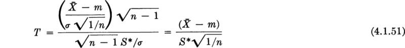
In smaller samples this contribution cannot be ignored, however, and, if one of the latter statistics is to be used, its true distribution must be found. This has been done for the case when X is normal. Multiplying numerator and denominator by![]() , the second statistic † above, i.e., the so-called t statistic, takes on a recognizable form:
, the second statistic † above, i.e., the so-called t statistic, takes on a recognizable form:
The numerator is ![]() times a N(0,l) random variable. The denominator being the square root of the χ2-distributed variable, (n – 1)S2*/σ2, is χ-distributed, CHI(n – 1), as defined in Sec. 3.4.3. In that same section a variable of the form of T was said to have the “t distribution” with n – 1 degrees of freedom, if numerator and denominator are independent. That S2* and
times a N(0,l) random variable. The denominator being the square root of the χ2-distributed variable, (n – 1)S2*/σ2, is χ-distributed, CHI(n – 1), as defined in Sec. 3.4.3. In that same section a variable of the form of T was said to have the “t distribution” with n – 1 degrees of freedom, if numerator and denominator are independent. That S2* and ![]() , both functions of the same n normally distributed random variables X1, X2, . . ., Xn, are independent is hardly to be expected, but is in fact true. The verification is lengthy and will not be shown here.‡
, both functions of the same n normally distributed random variables X1, X2, . . ., Xn, are independent is hardly to be expected, but is in fact true. The verification is lengthy and will not be shown here.‡
The t statistic, Eq. (4.1.51), has a somewhat broader distribution than the corresponding normally distributed statistic, ![]() , associated with a known standard deviation σ. See Fig. 3.4.4. This fact merely reflects the greater uncertainty which is introduced if there is a lack of knowledge of the true value of σ. For the same value of 1 – α, we should expect somewhat wider confidence intervals on m in this case. This will be demonstrated.
, associated with a known standard deviation σ. See Fig. 3.4.4. This fact merely reflects the greater uncertainty which is introduced if there is a lack of knowledge of the true value of σ. For the same value of 1 – α, we should expect somewhat wider confidence intervals on m in this case. This will be demonstrated.
Having at hand the distribution of the statistic ![]() (see Table A.3), we can find a confidence interval on m by following the usual pattern.
(see Table A.3), we can find a confidence interval on m by following the usual pattern.
Write an appropriate probability statement:
in which tα/2,n–1 is that (tabulated) value which a random variable with a t distribution with parameter n – 1 exceeds with probability α/2.
Isolate the parameter of interest:
Substitute in the inequality the observed values of the sample statistics. The (1 – α) 100 percent two-sided confidence interval on m is
In the bar-yield force example with n = 27, ![]() = 8490, and s* = 105, the 95 percent confidence intervals on m are
= 8490, and s* = 105, the 95 percent confidence intervals on m are

which, upon substitution from Table A.3 of t0.025,26 = 2.056, yields
![]()
These limits are wider by a factor 2.056/1.963 = 1.05 than those which would be obtained if σ had been assumed to be known with certainty to equal the observed yalue of S*, namely, 105 lb. For sample sizes of 5, 10, and 15 this factor is 1.31, 1.16, and 1.08. For sample sizes larger than about 25, it is clearly usually sufficient to use the test based on the normal distribution assuming σ = s*. In other words, for large n, T is very nearly N(0,l) (see Fig. 3.4.4).
Choice of Sample Size The engineer is occasionally in a situation where he can “design” his sampling procedure to yield confidence limits of a desired width with a prescribed confidence. In other words he can determine n, the sample size needed to yield an estimate of m, say, with specified accuracy and confidence.
Consider the following example. It is typical of practice recommended by the American Concrete Institute for determining the required number of times to sample a batch of concrete in order to estimate its mean strength for quality control purposes. The strength is assumed to be normally distributed. Assume that we desire a one-sided, lower, 90 percent confidence interval on the mean which has an interval width of no more than about 10 percent of the mean. Considering a one-sided version of Eq. (4.1.54), we want to pick n such that

It has been observed that the coefficient of variation of concrete strength under fixed conditions of control remains about constant when the mean is altered. (See Prob. 2.45.) Here, say it is about 15 percent. Thus we expect s* to be about 0.15![]() , and we seek n such that
, and we seek n such that

Using Table A.3, we find that a value of n equal to 5 gives

A sample of size five should be used to meet the stated specifications.
After taking a sample of size 5 and observing, for example, ![]() = 4000 psi and s* = 700 psi, the engineer could say, with 90 percent confidence, that the true mean is greater than
= 4000 psi and s* = 700 psi, the engineer could say, with 90 percent confidence, that the true mean is greater than

Notice that the required number of samples depends upon the desired confidence, the desired width of the interval, and the estimated coefficient of variation of the concrete strength (the last is considered a measure of the quality of the control practiced by the contractor).
Comments For the reasons stated in this section the engineer who has, for example, observed ![]() and calculated confidence limits should not say “The probability that m lies between
and calculated confidence limits should not say “The probability that m lies between![]() ,” but rather just “the (1 – α) 100 percent confidence limits on m are
,” but rather just “the (1 – α) 100 percent confidence limits on m are ![]()
![]() ” Superficially, the distinction may seem to be one of semantics only, but it is of fundamental importance in the theory of statistics. The reader will, however, hear statements like the former one made by engineers who use statistical methods frequently. Such “probability statements” remain the most natural way of describing the situation and of conveying the second kind of uncertainty, that surrounding the value of a parameter. Consequently, such statements should probably not be discouraged, as they seem to express the way engineers operate with such limits. Fortunately, the more liberal interpretation of probability, namely, that associated with degree of belief (Sec. 2.1 and Chap. 5) permits and encourages this pragmatic, operational use of confidence limits, as we shall see in Chap. 6.
” Superficially, the distinction may seem to be one of semantics only, but it is of fundamental importance in the theory of statistics. The reader will, however, hear statements like the former one made by engineers who use statistical methods frequently. Such “probability statements” remain the most natural way of describing the situation and of conveying the second kind of uncertainty, that surrounding the value of a parameter. Consequently, such statements should probably not be discouraged, as they seem to express the way engineers operate with such limits. Fortunately, the more liberal interpretation of probability, namely, that associated with degree of belief (Sec. 2.1 and Chap. 5) permits and encourages this pragmatic, operational use of confidence limits, as we shall see in Chap. 6.
The use of confidence limits is most appropriate in reporting of data. It provides a convenient and concise method of reporting which is understood by a wide audience of readers, and which encourages communication of measures of uncertainty as well as simply “best” (or point) estimates of parameters. In spite of the somewhat arbitrary nature of the conventionally used confidence levels, and in spite of the philosophical difficulties surrounding their interpretation, confidence limits remain, therefore, useful conventions.
A widely used rule for choosing the sample† statistic to be used in estimation often replaces the method of moments described in Sec. 4.1.1. This is called the method of maximum likelihood. In addition to prescribing the statistic which should be used, it provides an approximation of the distribution of that statistic, so that approximate confidence intervals may be constructed.
The likelihood function The method of maximum likelihood makes use of the sample-likelihood function. Suppose for the moment that we know the parameter(s) θ of the distribution of X. Then we can write down the joint probability distribution of a (random) sample X1, X2, . . ., Xn,

The expression has been written in a manner, f(· | θ), which emphasizes that the parameter is known. If, for example, the underlying random variable is T and it has an exponential distribution with parameter λ,
Placing ourselves now in a position of having sampled and observed specific values X1 = x1, X2 = x2, . . ., Xn = xn, but not knowing the parameter θ, we can look upon the right-hand side of the function above [Eq. (4.1.54)] as a function of θ only. It gives the relative likelihood of having observed this particular sample, x1, x2, . . ., xn, as a function of θ. To emphasize this, it is written
and is called the likelihood function of the sample. For the exponential example, the observed values t1, t2, .. ., tn determine a number ![]() , and the likelihood function of the parameter λ is
, and the likelihood function of the parameter λ is
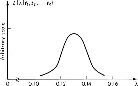
The likelihood function is sketched in Fig. 4.1.5 for the data reported in Table 4.1.2. The vertical scale is arbitrary, since only relative values will be of interest.
The likelihood function is subject also to a looser, inverse interpretation. It can be said to give, in addition to the relative likelihood of the particular sample for a given θ, the relative likelihood of each possible value of θ given the sample. This intuitively appealing interpretation suggests that values of θ for which the observed sample was relatively speaking more likely, are, relatively speaking, the more likely values of the unknown parameter θ. In Fig. 4.1.5, for example, values of λ between 0.12 and 0.14 are, in light of the observed sample, “more likely” to be the true value of λ than a value near 0.10 or 0.16. Likelihood functions will be used extensively in Chaps. 5 and 6 to represent the information contained in the observed sample about the relative likelihoods of the various possible parameter values.
Fig. 4.1.5 Traffic-interval illustration: likelihood function on λ.
Maximum-likelihood criterion for estimation The likelihood function is used to determine parameter estimators. Formally, the rule for obtaining a maximum-likelihood estimator is:
The maximum-likelihood estimator of θ is the value ![]() which causes the likelihood function L(θ) to be a maximum.
which causes the likelihood function L(θ) to be a maximum.
For example, in the exponentially distributed traffic-interval illustration, it is clear from Fig. 4.1.5 that the most likely value of λ, i.e., the maximum-likelihood estimate of λ, is about 0.13. More generally we seek ![]() to maximize Eq. (4.1.57):
to maximize Eq. (4.1.57):
Any of the many techniques for seeking the maximum of a function are acceptable. One which is frequently appropriate in maximum-likelihood estimation problems is to find the maximum of the logarithm of the function† by setting its derivative equal to zero. Here:
The derivative (with respect to λ), when set equal to zero, yields
Solving for ![]() , the value which maximizes In L (and L),
, the value which maximizes In L (and L),
which equals ![]() and hence (only coincidentally) is equivalent to the estimator suggested by the method of moments, Eq. (4.1.7).
and hence (only coincidentally) is equivalent to the estimator suggested by the method of moments, Eq. (4.1.7).
The two estimators, given by the method of moments and the method of maximum likelihood, may not be identical. The reader is asked to show in Prob. 4.20 that the method-of-moments estimator of the parameter b of a random variable known to have distribution uniform on the interval 0 to b is 2![]() , and the maximum-likelihood estimator is X(n) =
, and the maximum-likelihood estimator is X(n) = ![]() , the largest observed value in the sample. Note that the method of moments might lead to an estimated value of the theoretical upper value b that is less than the largest value observed!
, the largest observed value in the sample. Note that the method of moments might lead to an estimated value of the theoretical upper value b that is less than the largest value observed!
Two or more parameters It should be clear that these notions can be easily generalized to those situations where two or more (say r) parameters must be estimated to define a distribution. Call this vector of parameters θ = {θ1, θ2, . . . , θr}. The method of maximum likelihood states: choose the estimators ![]() to maximize the likelihood
to maximize the likelihood
or, equivalently, the log likelihood (if appropriate to the particular problem)
This maximization will typically require solving a set of r equations
The solution may also be subject to certain constraints, for example, ![]() > 0 or
> 0 or ![]() max [xi]. The solution of the system is not always possible in closed form; in complex problems, computer-automated trial-and-error search techniques are often employed to find the
max [xi]. The solution of the system is not always possible in closed form; in complex problems, computer-automated trial-and-error search techniques are often employed to find the ![]() values which maximize the likelihood function.
values which maximize the likelihood function.
Illustration: Maximum-likelihood estimators in the normal case As an illustration, we seek the maximum-likelihood estimators of the parameters m and σ of the normal distribution when both are unknown. The likelihood function is
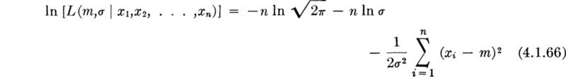
The presence of exponentials suggests in this case an attack on the log-likelihood function
To choose ![]() and
and ![]() to maximize this function, we set the partial derivatives equal to zero:
to maximize this function, we set the partial derivatives equal to zero:
and solve these simultaneous equations for ![]() and
and ![]() . Since 0 < σ < ∞, the former equation is satisfied only if
. Since 0 < σ < ∞, the former equation is satisfied only if
Substituting this expression into the second equation and solving for ![]() gives
gives
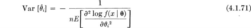
Properties of maximum-likelihood estimators As sample statistics or functions of the observations, the estimators are, before the experiment, random variables and can be studied as such. In fact, the major advantage of maximum-likelihood estimators is that their properties have been thoroughly studied and are well known, virtually independently of the particular density function under consideration. Noting the summation form of Eq. (4.1.64), one should not be surprised to learn that the estimators ![]() are approximately (for large n), normally distributed.† Their means are (asymptotically, as n → ∞) equal to the true parameter values θ ; that is, the estimators are asymptotically unbiased. Their variances (or mean square errors) are (asymptotically) equal to
are approximately (for large n), normally distributed.† Their means are (asymptotically, as n → ∞) equal to the true parameter values θ ; that is, the estimators are asymptotically unbiased. Their variances (or mean square errors) are (asymptotically) equal to
For example, the approximate variance of the estimator of the parameter λ in the exponential illustration is found as follows:
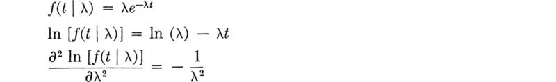
In this case the result is simply a constant independent of the random variable T. Therefore, the expectation is simply that of a constant or the constant itself:

and [Eq. (4.1.71)]

An estimate of this approximate variance is found by substituting ![]() for λ, which gives
for λ, which gives ![]() .
.
In the car-following data the standard deviation of ![]() , the estimator of λ, is approximately
, the estimator of λ, is approximately

Note once again the characteristic decrease in the expected square error of an estimator by a factor 1/n.
In addition to being asymptotically unbiased (that is, ![]() ), the maximum-likelihood estimators can be shown (e.g., Freeman [1963]) to have, at least asymptotically, the additional desirable properties that they have minimum expected squared error among all possible unbiased estimators (hence they are said to be efficient). They also generally give the same estimator for a function of a parameter g(θ) as that found by simply substituting the estimator† of θ, that is,
), the maximum-likelihood estimators can be shown (e.g., Freeman [1963]) to have, at least asymptotically, the additional desirable properties that they have minimum expected squared error among all possible unbiased estimators (hence they are said to be efficient). They also generally give the same estimator for a function of a parameter g(θ) as that found by simply substituting the estimator† of θ, that is, ![]() =
= ![]() (i.e., they are said to be invariant); they will with increasingly high probability be arbitrarily close to the true values (i.e., they are said to be consistent)) and they make maximum use of the information contained in the data (i.e., they are said to be sufficient). If the available sample sizes are large, there seems little doubt that the maximum-likelihood estimator is a good choice. It should be emphasized, however, that the properties above are asymptotic (large n), and better (in some sense) estimators† may be available when sample sizes are small.
(i.e., they are said to be invariant); they will with increasingly high probability be arbitrarily close to the true values (i.e., they are said to be consistent)) and they make maximum use of the information contained in the data (i.e., they are said to be sufficient). If the available sample sizes are large, there seems little doubt that the maximum-likelihood estimator is a good choice. It should be emphasized, however, that the properties above are asymptotic (large n), and better (in some sense) estimators† may be available when sample sizes are small.
In this section we have investigated the problem of obtaining from data estimates of the parameters of a probabilistic model, such as a random variable X. We worked with estimators (i.e., certain functions of the sample, X1, X2, . . ., Xn); the estimators considered were those suggested by general rules, either the method of moments (Sec. 4.1.1) or the method of maximum likelihood (Sec. 4.1.4).
The customary estimator of the population mean mX is the sample mean ![]() :
:

while the conventional estimate of the variance σx2 is the sample variance, defined either as

or as

The choice between these estimators is not clear-cut, but the latter is used somewhat more frequently in practice.
An estimator ![]() is studied by familiar methods once it is recognized that it is a random variable and a function of X1 X2 . . ., Xn. The estimator’s mean E
is studied by familiar methods once it is recognized that it is a random variable and a function of X1 X2 . . ., Xn. The estimator’s mean E ![]() is compared with the true value of the parameter d. If they are equal, the estimator is said to be unbiased. The mean square error of any estimator is the sum of its variance and its squared bias, E
is compared with the true value of the parameter d. If they are equal, the estimator is said to be unbiased. The mean square error of any estimator is the sum of its variance and its squared bias, E![]() – θ is,
– θ is,
![]()
Generally we seek unbiased estimators with small mean square errors.
The distribution of an estimator can be used to obtain confidence-interval estimates on a parameter at prescribed confidence levels. These are obtained by “turning inside out” probability statements on the estimator ![]() to obtain random limits
to obtain random limits ![]() and
and ![]() which are (1 – α) 100 percent likely to contain the true parameter. After a sample has been observed, these limits are evaluated and called the (1 – α) 100 percent confidence interval on the true parameter.
which are (1 – α) 100 percent likely to contain the true parameter. After a sample has been observed, these limits are evaluated and called the (1 – α) 100 percent confidence interval on the true parameter.
A very common and most vexing problem that engineers face is the assessment of significance in scattered statistical data. For example, given a set of observed concrete cylinder strengths, say 4010, 3880, 3970, 3780, and 3820 psi, should a materials engineer report that the true mean strength of the batch of concrete is less than the design value of 4000 psi? Or to put the question differently, in light of the inherent variation in such observations, is the observed sample average
![]()
significantly less than the presumed value of 4000 psi? If the engineer had twice as many samples, but their average happened to be the same, 3892 psi, would this not be a “more significant” deviation from the presumed mean? Suppose an engineer has installed a new traffic-control device in an attempt to enhance the safety of an intersection. In the 3 months prior to the installation there were four major accidents there; in the 3 months following the installation there were two. Can the engineer conclude with confidence that the device has been effective? That is, has it reduced the mean accident rate? Is this limited data sufficient to justify such a conclusion? In different words, is the difference between 4 and 2 significant when one recognizes the inherently probabilistic nature of accident occurrences?
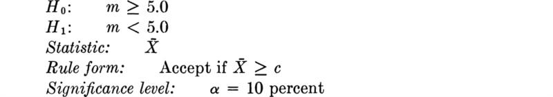
Generally speaking we state such problems as follows. The engineer considers a particular assumption about his model (e.g., “the true mean strength is 4000 psi” or “the mean accident rate is unchanged”). Given data, he wants to evaluate this tentative hypothesis. If the hypothesis is assumed to be correct, the engineer can calculate the expected results of an experiment. If the data are observed to be significantly different from the expected results, then the engineer must consider the assumption to be incorrect. The technical question to be answered is, “What represents a significant difference?”
Although many such problems in engineering are most effectively treated in the context of the modern decision theory to be presented in Chaps. 5 and 6, a simpler procedure has also been developed. Like confidence limits, this method of assessing the significance of data has the merit of being a widely used convention. Its use is therefore a convenient way to communicate to others the method by which the data were analyzed and the criterion by which the assumption or model was judged.
In this section we shall concentrate on relatively simple model assumptions; in particular, we shall test hypotheses about model parameter values. In Sec. 4.4 we shall treat the verification of the model or distribution as a whole, including its shape as well as its parameters.
This conventional procedure for drawing simple conclusions from observed statistical data is called hypothesis testing. Typical examples include: a product-development engineer who wants to decide whether or not a new concrete additive has a significant influence on curing time; a soils engineer who wants to report whether a simple, in-the-field “vane test” provides an unbiased estimate of the lab-measured unconfined compressive strength of soil; and a water-resources engineer who wants to verify an assumption used in his system model, namely, that the correlation coefficient between the monthly rainfalls on two particular watersheds is zero.
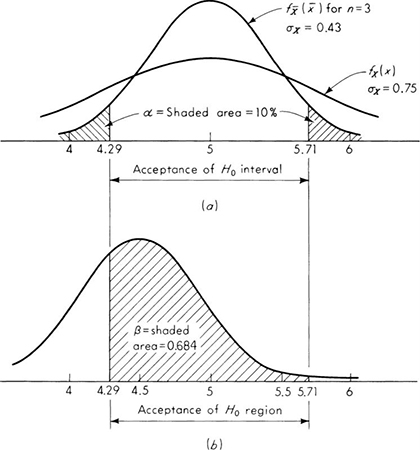
We shall develop the conventional treatment of such problems through the following simple example. Even under properly controlled production, asphalt content varies somewhat from batch to batch. A materials-testing engineer must report, on the basis of three batches, whether the mean asphalt content of all batches of material leaving a particular plant is equal to the desired value of 5 percent. The concern is that unknown changes in the mixing procedure or raw materials supply might have increased or decreased this mean. Based on previous experience the engineer is certain that, no matter what the mean, the asphalt content in different batches can be assumed to be normally distributed with a known standard deviation of 0.75 percent.
It is important to appreciate the basic dilemma. The engineer must use information in the sample to make his decision. This information is usually summarized in some sample statistic, such as the sample average ![]() . The finite size of the sample implies that any sample statistic calculated from the observations is a random variable with some nonzero variance. For example,
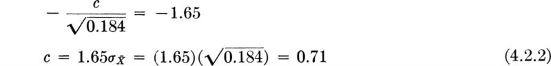
. The finite size of the sample implies that any sample statistic calculated from the observations is a random variable with some nonzero variance. For example, ![]() is a normally distributed random variable with a variance of (0.75) 2/3 = (0.43)2 = 0.184 and a mean m equal to the (unknown) true mean of the plant’s present production. Therefore the observed value of this sample statistic may lie some distance from the expected value of 5 even if this is the true value of the mean. On the other hand, if the true value of the mean asphalt content is no longer 5 but has slipped to 4.5 or increased to 5.6, the observed sample average may nonetheless lie close to the hypothesized value of 5. Thus, with limited data, the engineer cannot hope to be correct every time he makes a report. In some cases he will report that the mean is not 5 when it is; and in other cases he will report that it is 5 when it is not. At best he can ask for an operating rule which recognizes the inherent variability of the data and the size of his sample, and which promises some consistency in approach to this and similar questions he must report on. Preferably he would like to have some measure, too, of the percentage of times he will make one mistake or the other.
is a normally distributed random variable with a variance of (0.75) 2/3 = (0.43)2 = 0.184 and a mean m equal to the (unknown) true mean of the plant’s present production. Therefore the observed value of this sample statistic may lie some distance from the expected value of 5 even if this is the true value of the mean. On the other hand, if the true value of the mean asphalt content is no longer 5 but has slipped to 4.5 or increased to 5.6, the observed sample average may nonetheless lie close to the hypothesized value of 5. Thus, with limited data, the engineer cannot hope to be correct every time he makes a report. In some cases he will report that the mean is not 5 when it is; and in other cases he will report that it is 5 when it is not. At best he can ask for an operating rule which recognizes the inherent variability of the data and the size of his sample, and which promises some consistency in approach to this and similar questions he must report on. Preferably he would like to have some measure, too, of the percentage of times he will make one mistake or the other.
Hypothesis testing is a method which is commonly used in such routine decisions. It provides most of these desired consistency properties, and, being a widely used convention, it simplifies communication among engineers. If the materials engineer reports that he “accepted the hypothesis that the true mean is 5 at the 10 percent significance level/’ trained readers of the report will know first, and most importantly, that the engineer has studied and considered the scatter in the data, and, second, precisely the way by which he reached his conclusion, complete with the implied risks and limitations. The method is objective in that, under the convention, two engineers faced with the same data will report the same conclusion.
Application of the method In this example, the engineer using an hypothesis test would tentatively propose the null hypothesis H0 that the true mean is 5. He seeks a rule by which he can judge (i.e., accept or reject) this hypothesis on the basis of the observed asphalt content in the three specimens. A reasonable choice for this operating rule †is:
Accept the null hypothesis if the sample average ![]() lies within ± c of 5. Otherwise reject this hypothesis.
lies within ± c of 5. Otherwise reject this hypothesis.
Rejection of the null hypothesis implies (under this method) acceptance of the alternate hypothesis H1. In this case, the alternate hypothesis is simply that the mean is not 5 percent.
Once the form of this rule is chosen, the method of hypothesis testing provides a convention by which to determine the value of c. The method suggests:
Choose c such that there is only a prescribed (small) probability α, say 10 percent, that the sample mean of any three specimens will lie outside 5 ± c, given that the null hypothesis holds.
We know the probability distribution of ![]() given that the null hypothesis H0 holds. That distribution is N(5,0.184). Therefore, we can easily find c from the statement (Fig. 4.2.1a)
given that the null hypothesis H0 holds. That distribution is N(5,0.184). Therefore, we can easily find c from the statement (Fig. 4.2.1a)
In terms of the standardized normal distribution we want c such that

From tables,
Thus the operating rule becomes:
Accept the null hypothesis that the true mean is 5 if the observed value of the sample average lies between 5 ± 0.71 (that is, 4.29 and 5.71). Otherwise, reject the hypothesis.
Discussion The intuitive justification for this rule of operation is that if the observed sample mean is a “significant distance” from the assumed value, the assumption is probably wrong. Under the method, significant distance can be interpreted quantitatively as being a discrepancy c which would only be exceeded with a small probability if the hypothesis were true. If a discrepancy of that size or greater is observed, the method suggests that the engineer act as if his assumption were not true rather than accept the observation as a “rare event.” Although the conclusion will clearly depend upon the value of α chosen, the method does demand a rational analysis of uncertainty, namely, the study of the probabilistic behavior of the sample statistic used in the operating rule. If, for example, the standard deviation between individual batches (σx or 0.75) is different, or if the sample size is different, the value of c in the operating rule will also change.
Type I errors The values used for α, which is called the significance level of the test, are virtually always chosen by convention to be 10, 5, or 1 percent. In principle, but seldom in practice, one chooses α to reflect the consequences of making the mistake of rejecting the hypothesis when in fact it is true. If one always uses α = 5 percent, he will make this kind of mistake (the so-called type I error) 5 percent of the time in the long run. It is the authors’ experience and recommendation that the significance
Fig. 4.2.1 Type I and type II error probabilities for the asphalt-content operating rule, (a) Distribution of ![]() if m = 5, showing α, the probability of making type I error; (b) distribution of
if m = 5, showing α, the probability of making type I error; (b) distribution of ![]() if m = 4.5 showing the probability of type II error β.
if m = 4.5 showing the probability of type II error β.
level of a hypothesis test continue to be chosen simply by convention, say at the most commonly used 5 percent level. A thorough decision analysis requires explicit inclusion of costs or consequences and is best done using statistical decision theory (Chaps. 5 and 6).
Once the operating rule has been determined, the engineer need only obtain the data, calculate the statistic used in the rule, compare it with the acceptance interval, and accept or reject the hypothesis according to prescription. For example, if the materials engineer measured the asphalt content in three batches and found x1 = 4.2, x2 = 4.7, and x3 = 3.7, the observed sample mean would be ![]() = 4.2. Since this value lies outside the interval 4.29 to 5.71, he should reject the null hypothesis that the true mean is 5.0. In this case, the observed statistic would be said to be statistically significant at the 10 percent level, and the engineer would report that† he rejected the hypothesis that m = 5.0 at the 10 percent significance level.
= 4.2. Since this value lies outside the interval 4.29 to 5.71, he should reject the null hypothesis that the true mean is 5.0. In this case, the observed statistic would be said to be statistically significant at the 10 percent level, and the engineer would report that† he rejected the hypothesis that m = 5.0 at the 10 percent significance level.
Type II errors It must be recognized that one cannot afford to make the probability α of making a type I error arbitrarily small. This probability of rejecting H0 when it is true can only be made small at the expense of increasing the probability of a type II error, which is one of accepting H0 when it is not true.
Consider again the asphalt tests. The engineer might be concerned if either the true mean asphalt content were low, say 4.5 percent, or if it were high, say 5.5 percent. In either situation there is a possibility that the sample average will lie in the rule’s acceptance interval, 4.29 to 5.71. If this happens, the operating rule which the hypothesis-testing method has proposed will mistakenly suggest that the engineer act as if the true mean were 5. The probability of this possibility is called β. It can be evaluated for any particular value of the true mean. For example, if the true mean is 4.5, then for this operating rule (recall that α = 10 percent) the probability of incorrectly accepting the assumption that the mean m is 5 is
If the true mean is 4.5, the sample average is distributed N (4.5,0.184), implying (Fig. 4.2.1b)
Clearly, when the true mean is 4.5, the engineer using this method will, more often than not, mistakenly assume that the true mean is 5. If the true mean is 4, the type II error probability is reduced to about 25 percent, and if the true mean is 6.5, the β probability is only 3 percent. One can plot, as in Fig. 4.2.2, the error probability β as a function of the true mean m. Such a curve is called the operating characteristic (OC) curve of the rule. (Note that it equals 1 – α at m = 5.)
If the type II error probabilities implied by the operating rule are not tolerable, the engineer can, with some expense, reduce them. Either he may reduce the width of the acceptance interval ± c at the expense of increasing α, the type I error probability (see Fig. 4.2.1), or he may increase the sample size from three to some larger value. At the same
Fig. 4.2.2 The operating characteristic curve for the asphalt-content operating rule, α = 10 percent, with a sample size of three or six.
significance level, α = 10 percent, the increased sample size will reduce σ![]() and hence the interval width ± c [Eq. (4.2.2)]; at the same time it will change the shape of the distribution of
and hence the interval width ± c [Eq. (4.2.2)]; at the same time it will change the shape of the distribution of ![]() given that m = 4.5, say. The net effect will be a set of β values everywhere less than those for a sample size of three. For example, for a sample size of six, and α = 10 percent, c = 0.50 and the OC curve of β probabilities appears as indicated in Fig. 4.2.2.
given that m = 4.5, say. The net effect will be a set of β values everywhere less than those for a sample size of three. For example, for a sample size of six, and α = 10 percent, c = 0.50 and the OC curve of β probabilities appears as indicated in Fig. 4.2.2.
Choice of sample size If the engineer would like to obtain some prescribed level of “reliability” in his reporting method, he can calculate the sample size necessary to achieve it. For example, to keep α at 10 percent and also to reduce β to at most 20 percent when the true mean is 4.5, one can easily calculate that the sample size must be at least 14. If this amount of testing is unduly expensive, some tradeoff between sampling cost, type I error, and type II errors must be made. Such decisions are probably best made in a totally economic context such as that to be discussed in Chaps. 5 and 6. We will restrict attention in this chapter to analysis of data from a fixed sample size and under a conventional level of significance (say, α = 5 percent), accepting the implied levels of β.
In this section we will summarize the hypothesis-testing method and then present briefly a number of common hypothesis tests, using them to bring out some additional points about the method.
Procedure summary Generally speaking, the engineer has an assumption about his model and certain data. The object is to determine if the observations display characteristics significantly different from those expected under the assumption. The steps are:
1. Identify the null hypothesis H0 and the alternate hypothesis H1.
2. Select an appropriate sample statistic to be used in the test.
3. Select an appropriate form for the operating rule, usually up to a constant c. The rule must divide the sample space of the sample statistic into two mutually exclusive, exhaustive events, one to be associated with acceptance of H0, the other with rejection.
4. Select a significance level α at which to run the test.
5. Use the distribution of the sample statistic to determine the value of the constant c so that when H0 is true, there is a probability α of rejecting that hypothesis.
6. If appropriate and feasible, investigate the type II error probabilities associated with the chosen rule, assuming that H1 rather than H0 holds.
7. Carry out the test by calculating the observed value of the sample statistic and comparing it with the acceptance and rejection regions defined by the rule.
8. If the observed sample statistic falls in the rejection region (or critical region), announce that it is “significant at the α percent level” and reject the hypothesis. If the statistic falls in the acceptance region, accept H0.
We saw in the last section an extended example of a case which can be summarized as follows:
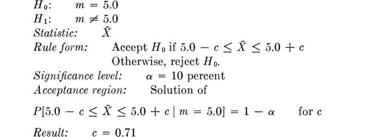
In this example, the variance of the underlying random variable X was assumed to be known to be (0.75)2; the sample size was three; ![]() was assumed to be normally distributed with variance (0.75)2/3. Notice that this would be the case no matter what the distribution of X as long as the engineer is prepared to assume that,
was assumed to be normally distributed with variance (0.75)2/3. Notice that this would be the case no matter what the distribution of X as long as the engineer is prepared to assume that, ![]() is normally distributed. In general, of course, the exact distribution of
is normally distributed. In general, of course, the exact distribution of ![]() should be used. As we have seen in Sec. 4.1, this will depend upon the distribution of X. For example, if
should be used. As we have seen in Sec. 4.1, this will depend upon the distribution of X. For example, if ![]() is Bernoulli,
is Bernoulli, ![]() is binomial (Sec. 4.1.3). In such discrete cases one cannot usually find a value of c (since nc must be integer) to exactly meet the desired significance level α.
is binomial (Sec. 4.1.3). In such discrete cases one cannot usually find a value of c (since nc must be integer) to exactly meet the desired significance level α.
One-sided versus two-sided tests; simple versus composite hypotheses Other forms of hypotheses might be more appropriate in the asphalt illustration. For example, the engineer may know that if the mean is not equal to m0 (say, 5) then it is surely equal to m1 (say, 4.0). This situation might result when a particular kind of change in the mixing procedure or raw materials is known to occur at times. Then the hypothesis test becomes.
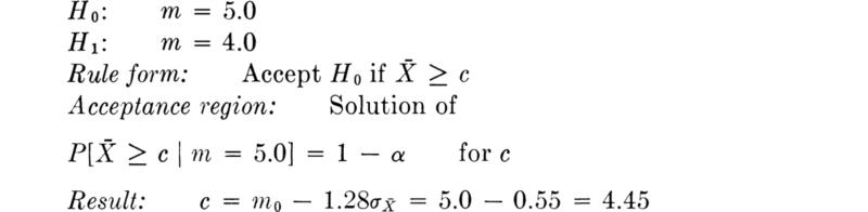
Notice that the logical form of the operating rule has changed to reflect the engineer’s belief that m is either 5.0 or a smaller value (namely, 4.0). Such a test is called one-sided, as compared with the previous example, which was a two-sided test. Notice, too, that the alternate hypothesis H1 is a simple hypothesis, meaning only a single value of m is associated with the hypothesis. In contrast, in the previous example, H1 was m ≠ 5.0, which is called a composite hypothesis in that it is composed of a collection of values of m, in this case infinitely many. One implication of having a simple alternate hypothesis is that there is a unique value for β, the type II error probability. In this case the probability of incorrectly accepting H0 when H1 is true is simply
Consider another case where the engineer must report only that the mean is above a certain value m0 or below it. For example, if the materials engineer represents the state highway department, he might guard only against too small quantities of asphalt content; he is not responsible for identifying excessive asphalt content, which is uneconomical to the supplier. The hypothesis test in this case would logically be:
Notice that there is no unique solution for c since H0 is now a composite hypothesis. There is a different value of c for each value of m equal to or greater than 5.0. In practice c would be chosen so that α is no more than 10 percent. In this case the implication is solving for c when m is set equal to the smallest value permitted by H0, namely, 5.0. The result is: c = 4.45 just as in the previous example where H0 and H1 were both simple hypotheses.
The use of other statistics in the test The sample mean, ![]() has been used above in hypothesis tests concerning the true mean m. It should be emphasized that other sample statistics may, for a variety of reasons, be more appropriate. For example, if the underlying variable X is normally distributed, N (m,σ2), but neither m nor σ is known, it is desirable to work with the “t statistic” if the sample size is small. This statistic was also used in similar circumstances to obtain a confidence-interval estimate† of m in Sec. 4.1.3. Consider again the original asphalt-content example. If the materials engineer were not confident of the value of σ2, owing, say, to a limited experience with the plant setup, he should use the following test, involving an estimator of σ:
has been used above in hypothesis tests concerning the true mean m. It should be emphasized that other sample statistics may, for a variety of reasons, be more appropriate. For example, if the underlying variable X is normally distributed, N (m,σ2), but neither m nor σ is known, it is desirable to work with the “t statistic” if the sample size is small. This statistic was also used in similar circumstances to obtain a confidence-interval estimate† of m in Sec. 4.1.3. Consider again the original asphalt-content example. If the materials engineer were not confident of the value of σ2, owing, say, to a limited experience with the plant setup, he should use the following test, involving an estimator of σ:
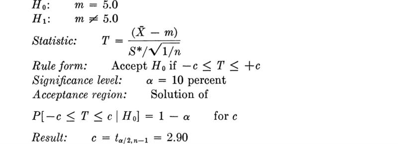
Recall (Sec. 4.1.3) that (S*)2 = S2* is the unbiased estimate of σ2 and tα/2,n–1 is the value from a table of the t statistic (Table A.3) which a t-distributed random variable with n – 1 degrees of freedom (in this case, n – 1 = 3 – 1 = 2) will exceed with probability α/2.
With the same observations of asphalt content obtained in the previous example, namely, x1 = 4.2, x2 = 4.7, and x3 = 3.7, the sample mean is ![]() = 4.2, and
= 4.2, and

Thus, given H0 or m = 5, the observed t statistic is

Since this value is between ±2.90, the null hypothesis should be accepted at the 10 percent level. Notice that this is in contrast to the conclusion of rejection suggested by the original test. The change in conclusion results (despite the fact that the observed value of S* is considerably smaller than the previously given value of σ = 0.75) from the fact that the “allowance for” uncertainty in σ implied by the use of the t statistic leads to wider acceptance regions when the sample size is small. (Compare tα/2,n–1 = 2.90 for a/2 = 5 percent and n – 1 = 2 with the value from a normal table of kα/2 = 1 .64 for α/2 = 5 percent.)
In quality-control practice it is common to use other, more easily calculated sample statistics in routine hypothesis testing. Simply to avoid calculation in the field of the sample average, the engineer might have set up the following test in one of the examples above:
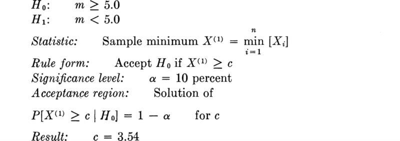
Again assuming that σ is known to equal 0.75 and using the smallest value of m permitted by the composite hypothesis H0 (namely, m= 5), c is found simply by

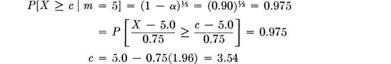
With the data obtained, 4.2, 4.7, and 3.7, the null hypothesis should be accepted since the minimum value, 3.7, is greater than 3.54.
In principle, when considering two different test forms, such as those above involving either ![]() or X(1), the sample mean or the sample minimum, one should study the behavior of the type II errors in detail. For a fixed value of α, one would like a test whose β probabilities are smaller than those for all other tests (at the same significance level); that is, a test with an OC curve below the OC curves of other tests under consideration. Such a test, if it can be found, is said to be the most powerful test.† Such comparative studies are usually left to mathematical statisticians, who recommend the most appropriate tests. In routine testing, the civil engineer must, however, be prepared to balance a loss in test power versus a simplification of the application of the test in the field. For this reason, many quality-control specifications are written in terms such as “accept the material if no more than 2 of 10 samples fail to meet the prescribed level (of strength, say),” rather than in terms of sample averages and variances.
or X(1), the sample mean or the sample minimum, one should study the behavior of the type II errors in detail. For a fixed value of α, one would like a test whose β probabilities are smaller than those for all other tests (at the same significance level); that is, a test with an OC curve below the OC curves of other tests under consideration. Such a test, if it can be found, is said to be the most powerful test.† Such comparative studies are usually left to mathematical statisticians, who recommend the most appropriate tests. In routine testing, the civil engineer must, however, be prepared to balance a loss in test power versus a simplification of the application of the test in the field. For this reason, many quality-control specifications are written in terms such as “accept the material if no more than 2 of 10 samples fail to meet the prescribed level (of strength, say),” rather than in terms of sample averages and variances.
Tests on dispersion Suppose that a development engineer is interested in the influence of a new earth-moving device on construction projects. Dispersion in haul times is known to cause idle equipment and long queues. On a particular job, the present equipment has a variance in haul times of σ02. The new equipment is to be tested for a short time. The engineer must report whether there is a reduction in σ2. He must attempt to abstract significance from the limited trial data as to whether there has been a change. His test might be:
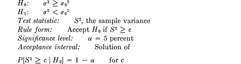
If the underlying individual times are normally distributed, then the distribution of S2 is related to the χ2 distribution (Sec. 4.1.3), and c can be easily found for any particular sample size, with σ2 set equal to σ02, the lowest value permitted by H0.
Notice that there is freedom for the engineer to choose whether H0 be σ 2 ≥ σ02 or σ2 ≤ σ02. The form of the test will be different, the type II errors will be different, and even the conclusions from the same data may be different. In the first case the engineer knows that the (maximum) probability of saying that σ2 < σ02 when it is not is 5 percent, whereas in the second case, the engineer knows that the (maximum) probability of concluding that σ2 > σ02 when it is not is 5 percent. Which choice is appropriate depends in principle upon the consequences implicit with each kind of error. In practice, a conventional value of α is used and the engineer chooses H0 to be σ 2 ≥ σ02 or σ2 ≤ σ02, depending upon the position he wants to bias himself toward. For example, if the equipment-development engineer felt that he should be conservative and not suggest that the device was better (i.e., that it had σ2 smaller than σ02) unless he were quite sure, then he should set H0 as σ2 > σ02; that is, he should assume that the new device is worse unless the data is significantly contradictory and “forces” him to reject the hypothesis. On the other hand, if the engineer is convinced that the new device is better and he seeks only supporting evidence, he might set H0 as σ2 < σ02; that is, he might assume that it is better unless the data deviates significantly from the expectation and forces him to reject that assumption. A similar duality exists in statistical quality control. The organization which must accept the material will usually assume that the mean material property (say, strength) is less than some fixed value unless the data indicate that it is “significantly” above. This encourages the supplier to produce material with low variance and to provide large samples. In routinely controlling the output of his own plant, however, the producer may assume that the mean is above some fixed value unless the samples are significantly low to cause him to take expensive corrective action. The difference in attitude will appear in the choice of the null hypothesis.
In routine testing, the sample range (maximum observation minus minimum observation) is sometimes used as the test statistic when considering dispersion. It is trivial to calculate in the field, and its distribution has been tabulated, at least for normal variables (e.g., Burlington and May [1953]).
Tests on two sets of data In certain situations the engineer may want to look at two sets of data, x1, x2, . . ., xn, and y1, y2, . . ., yr, and decide if one set comes from the same population as the other or if one set represents data from a sample with a higher mean than the other. The data from one set may represent durability tests on concrete with a new additive designed to increase workability. The other data represent the control group, one which is treated in all ways in a similar manner, but which lacks the additive.
If the variances of X and Y are known, the test statistic usually used is the difference in the sample means,![]() . If X and Y are normal, then
. If X and Y are normal, then ![]() is normal with mean mX – mY and variance (σx2/n + σY2/r. Therefore, one might, for example, set up a one-sided test:
is normal with mean mX – mY and variance (σx2/n + σY2/r. Therefore, one might, for example, set up a one-sided test:
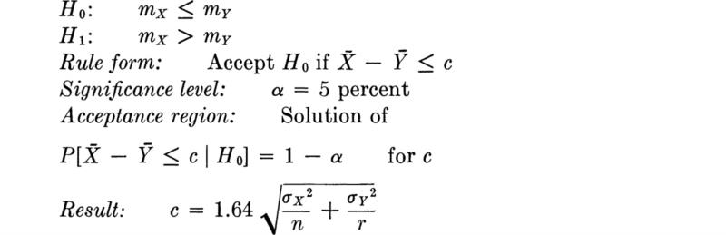
There exist many kinds and forms for tests involving the means of two variables. Some of these are “nonparametric,” meaning that the distribution of X and Y need not be assumed. The reader is referred to standard statistics texts for their enumeration (e.g., Hald [1952], Bowker and Lieberman [1959], or Freeman [1963]).
Another test involving two populations is that which tests for equality of the two variances (or standard deviations). The test statistic used if the variables are both normal is the ratio of the unbiased sample variances:
The statistic has a widely tabulated distribution, the so-called F distribution (Sec. 3.4.3), if the null hypothesis, σX2 = σY2, holds. In that case

The former ratio is the ratio of two χ2 random variables, ![]() and
and ![]() , divided by their degrees of freedom, n – 1 and r – 1. As discussed in Sec. 3.4.3, this random variable has two parameters, n – 1 and r – 1. A typical one-sided test would be of the form:
, divided by their degrees of freedom, n – 1 and r – 1. As discussed in Sec. 3.4.3, this random variable has two parameters, n – 1 and r – 1. A typical one-sided test would be of the form:
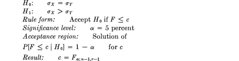
in which Fα;n–1,r–1 is that value (found in Table A.6) which an F-distributed random variable with n – 1 and r – 1 degrees of freedom will exceed only with probability a.
A final test we will mention involving two random variables is a test for lack of correlation, that is ρX,Y = 0. If X and Y are jointly normally distributed, it can be shown that the sample correlation coefficient (Sec. 1.3)
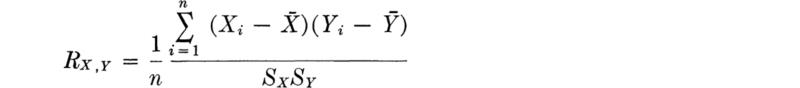
has a distribution related to the t distribution with n – 2 degrees of freedom under the null hypothesis H0 that ρ = 0. If ρ ≠ 0, the distribution of R is complicated even for X and Y jointly normal.†
In the joint normal case this becomes a test for independence of the following form:
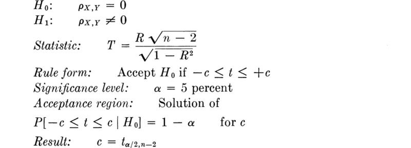
For example, using the beam-crack and ultimate-load data of Sec. 1.3, Table 1.2.2, the sample correlation coefficient of 15 specimens was found to be 0.12. If the loads are assumed to be normally distributed, the research engineer could report that at the 5 percent significance level the crack load and ultimate load were found to be independent, since

This value is between ±2.160, the range from Table A.3 beyond which a t variable with 13 degrees of freedom will be 5 percent of the time.
Discussion The method of hypothesis testing provides the service of extracting significance from data, but it suffers from several limitations with respect to arbitrariness in selecting significance levels and forms of hypotheses. In practice, engineers will sometimes beg the question of significance level by reporting only that significance level at which the hypothesis would have to be rejected given the observed value of the statistic. For example, in the original example in Sec. 4.2.1, the observed value of, ![]() was
was ![]() = 4.2. This value lies
= 4.2. This value lies ![]() standard deviations,
standard deviations, ![]() , below the expected value of
, below the expected value of ![]() (given the null hypothesis). Therefore the hypothesis would have to be rejected at all significance levels greater than 6.2 percent. This value is sometimes called the p level of the test.
(given the null hypothesis). Therefore the hypothesis would have to be rejected at all significance levels greater than 6.2 percent. This value is sometimes called the p level of the test.
In any case the method of hypothesis testing provides a convenient, conventional method for reporting the basis on which a conclusion was reached in the light of scatter in the data. The reader of such a report must retain, however, his critical attitude, in the broad sense of the word. On the basis of the report, he knows how the conclusion was reached, and he must judge the conclusion in the face of known limitations in the method. For the engineer, the necessity for choosing somewhat arbitrarily among conventional values of significance levels and among forms of hypotheses will often prove unsatisfactory. In many such situations, more powerful tools for decision making in the face of uncertainty (Chaps. 5 and 6) should be considered instead.
A conventional method for “extracting significance” from disperse data has been presented in brief. Hypothesis testing is an aid in verifying certain assumptions that the engineer might make about his model. Described here are various tests on assumptions about model parameters. The procedure requires that the engineer state two exclusive hypotheses–H0, the null hypothesis, and H1 the alternate hypothesis. Based on a chosen sample statistic to be used in the test, the appropriate form of the operating rule is selected. Given a prescribed value for α, which is the probability of the type I error (rejecting H0 when it is true), an acceptance region (or, its complement, the critical region) is calculated in the sample space of the sample statistic such that there is a probability of 1– α that the sample statistic will lie in the acceptance region, given that H0 holds.
The hypothesis test is run by obtaining the data, calculating the observed statistic, and comparing it with acceptance region. The engineer will state that “H0 is accepted at the α significance level” if the observed statistic lies in the range. The observed statistic is said to be significant if it lies in the critical region, suggesting that the null hypothesis is not true.
In principle, the user must also consider for any test the probability β of a type II error (accepting H0 when it is not true). If H1 is a composite hypothesis, it is necessary to plot β versus all possible values of the true parameter permitted by this hypothesis. Such a plot is called an operating characteristic (OC) curve for the test.
A number of examples showed one-sided and two-sided tests, simple and composite hypotheses, and cases involving means, variances, and correlation coefficients as parameters of one or two sets of data.
As in mechanics, linear models of physical phenomena are widely used in applied probability and statistics. In this case, by a linear model it is meant that a random variable Y is affected in its mean in a linear manner by another variable x or variables, x1, x2, . . ., xr. The other variables may or may not be random. The underlying model says that E[Y | x1,x2, . . . ,xr] = α + β1x1 + β2x2 + · · · + ·r. In this section we will provide a brief, introductory look at the formulation and the statistical analysis of such linear models. By statistical analysis we mean parameter estimation and significance testing. We shall ask such questions as, “What are estimates of the βi’s?” and “Is the observed dependence of the mean of Y on xj statistically significant?” Much of this statistical analysis falls under the customary title of regression analysis. In one sense we will simply be applying the tools of Secs. 4.1 and 4.2 to a very useful new class of models.
A wide variety of practical problems can be represented by linear models. In this section we shall discuss the characteristics of some of these probability models, concentrating on the simpler cases but indicating the extensions to other problems. The section ends with a discussion of the statistical interests we should have in such models. In Sec. 4.3.2, we shall demonstrate the statistical analysis of the simpler cases.
Model 1 In the simplest case a linear model states that the mean of the random variable Y is linearly functionally dependent on x, which is a nonrandom quantity but one which may change from experiment to experiment. Let us denote this by saying
In any single experiment x will have some value xi, and the expected value of Yi will be α + βxi. Yi itself can be written
in which Ei is mean zero random variable, sometimes called the ” error term.”
Consider some examples. In a particular deep layer of soil, the soil will be sampled at a number of depths, x1, x2, . . ., xn. The sample will be recovered and tested. It may be reasonable to assume that the expected value of Yi the unconfined compressive strength at depth xi is α + βxi. The basic assumption of the model is that within this geological layer there is a general linear trend in the strength with depth. Owing to small-scale local soil variations and due to sampling and testing variability, † the observed unconfined compressive strengths will show scatter or dispersion about this trend; that is, Yi is a random variable with mean α + βxi, with some variance σi2, and some distribution ![]() . (In much of the statistical analysis to follow we will make the specific assumptions that σ2 does not depend on xi and that
. (In much of the statistical analysis to follow we will make the specific assumptions that σ2 does not depend on xi and that ![]() is normal.) Figure 4.3.1 shows observed data that may follow this model. Note that if the slope β were zero, the model would simply be that soil strength throughout the layer is a random variable Y. In this case, the problem analysis would simply follow that discussed in previous sections of the text.
is normal.) Figure 4.3.1 shows observed data that may follow this model. Note that if the slope β were zero, the model would simply be that soil strength throughout the layer is a random variable Y. In this case, the problem analysis would simply follow that discussed in previous sections of the text.
In studying the growth of strength of concrete with age x at low curing temperatures, it is reasonable to assume that the mean compressive strength Y grows linearly with age during the initial curing period, when form removal might be contemplated. Individual cylinders strengths are random variables with some distribution about this mean.
In this so-called model 1, it is important to recognize that the x’s are not random variables, but values selected by the engineer prior to carrying out the experiment.
Fig. 4.3.1 Scattergram of data for simple (model 1) linear model analysis. Unconfined compressive strength versus depth.
Model 2 In this class of linear models interest focuses on prediction– prediction of one random variable Y given an observation of another random variable X (or others X1, X2, . . ., Xr). The linear model states that the conditional expected value of Y given X = x (see Sec. 2.4.3) is a linear function of x:
or, more simply, in this chapter we use the notation
Conditional on the value x of X, the random variable Y has some (conditional) distribution about this mean and some (conditional) variance σ2. In much of the statistical analysis to follow, it is assumed that this conditional distribution is normal with a variance not dependent on the specific value x. We have already seen one case in which all of these assumptions hold, namely, that in which X and Y are jointly normally distributed, Sec. 3.6.2. If X and Y are jointly normal, recall that
which is of the linear form assumed above with
and
mY, mX, σY, and σX are the marginal means and standard deviations of Y and X.
Again it is sometimes convenient to write that, conditional on X = xi, Y can be written
in which Ei is a random variable distributed exactly like Yi except that it has zero mean. Notice that if it is assumed (as we shall later) that for any xi, Yi is normal with mean α + βxi and with the same variance σ2, then we are assuming that the Ei are identically distributed, N(0,σ2).
Examples of these prediction problems include the following. For a system of soil-embankment flood levees, engineers in charge of design, construction, and maintenance want to be able to judge in-place shear strengths quickly and economically over wide areas. To do so they will use a simple field-shear-vane test. Because most design methods and experience are related to shear strengths determined from unconfined compressive tests, it is necessary to predict this latter strength index Y given an observed value of the field-vane test X. Both these quantities are random owing to spatial material variation and to testing variability. The analytical model adopted says that, given a field-vane value x at a particular point, the expected value of the conventional shear strength measure Y is α + βx. In a sense the model represents a probabilistic calibration of the field test.
Similarly, an engineer might assume that the total rainfall on a watershed in a particular month Y is a random variable whose conditional mean is α + βx, given that a rainfall of X = x was observed in the preceding month. In developing a highway user’s-cost model, an engineer has assumed that the user’s total maintenance cost Y can be predicted from his total fuel cost X in the sense that the expected value of Y, given X = x, is α + βx. Both X and Y, of course, vary from user to user.
The fact that both X and Y are random variables implies that, if appropriate, the engineer could consider the alternate but analogous prediction problem, ![]() . Whether this is appropriate depends upon how the model will be used in practice. That is, will the engineer predict X given Y = y or F given X = x, (the rainfall in month k given rainfall in month k + 1 or vice versa) ? It also depends upon whether the linearity assumption remains valid. One case in which it does is when X and Y are jointly normally distributed, when
. Whether this is appropriate depends upon how the model will be used in practice. That is, will the engineer predict X given Y = y or F given X = x, (the rainfall in month k given rainfall in month k + 1 or vice versa) ? It also depends upon whether the linearity assumption remains valid. One case in which it does is when X and Y are jointly normally distributed, when
Notice that in general this equation would not represent the same line on a plot of y versus x as ![]() , Eq. (4.3.5). The slope of y on x in the latter case, for instance, is
, Eq. (4.3.5). The slope of y on x in the latter case, for instance, is![]() , while in the former case it is
, while in the former case it is ![]() . The two slopes are the same only if ρ = 1, which holds only if there is no scatter (of probability mass or of observed data) about the line. In general the two (regression) lines do pass through mX and mY) however.
. The two slopes are the same only if ρ = 1, which holds only if there is no scatter (of probability mass or of observed data) about the line. In general the two (regression) lines do pass through mX and mY) however.
The distinction between model 1 and model 2 lies in the interpretation of x, whether it represents an essentially preselected value (measured without error) or whether it represents the observed value of a random variable X. In either case the fundamental assumption of a linear model is, for a given number x, that the expected value of Y is linear in x, α + βx. Virtually none of the statistical analysis which follows distinguishes between the two models, but the distinction in interpretation is fundamental to the engineering user.
Statistical questions From a set of n experiments the engineer will have n pairs of observations {yi,xi}, i = 1, 2, . . ., n, such as those represented by points in Fig. 4.3.1. As with the simple models discussed in previous sections, the statistical analysis of a linear model involves two kinds of questions, estimation of parameters and verification of model assumptions. In the simplest model we generally have three parameters to estimate: the intercept α, the slope β, and the variance term σ2. We shall be interested in finding estimators for these parameters. As before, we shall study the probabilistic behavior of these estimators in order to quantify the uncertainty we have in the parameter estimates. In addition we shall want to express the uncertainty we have in an estimate of the mean of Y, E[Y]x = α + βx for any value of x. For example, consider the engineer dealing with the soil strength versus depth problem mentioned above. He has been asked for, as input to a stability-analysis computation, the spatial average of the soil strength over a horizontal strip of finite thickness. For the linear assumption adopted here, this spatial average is simply the value of the mean of Y at xg, the mid-depth of the strip, α + βx. The engineer might choose to report both his best estimate of α + βxg and, as a “conservative” estimate of α + βxg, the 95 percent lower confidence limit on α + βxg.
A number of important questions about the model can be asked. Among the most important is whether the data indicate a significant dependence of the mean of Y on x. Formally, we consider the null hypothesis H0 that (β = 0. If there is no dependence,† the model can be simplified by ignoring x and treating Y as a simple random variable. The implication in the soil strength versus depth example is that the strength is independent of depth. In a model 2 situation, such as the example of rainfall in two successive months, the implication of no (linear) dependence of the conditional means of Y on x is that Y and X are uncorrelated [e.g., see Eq. (4.3.5)]. In a calibration situation like that of vane test versus lab test of shear strength mentioned above, the engineer might want to determine whether the estimated value of the intercept α is significantly different from zero. If not, again the model could be simplified, now to E[Y]x = βx. The engineer in this situation might want to know, too, if β is unity. If E[Y]x = x, then the vane test is a direct, unbiased predictor of the lab index of strength.
We shall analyze these estimation and statistical-significance questions in Sec. 4.3.2.
It should be pointed out that in the case of model 2, with both X and Y random, it would be equally appropriate to estimate from the data the five customary parameters, mX, mY, σX, σY, and ρ. This is called statistical correlation analysis, which is distinct from the regression or prediction analysis we have been considering. Correlation analysis has the property that it is “symmetrical” in the two variables X and Y. Regression, on the other hand, is directly concerned with what may be the ultimate application, namely, one or the other of the prediction equations,![]() . These equations are not symmetrical, as discussed above. We shall find in Sec. 4.3.2, however, that there is a close relationship between the two kinds of statistical analyses.
. These equations are not symmetrical, as discussed above. We shall find in Sec. 4.3.2, however, that there is a close relationship between the two kinds of statistical analyses.
Extensions Although their statistical analysis is beyond the scope of this text, it is worthwhile to point out extensions of the simple linear probability models mentioned above. The reader is referred to any of many texts that discuss the problems of estimation and hypothesis testing surrounding these models (e.g., Freeman [1963], Hald [1952], Brownlee [1965], or Graybill [1961]).
Transformations The easiest extension is to note that x can represent some transformation or function of the variable of interest. For example, in the concrete-strength-versus-age example above the relationship
E[Y]x = α + β In (age) might be more appropriate at higher curing temperatures. If we define x = In (age), then the model reverts to the linear form. Also, suppose that the relationship between the dependent variable Z and the independent† variable w is
in which Q is a random factor. Then, by taking logarithms, we obtain
![]()
Defining Y = In Z, α = In α', x = In w, and E = In Q, we again obtain a linear model like that in Eq. (4.3.2). It must be cautioned that any assumptions about normality or about independence of σ with respect to x adopted in the statistical analysis of the model must be made on E or In Q, not on Q itself. With this warning the analysis methods in Sec. 4.3.2 can also be used for these transformed problems. The analysis requires, in fact, only linearity in the relationship between E[Y]x and the parameters α and β
Multivariate extensions More interesting extensions involve the introduction of an arbitrary number of independent variables x1, x2, . . ., xr so that the model becomes
in which the symbol x implies that the values x1, x2,. . ., xr, a vector of variables, are specified. With this model (for r = 3) the soils engineer could study trends in the soil strength in a particular geological layer under an entire dam site, in two plan dimensions as well as in depth. Similarly, the engineer investigating “persistence” in monthly rainfall could assume that rainfall in the next month depends, in the mean, on the past r months.
In both cases (the first a model 1 and the second a model 2), the engineer has observed data {yi,, xi1 ,xi2, . . . ,xir}, for i = 1 to n, the sample size. He is interested in estimating α, the βj’s (j = 1, 2, . . ., r), and σ2, the (usually assumed constant) variance of Y given the xj values. Questions of major interest would include whether the value of any particular βj or the values of any particular subset of the βj’s were zero. For example, do the data indicate a significant dependence of the mean soil strength on the direction x2, perpendicular to the dam’s axis? And is the expected rainfall in the next month significantly dependent on months more than 1 month in the past (i.e., are the βj = 0 for all j ≥ 2)?
All fields in civil engineering have made use of such multivariate models† and their statistical analysis. The method is usually referred to as multiple-regression analysis. It should be pointed out that with multiple independent variables it is possible to construct models which are best interpreted as a mixture of model 1 and model 2. For example, the study of lab shear-strength prediction of soil might be enhanced if the engineers asked for the expected value of this strength given the field-vane-test observation x1 and the sample depth x2. The first of these independent variables is the observed value of a random variable X1, and the second is of the preselected, nonrandom kind.
If all the independent variables are of the model 2 type, then Y and the Xj’s are, in fact, r + 1 jointly distributed random variables.‡ It is appropriate in such cases to carry out a correlation analysis to estimate means, variances, and an array of pairwise correlation coefficients. In addition, correlation analysis may include computation of partial correlation coefficients, which in the multivariate normal case represent the correlation coefficient of the conditional distribution of Y and Xk, given that some partial set of the Xj’s have taken on fixed (but unspecified) values. § These coefficients and correlation analysis can be of major value in the study of such multivariate problems, but we shall not pursue them further. See, for example, Graybill [1961].
Extensions: Analysis of variance We shall consider one further extension or interpretation of linear models. It will serve to indicate another class of problems open to this kind of statistical analysis. The original simple model assumed that the mean of Y was a continuous linear function of a single continuous variable x. Suppose now that the independent quantity upon which the mean of Y depends is discrete and nonquantitative, perhaps not even amenable to any kind of ordering. For example, suppose an engineer would like to study the expected traffic demand between center city and suburbs as a function of the socioeconomic class (high, middle, or low) of suburbs. The linear model is usually written
in which βk is factor which depends on suburb class (k = 1, high; k = 2,
middle; k = 3, low), and in which a is selected such that β1 + β2 + β3 = 0. We note with interest that the model can be considered as familiar linear regression model if we consider three variables x1, x2 and x3,
with x1, x2, and x3 defined such that for, say, a middle-class suburb, x1 = 0, x2 = 1, and x3 = 0. Only one of the three xi’s is nonzero at a time; if nonzero, its value is 1.
Again the statistical analysis begins with sets of data and seeks parameter estimates and answers to model verification or statistical-significance questions. In the example above, the engineer would like to know if the parameter estimates β1, β2, and β3 are significantly different from zero. That is, does socioeconomic class have any influence on traffic demand?
Notice that two (or more) factors may be involved in a model of this kind. For example, in a study of beach erosion prevention, a research engineer may select four different types of protective material and three different shapes of the beach profile for test in a small-scale physical model with a wave generator. If Y represents a measure of erosion rate, the analytical model might be
![]()
The β’s are associated here with material types and the τ’s with shape types. In regression form, the model is
in which for any test only one of x1, x2, x3 or x4 will be unity, depending on the protective material, and only one of x5, x6, and x7 will be unity, depending on the beach shape. It is important to recognize that, contrary to common belief, one can make statements about, say, the significance of the beach shape (i.e., are β5, β6, and β7 all zero?) without testing all 12 possible combinations of protective material and shape. Recognition of this fact can reduce the cost of physical experiments. In this example, the engineer might believe, in addition, that there exists the possibility of “interaction” between the material and the beach shape, that is, that material 1 is more effective on a convex shape than on a concave one, whereas material 2 may be just the reverse. A model including interaction is normally written
in which the γkj are the 12 so-called “interaction terms,” one of which acts when the material is the kth type and the shape the jth type. In regression form, the model becomes
in which there are (3×4=) 12 additional parameters βl, l = 8, 9, . . ., 19, one for each combination of material and shape, xk and xj. Note that xj and xk being restricted to (0,1) variables implies that their product is unity if and only if they are both acting. Important hypothesis tests would now include questions with respect to the values of the interaction parameters βl. In particular, “Are they zero?”
The kind of model we have just been discussing, that with discrete levels for the independent variables, is customarily given its hypothesis-testing analysis under the title analysis of variance or design of experiments, † The interpretation given there is that various “treatments” (e.g., the beach shape or the beach protection material) contribute various components to the total variance of Y. Analysis of the components leads to tests (F tests) on the significance of any treatment, or interaction between treatments. The regression formulation has the advantage of uniformity ‡ in appearance and treatment, and there exist widely available computer programs for performing the numerical analysis.
Having discussed the formulation of a wide variety of linear models, we turn now to demonstrate the statistical analysis of the simplest such model:
We consider first parameter estimation and then significance testing. Additional assumptions about the properties of the linear model will be introduced as necessary.
Point estimates of parameters Any of a variety of parameter estimators, ![]() and
and ![]() could be considered; these estimators are usually obtained by the least squares method.§ This method states that
could be considered; these estimators are usually obtained by the least squares method.§ This method states that ![]() and
and ![]() be chosen to minimize the sum of the squared differences between the observed values
be chosen to minimize the sum of the squared differences between the observed values
Fig. 4.3.2 The residual, or the “vertical” distance between yi and the estimated line, ![]() .
.
yi and the estimated expected values ![]() that is, one should choose
that is, one should choose ![]() and
and ![]() to minimize
to minimize
As shown in Fig. 4.3.2, these differences, called the residuals, are the “vertical” distances between the yi and an estimate ![]() of the true line α+βx.
of the true line α+βx.
To find the estimates of ![]() and
and ![]() , we simply take partial derivatives of the sum of squares expression with respect to
, we simply take partial derivatives of the sum of squares expression with respect to ![]() and
and ![]() , set these two derivatives equal to zero, and solve for the
, set these two derivatives equal to zero, and solve for the ![]() and
and ![]() which minimize the sum. Thus
which minimize the sum. Thus
and
Carrying out the summations and simplifying yields two simultaneous linear equations in ![]() and
and ![]() :
:
in which ȳ is the average of the yi’s, (l/n)∑yi, and ![]() is the average of the xi’s 1/n)∑xi.
is the average of the xi’s 1/n)∑xi.
Solution of these, the so-called normal equations, is trivial.
Using Eqs. (1.2.2b) and (1.3.2) (also see Prob. 1.19), it is clear that we can also write †
in which SX,Y is the sample covariance, rX,Y is the sample correlation coefficient, and sX and sY are the sample standard deviations, all defined in Chap. 1.
Example Consider the data in Fig. 4.3.3 of yi's, the true, lab-measured water content in randomly selected field soil specimens from a particular site, and the corresponding xi’s, the water content estimated by a fast, inexpensive method which measures the gas pressure created when the soil is mixed with a chemical which reacts with water. If it is sufficiently accurate, the second method will provide an inexpensive way to obtain more frequent water-content samples during the quality control of soil compaction on a highway project. The purpose is to predict true water content given an observed value of the fast test. This is a model 2 example.
The sample size is n = 67. The calculated values needed are
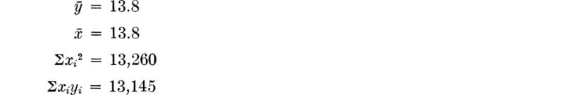
(The equality of ȳ and ![]() is coincidence.) Therefore the estimates of
is coincidence.) Therefore the estimates of ![]() and
and ![]() are
are
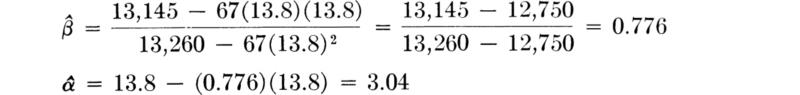
This estimated regression line is shown with the data in Fig. 4.3.3.
Also shown in the figure is an estimate, ![]() , of σ, the assumed constant standard deviation of Y given x. The obvious estimator of σ2,
, of σ, the assumed constant standard deviation of Y given x. The obvious estimator of σ2,![]() , is the average of the squared residuals. That is,
, is the average of the squared residuals. That is,
Fig. 4.3.3 Scattergram of water-content data showing estimated regression line.
which upon substitution for ![]() and
and ![]() can be reduced for ease in computation to†
can be reduced for ease in computation to†
Note the use of a divisor of n – 2 rather than n in Eq. (4.3.26). This is customary, since it can be shown to produce an unbiased estimator of σ2.
In our example (with ∑yi2 = 13,291),
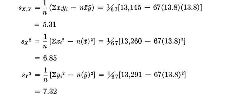
implying

Thus
![]()
and
![]()
This completes the process of obtaining point estimates of the model parameters, α, β, and σ2.
Properties of estimators In order to determine confidence intervals or to carry out significance tests we must, as in Sec. 4.1, study the properties of the estimators as random variables. This requires adopting a position prior‡ to the experiment, when the Yi’s are random variables, and determining the mean, variance, and distribution of these estimators as functions of the Yi’s. We shall demonstrate one case only, and simply state readily verifiable conclusions for others.
Consider the estimator of the slope, ![]() Emphasizing its character prior to the experiment as a random variable, we write it as B. Then, from Eq. (4.3.24),
Emphasizing its character prior to the experiment as a random variable, we write it as B. Then, from Eq. (4.3.24),
The xi’s are all known constants. The Yi’s and Ῡ are random variables. The numerator of B can be expanded to
in which ci = ![]() . The purpose of the expansion is to recognize the important fact that B, the least squares estimator of β, is a linear combination of the Yi’s As we have seen, this simplifies analysis greatly. For example, the expected value of B is quickly found to be
. The purpose of the expansion is to recognize the important fact that B, the least squares estimator of β, is a linear combination of the Yi’s As we have seen, this simplifies analysis greatly. For example, the expected value of B is quickly found to be
since ∑ci = 0 and ∑cixi = 1. The implication is that B is an unbiased estimator of β.
Similarly, if we now make the assumption that the Yi’s are uncorrelated, e.g., if we have a random sample,† then
If we also assume now that the Yi’s have the same variance σ2, no matter what xi is, then
Note the characteristic decay in an estimator’s variance (like 1/n) and note that, if, as in a model 1 situation, the engineer is able to preselect the xi’s, he can reduce the uncertainty in the slope by spreading the xi’s as much as possible to increase sX2.
With a large enough sample size, we could safely assume (by the central limit theorem) that B is approximately normally distributed, no matter how the Yi are distributed. With this information, and with an estimate s2 for σ2, we could prepare confidence limits on β. For example, 1 – α two-sided confidence interval would be
![]()
in which kα/2 is taken from a normal table (Sec. 4.1). For smaller sample sizes, we must adopt a distribution for the Yi’s. If we assume that the Yi’s are normal and independent, then B is also normal, since it is a linear combination of independent normal variables. But for small n and unknown σ, it should be clear from experience in Secs. 4.1 and 4.2 that such confidence intervals must be based on a value from a table of the t distribution, tα/2,n–2, and sB, the estimate of σB based on replacing σ by its estimate s in Eq. (4.3.32). The confidence interval is then
Note that the n – 2 degrees of freedom are used in entering the t table (A.3).
In the example just considered

implying that a 90 percent confidence interval on the true slope β is
![]()
or
![]()
(Assuming B normal would have replaced 1.67 by 1.64, i.e., t0.05, 65 by k0.05.)
Without proof, it is easily shown that A is also a linear combination of the Yi’s, that it is an unbiased estimator of α, and that its variance is
In our example, the estimate of σA is

The 90 percent confidence intervals are also based on a t distribution:
or
![]()
Under the same assumptions the estimator S2 of σ2 is unbiased with a distribution related to the χ2 distribution. Specifically,
is χ2-distributed with n – 2 degrees of freedom. Therefore, for example, a 90 percent one-sided lower confidence interval on σ2 is found from the statement (Sec. 4.1)

which implies that

The lower limit in our example is

As a final example we can find the properties of the estimator of E[Y]x = α+ βx for any particular x, say x0. Calling this estimator ![]() , we can find that it, too, is a linear combination of the Yi’s with mean
, we can find that it, too, is a linear combination of the Yi’s with mean
![]()
and variance
Note that the variance depends on x0. At x0 equal to ![]() , that is, near the middle of the data,
, that is, near the middle of the data, ![]() is equal to simply σ2/n, while for values of x0 removed from
is equal to simply σ2/n, while for values of x0 removed from ![]() , for example, near the extremes of the data, the variance in the estimator of
, for example, near the extremes of the data, the variance in the estimator of ![]() grows. Note that for
grows. Note that for ![]() equals the variance of A, the estimator of the intercept, as it should.
equals the variance of A, the estimator of the intercept, as it should.
In our example, for a rapid water-content test value of x0 = 15, the best estimate of the expected value of Y, the true water content, is
![]()
The 90 percent confidence limits on this conditional mean are
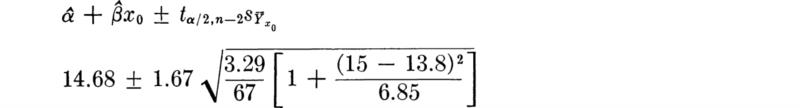
or
![]()
Fig. 4.3.4 Estimated regression line and 90 percent confidence limits on ![]() Water-content illustration.
Water-content illustration.
This value and the locus of such confidence limits for a range of values of x0 are shown in Fig. 4.3.4.
It should be emphasized that this confidence interval is on the mean of Y given x0, not on Y itself; that is, in our example, the confidence interval is on the average true water content of many soil specimens whose estimated water contents are all 15. If the engineer wants to make some kind of statement about the true water content Y of an individual specimen with an estimated water content of x = 15, he must also allow for the inherent variation σ2 about the mean value. In most texts, it is suggested that one also consider this wider interval as a confidence interval, now on Y, a single future value. It is found by simply replacing ![]() by
by ![]() in the expressions above for confidence intervals on
in the expressions above for confidence intervals on ![]() .
.
Significance tests Now that we have the distributions of the estimators, it is very easy to conduct hypothesis tests on the parameters. We demonstrate three such cases.
Suppose the engineer wants to report whether the data indicate an intercept significantly different from zero. Then we have, following the pattern in Sec. 4.2,
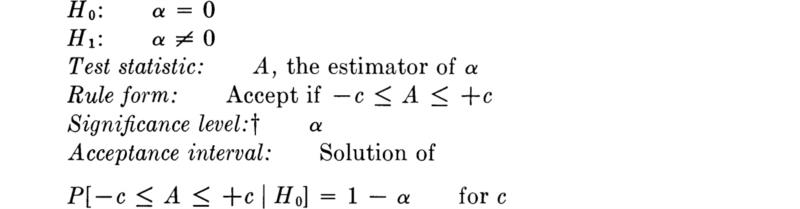
In this case we work with a t statistic and find, as expected,
For example, in the soil-water-content illustration, with α = 10 percent, we find
![]()
Since the observed value of A, ![]() , lies outside ‡ the interval ±2.00, we reject the hypothesis and state that the intercept estimate is significantly different from zero at the 10 percent significance level.
, lies outside ‡ the interval ±2.00, we reject the hypothesis and state that the intercept estimate is significantly different from zero at the 10 percent significance level.
Similarly, we could test if the slope β is, say, unity by comparing the observed value of B with the acceptance interval
![]()
(In our example, ![]() is significantly different from zero at the 10 percent level.)
is significantly different from zero at the 10 percent level.)
The most common test, however, is whether there is significant dependence of E[Y]x on x. This is tested as follows:

As above, the acceptance interval is
![]()
Note that for model 2, in which X and Y are both random, asking whether β is zero is equivalent to asking if the correlation coefficient p is zero. Compare the test on p here with that discussed in Sec. 4.2. Note that both are based on a t distribution.
For example, in the reinforced-concrete-beam data in Chap. 1, the estimate of the slope of a regression of ultimate load Y, on cracking load X, is

while
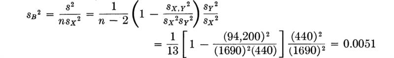
At the 10 percent significance level
![]()
The conclusion is that the slope (and the correlation coefficient) are not indicated by the data to be different from zero.
Note that all calculations involving the estimate and variance of the estimator of the slope involve only the sample variances, never the averages ![]() . As one could have predicted, a shift in the origin will not change
. As one could have predicted, a shift in the origin will not change ![]() or SB, but it will alter
or SB, but it will alter ![]() and SA. There is certain computational convenience if one shifts the origin to
and SA. There is certain computational convenience if one shifts the origin to ![]() , working then with
, working then with ![]() and
and ![]() . Two resulting simplifications, † for example, are that
. Two resulting simplifications, † for example, are that ![]() = 0 and that
= 0 and that ![]() .
.
An important class of significance tests arises when simultaneous hypotheses are tested. For example, if the engineer were considering the feasibility of reducing a model from E[Y]x = α+ βx to simply E[Y]x = x (as would be appropriate, for instance, with the water-content “calibration” example above), then in principle he should not first test {H0: α. = 0} and then {H0: β = 1}, but rather the simultaneous hypothesis
![]()
Such tests involve both estimators, A and B, and their joint distribution. In regression analysis the customary test statistic is an F-distributed variable. We shall not pursue these tests further, but we do point out their particular importance in analysis of variance problems (Sec. 4.3.1) where a multiple hypothesis such as {H0: β1 = 0, β2 = 0, and β3 = 0} is needed to test whether a particular “treatment” (e.g., socioeconomic class) has a significant influence on the dependent variable (e.g., travel demand). The reader is referred to Rao [1965], page 196, for a general treatment of simultaneous hypothesis tests in multivariate regression.
We chose not to delve into the statistical analysis of multivariate linear models. But the reader with a moderate amount of additional preparation from other texts (e.g., Hald [1952]) and with the help of the widely available computer programs for multivariate regression can find himself quickly in command of a powerful set of analytical models and data-analysis capability.
Linear models are of the general form
![]()
in which the independent variables, x1, x2, · · ·, xr, are either pre-selected nonrandom values (model 1) or observed values of random variables X1 X2, . . ., Xr (model 2). In general, interest is in predicting Y for a specified set of the xi. As such it is closely related (in the model 2 case) to linear prediction (Sec. 2.4.3) and jointly normally distributed random variables (Sec. 3.6.2) and correlation analysis.
The model can be used to represent nonlinear relationships and situations in which an independent “variable” or treatment occurs at discrete levels, possibly not even “orderable or quantifiable” (analysis of variance).
The statistical analysis of the model includes parameter estimation and significance testing. For the simplest case,
![]()
the parameter estimates are
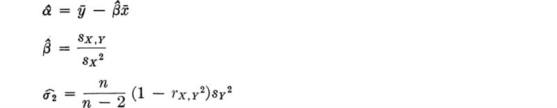
in which ![]() , and rX,Y are sample averages defined in Chap. 1, and σ2 is the (assumed constant) variance of Y about its regression line (i.e., the variance of Y given x). The estimators are linear functions of the Yi’s, and they are unbiased. Their variances are
, and rX,Y are sample averages defined in Chap. 1, and σ2 is the (assumed constant) variance of Y about its regression line (i.e., the variance of Y given x). The estimators are linear functions of the Yi’s, and they are unbiased. Their variances are
in which A and B are, respectively, ![]() and
and ![]() treated as random variables.
treated as random variables.
Confidence intervals and hypothesis tests on the parameters or functions of the parameters (for example, ![]() follow from study of the estimators’ distributions. Assuming that the Yi’s are normally distributed, t statistics are typically involved when parameters α and β are central, while the χ2 distribution governs the estimator of σ
follow from study of the estimators’ distributions. Assuming that the Yi’s are normally distributed, t statistics are typically involved when parameters α and β are central, while the χ2 distribution governs the estimator of σ
Throughout the text to this point we have always assumed that the form of the model was known—e.g., normal, Poisson, etc. In Sec. 4.1, for example, we discussed the estimation of the parameters of a given model or distribution. At the outset of the chapter, however, we recognized that a third source of uncertainty always exists, namely, that surrounding the validity of the mathematical model being proposed or hypothesized. Is it or is it not an accurate representation of the physical phenomenon? We take the position in this section that the engineer has for one reason or another adopted a mathematical model of a physical phenomenon and seeks, after gathering data, to test the validity of that particular model.
We introduce in Secs. 4.4.1 graphical ways of comparing the form of the model and that of the observed data. An understanding of the behavior of these observed shapes vis-à-vis the underlying distribution is critical to their proper interpretation. In Sec. 4.4.2, we will use this understanding to develop quantitative rules that lead to acceptance or rejection of a particular hypothesized model. In Sec. 4.5, this same understanding will underlie the discussion of the different, but related, problem of choosing from among several convenient mathematical forms the one which best fits observed data.
Observed physical data provide the engineer an opportunity to verify the model he has developed. He seeks to support or reject such statements as, “Annual floods at station A have a type II extreme value distribution,” or “Contractor B produces concrete whose compressive strength is normally distributed,” or “The traffic on highway C follows a Poisson process.”
In principle he must compare some observation with some model prediction in order to verify the validity of the latter. He could, for example, compare higher† sample moments with the corresponding moments of the mathematical model. Although occasionally such moment comparisons are useful checks, the engineer usually finds more benefit in looking at a graphical comparison of the “shapes” of the data and the model. These may deal either with a histogram of the data and a PDF (or PMF) of the model or with a cumulative histogram and a CDF. In either case the visual comparison permits an immediate assessment of the proximity of observed and predicted results and, additionally, provides information about the regions of discrepancy, if any.‡ Intuitively, such a shape comparison seems preferable to a simple higher-moment comparison in that it brings more of the information contained in the sample into the comparison and in that it tends to counter the criticism that many models may have nearly identical second- or third-order moments, but still have markedly different shapes.
Histogram versus PDF Consider the two comparisons made in Figs. 4.4.1 and 4.4.2 between the histograms and the PDF’s of the proposed models in the traffic and yield-force illustrations we considered in Sec. 4.1. Notice that the probability density functions of the models have been
Fig. 4.4.1 Bar-yield-force illustration: PDF of normal model and histogram of observed data.
Fig. 4.4.2 Traffic-interval illustration: PDF of exponential model and histogram of observed data.
shown in a bar form, coinciding with the intervals of the histograms. Owing to the grouping of data into intervals necessary to construct a histogram, it is clearly the corresponding bar form of the PDF which must be used in the comparison, and not the complete, continuous form. This requirement is unfortunate. The fine features, including the tails, of the proposed model are “smeared” and lost in the process. Narrower interval choices reduce this smearing, but at the expense of fewer observations per interval and subsequently larger fluctuations in the observed bar heights, as discussed in Chap. 1 and later in this section.
Within this restriction, however, the data seem to suggest that the traffic and yield-force models are not unreasonable. There is no apparent systematic discrepancy in the shapes, but some of the individual observed frequencies differ considerably from the predicted values. Are some of these values unduly large? Is the apparent argeement good enough? Does the engineer dare wish for a closer fit? In short, is the observed histogram shape significantly different from the predicted shape?
In order to ask such questions more precisely and to attempt to answer them, we must try to understand the histogram as well as we do the sample mean and other simple sample statistics. To achieve this end, we must, as always, assume that the model is known and then describe the probabilistic behavior of the statistics to be formed from samples taken from that model. Consider for illustration a simple triangular distribution on the interval 0 to 1, as shown in Fig. 4.4.3f. The results of several samples of size nine drawn from this distribution (using random numbers as described in Sec. 2.3.3) are shown in Fig. 4.4.3a to e. These histograms were constructed such that there was an equal probability, ![]() , of observing a value in each of the three intervals, 0 to 0.58, 0.58 to 0.82, and 0.82 to 1. The random nature of these histograms is obvious. They vary in shape from one which exaggerates the true triangular PDF (e) through one which coincides “perfectly” with the expected frequencies (b), on to bell-shaped (c), and uniform shapes (a), and to a reversed triangular shape (d). Most important for our purposes here is to consider the reaction to any one of these observed histograms that an engineer who had correctly hypothesized the underlying triangular PDF might have had. In several cases he undoubtedly would have considered the data as substantiating his proposal, but at least one (d) might have caused him (erroneously) to doubt the model.
, of observing a value in each of the three intervals, 0 to 0.58, 0.58 to 0.82, and 0.82 to 1. The random nature of these histograms is obvious. They vary in shape from one which exaggerates the true triangular PDF (e) through one which coincides “perfectly” with the expected frequencies (b), on to bell-shaped (c), and uniform shapes (a), and to a reversed triangular shape (d). Most important for our purposes here is to consider the reaction to any one of these observed histograms that an engineer who had correctly hypothesized the underlying triangular PDF might have had. In several cases he undoubtedly would have considered the data as substantiating his proposal, but at least one (d) might have caused him (erroneously) to doubt the model.
Probability law of a histogram Given the true distribution and a set of intervals, the observed histogram interval frequencies are clearly random variables that are directly proportional to the random numbers of sample observations which fall into those intervals. These numbers are jointly distributed random variables possessing a multinomial distribution (Sec. 3.6.1). If the interval probabilities are p1, p2 . . ., pk and the sample of size is n, the numbers in each interval, N1, N2, . . ., Nk, have the joint PMF [Eq. (3.6.5)]:
If the interval probabilities are equal, p1 = p2 = · · ·= pk = 1/k, a simpler result is obtained:
since n1 + n2 + · · · + nk must equal n.
Fig. 4.4.3 Five random samples from a triangular distribution, (a) Sample a; (b) sample b; (c) sample c; (d) sample d; (e) sample e; (f) true PDF and bar-form frequencies in three equally likely intervals.
With this formula we can compute the probability of obtaining any particular histogram. For example, consider the triangular distribution discussed above. For simplicity, we take k = n = 3, that is, three intervals as above, but a sample size of only three. Then the likelihood of a histogram with two observations falling in the first interval and one in the last is

Since the interval probabilities, were chosen to be equal, this probability is the same for any one of the six possible histograms with two observations in one interval and one in another. A histogram with all three observations in the same interval, say the last, has probability

The “perfect fit” is obtained only if there is a single observation in each and every interval:

The “perfect fit” is in fact always the most likely single histogram, but, as here, it is not a highly likely outcome. The probability of not finding a perfect fit is ![]() . This number rapidly approaches 1 as the sample size increases. Therefore the engineer should not be discouraged if the data do not compare perfectly with his model. This is the major distinction between verifying the more familiar deterministic models and verifying probabilistic models. In the former case the model is correct if and only if data and predictions fit perfectly. In the latter case this perfect fit is a rare event.
. This number rapidly approaches 1 as the sample size increases. Therefore the engineer should not be discouraged if the data do not compare perfectly with his model. This is the major distinction between verifying the more familiar deterministic models and verifying probabilistic models. In the former case the model is correct if and only if data and predictions fit perfectly. In the latter case this perfect fit is a rare event.
Close fits Recognizing that the perfect fit is not likely even if the model holds, we might consider circumstances under which “close” fits are likely. We can investigate the degree of variability of the histogram frequency about the model predicted value. The expected number of observations in the ith interval is
assuming a sample size n and histogram intervals designed to yield k equally likely intervals. The variance of Ni is
It is, of course, the proportion Ni/n of the observations in any interval that will be compared with the model prediction of 1/k. This proportion has the following mean, variance, and coefficient of variation:
Let us use this coefficient of variation of the interval proportion f as a measure of how close a fit we can “expect.” For a fixed number of intervals k, an increase in the sample size n, can make V arbitrarily small, i.e., can make close fits almost certain. On the other hand, reducing the number of intervals k will have the same effect. One should expect, then, close fits if he has adopted the crude bar-form representation of his model that results from using only a small number of intervals. Under these circumstances, however, a large number of different models will have nearly identical bar-form representations. Therefore an apparent close fit supports these models as strongly as it does the engineer’s model. This smearing can be reduced and the underlying model shape more finely resolved only by using more intervals k. But this comes at the expense of higher variability in the observed values of individual histogram interval frequencies. Close fits are not likely in this case, and it is therefore not likely that the engineer will find strong visual support for his model in the data.
In short, when comparing the shape of the data with the PDF of the model, the engineer must make a tradeoff between larger smearing and larger variability. He does this at the time he chooses the histogram intervals. When he judges his model on the basis of this visual comparison, he must keep in mind that if he takes a small number of intervals, many other models will have nearly identical bar forms and that if he chooses a large number of intervals, similarity in shapes is not really likely. Again, any of many laws could potentially have generated the histogram.
Comparison of cumulatives Rather than comparing the observed histogram of the data to the PDF or PMF of the hypothesized model, one may also compare the cumulative frequency polygon (Sec. 1.1) with the CDF of the model. As before, one seeks to answer the question, “Is the ‘shape’ of the data predicted by the model?” Alternatively, we might ask, “Is the shape of the data so different from the prediction that it is unreasonable to retain the proposed model?” The now-familiar problems remain. We must expect variation about the model CDF even if it holds, and another probability law may in fact be governing the generation of the data even if it appears to agree with the proposed law.
Although these fundamental difficulties remain, comparison of cumulative shapes has a marked advantage over comparing the histogram and PDF. With cumulative shapes there is no need for grouping both data and mathematical model into selected intervals. Lumping of the data into intervals, as is necessary with histograms, implies ignoring some of the information in the sample, since the exact values of the observations are lost. At the same time the necessary smearing of the PDF into a bar form leads to a loss of the details in the model. Cumulative shapes, on the other hand, are compared by plotting each observation as a specific point side by side with the complete, continuous CDF of the model.
Probability paper In practice, both the plotting and comparison of cumulative curves can be simplified by scale changes, that is, by special plotting paper. Such graph paper is called probability paper. This probability paper provides properly scaled ordinates such that the cumulative distribution function of the probability law plots as a straight line. † With such paper, comparison between the model and data is reduced to a comparison between the cumulative frequency polygon of the data (plotted on the paper) and a straight line.
We illustrate first using the simple triangular PDF considered above. The density function is
while
The CDF is plotted in Fig. 4.4.4. If we take the square root of both sides, we obtain a linear relationship between the square root of FX(x) and x:
![]()
Consequently, the square root of FX(x) plots as a straight line versus x, Fig. 4.4.4b. The simple change of the scale of the ordinate, also shown in that figure, permits reading FX(x) directly. This is probability paper for the triangular distribution fX(x) = 2x, 0 ≤ x ≤ 1.
Fig. 4.4.4 The CDF of a triangular PDF., (a) Numerical scale; (b) probability paper scale
If a set of observations had been generated by such a law, we would expect its cumulative frequency polygon to approximate the shape in Fig. 4.4.4a or b depending on the scale used to plot cumulative frequency. Using the second scale, we can compare the model and the data by the simpler task of judging the cumulative histogram with respect to a straight line.
In plotting the cumulative frequency polygon, we have learned in Chap. 1 to order the set of observations x1,x2, · · ·, xn in increasing value. Calling these ordered values x(1), x(2), . . ., x(n), we suggested plotting x(i) versus i/n. In terms of comparing predicted and “observed” or estimated probabilities, i/n represents an obvious estimate of FX(x(i)). On the other hand, a somewhat preferable estimator† or “plotting point” is i/(n + 1), since it can be shown to be an unbiased estimator. It also avoids “losing” a data point, if, owing to an unlimited distribution, the probability paper scale cannot show probabilities of 0 or 1. Additionally, as will be seen, it is sometimes more convenient to plot 1 – FX(x) rather than FX(x). In this case the original data, x1,x2, . . ., xn, might be arranged in decreasing order. If plotted versus i/(n + 1), the same estimate of FX(x) will result by either ordering technique; otherwise, it will not.
Suppose we had a set of nine observations: 0.10, 0.29, 0.30, 0.41, 0.59, 0.61, 0.74, 0.83, 0.90, suspected of coming from the triangular law. Using plotting points i/(n + 1), we would plot 0.10 versus 1/10, 0.29 versus 2/10, 0.30 versus 3/10, etc. This is done in Fig. 4.4.5a on the appropriate probability paper. All five sets of data whose histograms appear in Fig. 4.4.3 are plotted on this probability paper in Fig. 4.4.5. Clearly, even though the data represent random samples from this triangular distribution, variation about the expected line is the rule rather than the exception. It is worthwhile to study the two figures to understand the manner in which a feature in a histogram is manifested on a particular probability paper. Histograms of samples a and e have essentially triangular shapes, one flatter and one steeper than the PDF of the model; their cumulative histograms appear as straight lines, flatter and steeper, than the true line. Sample c, more “bell-shaped” as a histogram, becomes S-shaped, while sample d, of “opposite” triangular shape as a histogram, shows a marked curvature on probability paper. Analogous kinds of behavior will be exhibited on other types of probability paper.
Exponential probability paper For other laws, probability papers differ only in the scale needed to “straighten out” the CDF of the model. Consider the exponential distribution. Here it is simpler to work with the complementary cumulative of the distribution.
Taking natural logarithms of both sides, we find
Fig. 4.4.5 Five random samples from a triangular distribution on true probability paper, (a) Sample a; (b) sample b; (c) sample c; (d) sample d; (e) sample e; (f) true CDF and pooled sample.
which is a linear relationship in t. The complementary CDF of the exponential distribution will plot as a straight line on semilog paper. G(x) for λ = 1 is shown in Fig. 4.4.6a and b to a linear scale and on exponential probability paper, with a graphical indication of the construction of the latter. If the exponential model is valid, we should expect a graph of the complementary cumulative frequency polygon of the data also to plot approximately as a straight line on such paper.
In Fig. 4.4.7 we see the traffic-interval data plotted on ordinary three-cycle semilog paper. We have plotted an estimate of GT(t(i)) = 1 – i/(n + 1) versus t(i), where t(i) is the ith. in an increasing ordered list of the observed values. In this example, there were in most circumstances a number of values observed at each value of t. In an ordered list, for example, the 212th and 213th values were both 29.5 sec. The exponential model proposed seems to be confirmed by this data as the points appear to lie roughly upon a straight line passing through GT(0) = 1.
The model based on the method-of-moments point estimate, λ = 0.130 sec–1, has a complementary CDF given by the straight line indicated in Fig. 4.4.7. It should be realized, however, that the verification of the exponential family of shapes was possible even before a specific value of λ was specified. A very nearly straight cumulative histogram suggests that some exponential distribution generated it. Different slopes imply different values of the parameter. In fact, one can first fit (by eye or by more elaborate methods, such as least squares) a straight line on the probability paper and then, by determining the slope, calculate an
Fig. 4.4.6 Exponential distribution; complementary CDF. (a) Linear scale; (b) probability paper.
Fig. 4.4.7 Traffic-gap data on exponential probability paper.
estimate of λ. In this example, a straight-line fit by eye is shown dashed. At t = 20 sec it passes through GT(20) = 0.064. This implies that the corresponding model has
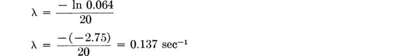
and mean
![]()
Thus the probability paper can be used conveniently both to judge the validity of the proposed type of distribution and to estimate the particular parameters that seem to fit the data best. Unless a systematic method† is used to fit the line, however, it is not possible to determine the statistical properties of parameter estimates found in this way.
Normal probability paper Normal probability paper and its graphical construction from the CDF are illustrated in Fig. 4.4.8. So that the bar-yield data can be compared to a normal model (Fig. 4.4.9) a convenient horizontal scale is determined and the values of i/(n + 1) are plotted versus xi. As with the exponential case, comparison of the data with a normal model can be made independently of specific parameter values by asking if the data points fall (within reasonable sampling variation) upon a straight line. In this case a positive answer again seems justified. Comparison with a specific normal model, say N (8490,1032), is possible once the straight line corresponding to these parameters is plotted (see Fig. 4.4.9). As before, one can also fit by any reasonable
Fig. 4.4.8 Construction of normal probability paper, (a) Linear scale; (b) probability paper.
Fig. 4.4.9 Bar-yield-force data on normal probability paper.
method (by eye in the case of the dashed line shown) a straight line to the data and use it to estimate the parameters. Given such a line, the corresponding mean is found at the abscissa x of the line’s intersection with FX(x) = 0.50, and the abscissa x of FX(x) = 0.841 is approximately the mean plus 1 standard deviation. The dashed line, then, corresponds to the normal distribution with m = 8495 lb and
![]()
In general, changing the mean shifts the straight line laterally, while increasing the standard deviation flattens it. Thus both the location and scale parameters of the distribution can be estimated by the paper.
Fig. 4.4.10 Five truncated normal distributions on normal probability paper. (Adapted from Hald [1952].)
Fig. 4.4.11 The exponential distribution on normal probability paper.
Fig. 4.4.12 Three log-normal distributions on normal probability paper. (Adapted from Hald [1952].)
Different models on the same paper It is important to be able to recognize how the CDF of one distribution appears on the probability paper of another. A number of these cases are shown in Figs. 4.4.10 to 4.4.15.
Notice (Figs. 4.4.10 and 4.4.11) that distributions with abruptly
Fig. 4.4.13 Five binomial distributions on normal probability paper.
Fig. 4.4.14 First asymptotic extreme-value probability paper. (Adapted from Gumbel[1958].)
falling PDF’s (e.g., exponential or truncated normal), lead to sharply falling (or rising) curves on normal paper (depending on which tail of the curve the fall occurs in). The effects of skew are also observable. Notice that a normal distribution fit in the region of the mean would overestimate F(x) in the upper tails of positively skewed distributions (e.g., Fig. 4.4.12). The CDF of a discrete random variable shows jumps at certain values (Fig. 4.4.13).
Other probability papers have also been constructed and found useful. Figure 4.4.14 is extreme-value paper for the Type I asymptotic distribution. Lognormal probability paper is most easily obtained by simply transforming the horizontal, numerical scale of normal paper to a logarithmic one. Figure 4.4.15 shows several normal distributions plotted on lognormal paper of this kind. By a similar transformation
Fig. 4.4.15 Lognormal probability paper.
(Sec. 3.3.3) Type II and Type III asymptotic extreme-value papers can be constructed from Type I paper (if the parameters ω or ![]() of the Type III distribution are known). The papers do not provide estimates for these third parameters of three parameter distributions.
of the Type III distribution are known). The papers do not provide estimates for these third parameters of three parameter distributions.
Discussion In order to interpret properly the qualification that the model is acceptable if the data points fall “within reasonable sampling variation” about a straight line, we should study the cumulative frequency polygon as a (complicated, vector-valued) sample statistic. Various approaches are possible,† but it is sufficient for our immediate purposes to state that, by analogy with the histogram, the conclusions of such a study would be:
1. The cumulative frequency polygon is a sample statistic, exhibiting random variation about the true CDF.
2. Perfect agreement between the observed cumulative frequency polygon and the model CDF may be the single most likely outcome, but it is a very unlikely event.
3. If another model is in fact controlling the observations, the observed cumulative frequency polygon may or may not seem to support (incorrectly) the engineer’s hypothesized model. The likelihood that it will depends on how nearly similar in shape the true law is to the hypothesized one.
In Sec. 4.4.2 a simpler statistic will be introduced which will permit quantification of many of these conclusions. In addition, plots on probability paper in that section (Figs. 4.4.16 and 4.4.17) will demonstrate graphically another most important fact. When compared on probability paper, wide excursions of the cumulative frequency polygon are very likely to occur in regions of distributions where the paper’s scale causes major distortions. These include the upper tail of an exponential distribution and both tails of a normal distribution. Such excursions appear in the data plotted in Figs. 4.4.7 and 4.4.9. The important implication is that what seem to be large discrepancies between the last few data points in these tails and the straight-line fit through points in the central portion of the data can seldom be interpreted as a sufficient reason to reject the proposed model. Such occurrences are simply not unlikely, even if the model holds.
In this section we shall combine some of those ideas in the previous section about the nature of observed shapes of data with the technique of the hypothesis test developed in Sec. 4.2. In this case the null hypothesis will be the model proposed by the engineer. Thus one might encounter such a hypothesis as
![]()
or
![]()
or, lacking a specific parameter value,
![]()
The alternate hypothesis, namely, that the variable is not as H0 claims, is grossly composite. For example, if X is not N(100,152) it might be N(110,152) or N(100,202) or N(120,122) or it might not even be normally distributed at all, but rather lognormal or gamma or any of an infinite variety of named and unnamed continuous, discrete, or mixed distributions. While the computation of the type I error probability will turn out to be possible, it is clear that β, the type II error probability, is a function of not only other parameter values, but also other distribution types, and it is hardly amenable to complete description.
We shall consider two different hypothesis tests with similar forms, forms that differ only in the specific test statistic. We require some sample statistic D, which, roughly speaking, measures the deviation of the observed data shape from the model predicted shape. Such a statistic might, for example, be related to the differences between the histogram proportions Ni/n and the predicted fraction 1/k, discussed in Sec. 4.4.1. The form of the operating rule is:

If we know that under H0, the statistic D has some particular distribution, we can calculate the value of c associated with any desired significance level α. In principle we might also be able to compute the value of β for any particular alternate model, but clearly there is no end to such alternate distributions and no meaningful way to summarize such results.
Having computed c, one would observe the underlying random variable n times, find the value of D, compare this with c, and report the conclusion to accept or reject the proposed model.
Observe that the purpose of the test is solely to answer the question of whether the data deviate a statistically significant amount from the model prediction.
χ2 Test The first such hypothesis test we shall consider is by far the more popular, having been proposed by an early statistician, Karl Pearson, in 1900. It is called the χ2 goodness-of-fit test. The statistic used is related to the histogram’s deviations from the predicted values. Suppose we have a model for a discrete random variable X. If we (randomly) sample that random variable n times, the number Ni of observations of the ith possible value xi of X is a random variable with the binomial distribution, since the probability of observing the ith possible value in each test is constant, with value pi = P[X = xi] = px(xi). The expected value of Ni is npi, and its variance is npi(l – pi) (see Sec. 3.1.2). If npi is not too small, the standardized random deviation from the expected value
is approximately N(0,l), as shown in Sec. 3.3.1. It should not be unexpected then that D'1, the sum of the squares of these standardized deviations
has approximately the χ2 distribution (Sec. 3.4.3). The sum might be over the k possible values of the random variable X if each npi is sufficiently large that the approximation is valid. If not, we shall resort to lumping, which will be demonstrated shortly.
Owing to the lack of independence among the Ni (notice that a linear functional relationship  exists), the number of degrees of freedom of the χ2 variable is not k but k – 1 and each term is decreased by a factor (1 – pi). These corrections can be hueristically justified by noting that if the square of one deviation is larger than average owing to the chance occurrence of an “extra” observation at that value, then the square of some other deviation (that associated with the value which was “shorted”) is also necessarily larger than average. More formal derivations are available in Hald [1952] and Cramer [1946]. Finally, then, the statistic
is approximately χ2-distributed with k – 1 degrees of freedom. From tables of this distribution we can determine critical values ![]() for any value of k – 1 such that
for any value of k – 1 such that
After observing a sample of the random variable X, we can compute the observed value of the D1 statistic and compare it to the value ![]()
Illustration: Discrete random variable with specified parameter Consider, for example, the rainstorm data reported in Table 4.4.1. Under the null hypothesis that rainstorms occur at these (independent) stations with an average rate of occurrence of one per year and that the occurrences are Poisson arrivals Sec. 3.2), the distribution of the number of arrivals X each year at any station is Poisson-distributed with mean (and parameter) 1.
![]()
If the model holds, the expected numbers of observations of each value of x in a sample of size 360 are as shown in column 1 of Table 4.4.1. Subtracting each expected value from its observed value, squaring, and dividing by the expected number yields the normalized squared deviations (column 2, Table 4.4.1). Notice that the last two categories have been lumped together to give a single category with a larger expected number of observations. This is done to insure that the approximation of the statistic’s distribution by the χ2 distribution is adequate. A conservative value for the smallest expected number of observations permissible in any category is 5 to 10 (Cramer [1946] and Hald [1952]), but more recent experiments† have shown that tests based on expected values as low as two or even one give satisfactory results (Lindley [1965], part II, page 167; Fisz [1963], page 439).
The observed statistic is d1 = 16.68. Under the null hypothesis, the distribution of D1 is approximately χ2 with 5 degrees of freedom, since there are, after lumping, k = 6 categories considered here. The probability of such a χ2 random variable exceeding 16.68 is less than 0.005. ‡ In particular, for a significance level of α – 5 percent, the critical value is
![]()
Since d1 = ![]() , hypothesis should be rejected at the 5 percent level. In words, the engineer should report that there is a significant difference between the shape of the data and the model, a Poisson distribution with parameter 1.0 storms per year.
, hypothesis should be rejected at the 5 percent level. In words, the engineer should report that there is a significant difference between the shape of the data and the model, a Poisson distribution with parameter 1.0 storms per year.
χ2 Test: estimated parameters It is rarely the case that the engineer’s experience is sufficient to suggest a hypothesis which includes a value of the distribution’s parameter. Normally he hypothesizes the form of the distribution, but estimates the parameter or parameters from the data itself. Is it reasonable to use this same data to help judge the goodness of fit of the model? It is if we account for the fact that the data have also been used to estimate the model parameters. The more parameters a distribution has, the closer it can be fit to given data. We account for this effect by simply reducing the number of degrees of freedom of the distribution of the statistic by one for each parameter estimated from the data (Hald [1952], Cramer [1946]). This reduction of the degrees of freedom has the effect of reducing the value c which the statistic must be less than in order that the null hypothesis be accepted. In other
Table 4.4.1 The annual number of rainstorms recorded at a number of stations
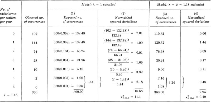
Source: E. L. Grant [1938].
words, because we have used the same data to partially fit the model to the data, the statistic must be smaller to be acceptable at the same significance level. It can be said that in such cases we are testing the proposal that the distribution is of a particular type or shape, parameter values being unspecified (at least until after the observations).
Formally, the number of degrees of freedom of the statistic D1 is
where k is the number of categories considered and r is the number of parameters estimated from the data. Clearly if r = k – 1, there could be perfect agreement between observed and expected numbers. This occurs, for example, if one attempts to apply a goodness-of-fit test to a sample of a zero or one Bernoulli (k = 2) random variable whose single (r = 1) parameter p has been estimated by the ratio of the number of successes to the number of trials. Recall, by analogy, that we can always fit a polynomial of degree k – 1 through any k points.
Illustration: Discrete random variable, estimated parameter It is more likely, for example, that the engineer studying rainstorms would have hypothesized simply a Poisson model, only later adopting a parameter (mean) equal to the estimate provided by the observed sample mean, ![]() = 1.18 storms per year. With this parameter the expected number of observations are given in column 3 and the normalized squared deviations in column 4 of Table 4.4.1. The observed statistic is now d1 = 2.95, suggesting a considerably better fit between model and data. In this case we must compare, however, with a χ2 random variable with 6 – 1 – 1=4 degrees of freedom. The critical value at the 5 percent level of significance is
= 1.18 storms per year. With this parameter the expected number of observations are given in column 3 and the normalized squared deviations in column 4 of Table 4.4.1. The observed statistic is now d1 = 2.95, suggesting a considerably better fit between model and data. In this case we must compare, however, with a χ2 random variable with 6 – 1 – 1=4 degrees of freedom. The critical value at the 5 percent level of significance is ![]() . Since 2.95 ≤ 9.49, this hypothesized model is not to be rejected. Given that the model holds, the probability (the p level) was about 60 percent that a value of D1 as large as or larger than 2.95 would be observed.
. Since 2.95 ≤ 9.49, this hypothesized model is not to be rejected. Given that the model holds, the probability (the p level) was about 60 percent that a value of D1 as large as or larger than 2.95 would be observed.
χ 2 Test: Continuous random variables The χ2 goodness-of-fit test can also be applied to continuous random variables. It is only necessary to divide the region of definition of the variable into a finite number of intervals and compute (through integration over each of the intervals) the probability pi of the random variable’s being in each of the intervals. Such intervals are often chosen in much the same manner as those for histograms (Chap. 1.1). In fact, as discussed in Sec. 4.4.1, what is being compared by the test is the degree of fit between an observed histogram and a density function lumped into a corresponding bar-form PDF or discrete mass function.
If we consider, as an example, the yield-force data and the intervals used in the histogram in Fig. 4.4.1, we are led to Table 4.4.2. The expected number of occurrences in an interval is computed by multiplying the sample size times the probability of the random variable’s
Table 4.4.2 Histogram intervals for bar-yield-force model and data
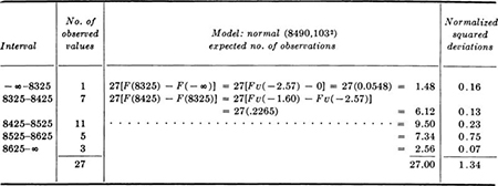
taking a value in the interval; this probability is determined as the difference between the values of the cumulative distribution function at each end of the interval. The hypothesized model is normal with the parameters estimated from the data: ![]() = 8490;
= 8490; ![]() = 103. Hence the number of degrees of freedom of the statistic D1 is 5 – 2 – 1 = 2. At the 5 percent significance level the critical value is
= 103. Hence the number of degrees of freedom of the statistic D1 is 5 – 2 – 1 = 2. At the 5 percent significance level the critical value is ![]() = 5.99, a value much greater than the observed value of 1.34. (The probability that a χ2 random variable with 2 degrees of freedom will exceed 1.34 is about 50 percent.) This data are not in significant contradiction to the model.
= 5.99, a value much greater than the observed value of 1.34. (The probability that a χ2 random variable with 2 degrees of freedom will exceed 1.34 is about 50 percent.) This data are not in significant contradiction to the model.
It is desirable, † particularly when dealing with continuous random variables, to seek intervals width equal pi (as in Sec. 4.2.1). Once a number of categories k has been decided upon, the interval division points can be determined from a table as those values of x where, for the hypothesized model, F(x) = 0, 1/k, 2/k, etc. Notice that this approach removes the arbitrary process of interval selection associated with histograms. ‡
That the choice of intervals may be important can be observed in Table 4.4.3, where 10 intervals were used for the yield-force data, giving an expected number of observations of 2.7 in each category. This number is somewhat smaller than the commonly recommended smallest expected number, 5. The observed value of D1 is d1 = 17.07, and the appropriate number of degrees of freedom is 10 – 2 – 1 = 7, yielding ![]() . Since
. Since ![]() the test suggests that the model be rejected at the 5 percent level of significance, a decision counter to that arrived at previously. The hypothesis would, however, be accepted at the 1 percent level, where
the test suggests that the model be rejected at the 5 percent level of significance, a decision counter to that arrived at previously. The hypothesis would, however, be accepted at the 1 percent level, where ![]() . The reader may wish to show that if a test based on five intervals each of probability 20 percent and expected number of observations 5.4 is adopted, the hypothesis would be
. The reader may wish to show that if a test based on five intervals each of probability 20 percent and expected number of observations 5.4 is adopted, the hypothesis would be
Table 4.4.3† Uniform probability intervals for bar-yield-force model and data
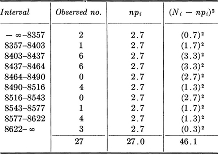

rejected at both of these levels of significance. It is not clear how the engineer should react when two tests on the same data lead to contradictory conclusions. What is important is to realize that the popular χ2 test is open to such contradictions. This limitation should be kept in mind when reviewing the reported results of χ2 tests.
Kolmogorov–Smirnov test A second quantitative goodness-of-fit test is based on a second test statistic. It concentrates on the deviations between the hypothesized cumulative distribution function FX(x) and the observed cumulative histogram†
in which X(i) is the ith. largest observed value in the random sample of size n. Consider the statistic
In words, D2 is the largest of the absolute values of the n differences between the hypothesized CDF and the observed cumulative histogram (sometimes called the empirical CDF) evaluated at the observed values
in the sample. It has been found (Massey [1951], Birnbaum [1952], Fisz [1963]) that the distribution of this sample statistic is independent of the hypothesized distribution of X. Its only parameter is n, the sample size. Knowing this statistics distribution, we can compute the critical value c and perform an hypotheses test at a prescribed significance level. Such a test is called the Kolmogorov–Smirnov goodness-of-fit test.
As before

The form of the operating rule is
![]()
The test statistic is now D2, given in Eq. (4.4.18).
The determination of d2, the observed value of the statistic, is facilitated if a graphical comparison of the cumulative histogram and the CDF of the hypothesized model is available. In the case of the bar-yield-force example the plot on probability paper, Fig. 4.4.9, can be searched quickly to find likely locations of the near maxima of ![]() . [Notice that if probability paper plotting points i/n rather than i/(n + 1) had been used, the points on this figure would define exactly rather than approximately the cumulative histogram F*(x(i)), Eq. (4.4.17)]. See the footnote on page 468. By inspection, possible locations for the maximum include x(12) = 8440, x(15) = 8460, and x(18) = 8500. For these values
. [Notice that if probability paper plotting points i/n rather than i/(n + 1) had been used, the points on this figure would define exactly rather than approximately the cumulative histogram F*(x(i)), Eq. (4.4.17)]. See the footnote on page 468. By inspection, possible locations for the maximum include x(12) = 8440, x(15) = 8460, and x(18) = 8500. For these values
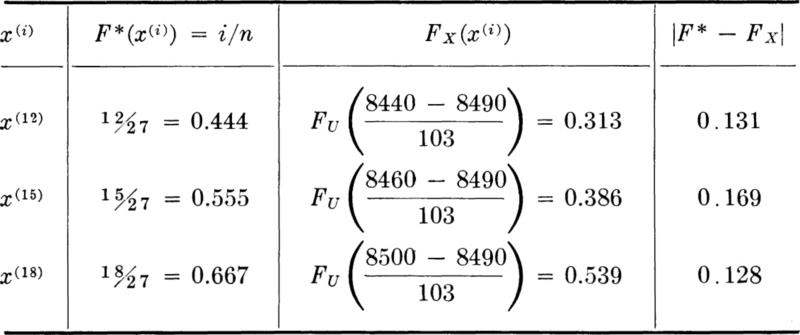
Consequently, d2 = 0.169. The critical value for n = 27 and α = 0.05 is, from Table A.7, about 0.256. Since d2 is less than the critical value, we conclude that the model should not be rejected. (Recall, incidentally, that two of three χ2 tests led to the model’s rejection.)
Discussion of Kolmogorov-Smirnov test The Kolmogorov-Smirnov test has an advantage over the χ2 test in that it does not lump data and compare discrete categories, but rather compares all the data in an unaltered form. The value of the statistic D2 is also usually computed more easily than D1 especially if the data has been plotted on probability paper. Unlike the χ2 test, the Kolmogorov-Smirnov test is an exact test for all sample sizes. On the other hand, the Kolmogorov-Smirnov goodness-of-fit test is strictly valid only for continuous distributions and only when the model is hypothesized wholly independently of the data. Nevertheless, the test is often used† for discrete distribution tests, when it is conservative, and for the case in which parameters have been estimated from the same data, when it is not known quantitatively how to adjust the distribution in a manner analogous to subtracting degrees of freedom in the χ2 test. If the parameters have been estimated from the data, it can be said only that the critical value should be reduced in magnitude.
Graphical execution of Kolmogorov-Smirnov test It is also possible to carry out quantitative goodness-of-fit evaluations in a graphical manner. It is worthwhile to consider this topic if for no other reason than its ability to help us visualize the effects of statistical uncertainty on the distribution as a whole. This graphical technique can best be carried out directly on probability paper as we shall do here.
Notice first that the Kolmogorov-Smirnov test just discussed can be conducted by plotting curved lines above and below the hypothesized CDF offset by an amount equal to the critical value determined from the table of the distribution of the statistic D2. In the bar-yield-force example just considered this value was 0.256. In Fig. 4.4.16, the hypothesized distribution N (8490,1032) is plotted, along with curves offset by an amount 0.256. That none of the observed plotting points falls outside this line implies that the hypothesized model should not be rejected at the 5 percent significance level. ‡ Curves for the 20 percent significance level (with critical value 0.20) are also shown in order to indicate the effect of the level of significance. At this level also the hypothesized model should not be rejected. The tighter curves indicate a larger likelihood of rejecting the model when it is correct, but there is less chance that the model will not be rejected when another model holds (type II error).
The most striking feature of the curves representing the acceptance
Fig. 4.4.16 Bar-yield-force data and model: Kolmogorov-Smirnov test.
region is their wide flare in the tails of the distribution. This is a graphical representation of the uncertainty surrounding tail areas of distributions, owing to the small likelihood associated with values of the random variable in these regions. Very large deviations of the larger and smaller values of the sample must occur before they can be considered “practically impossible” (i.e., significantly unlikely, < 5 percent, say) to have occurred given this model.
It should be stated again that with this Kolmogorov-Smirnov test no correction is available to account for the fact that the hypothesized model parameters were estimated from the data itself. Such a correction would take the form of tighter curves about the hypothesized line.
Illustration: Traffic-gap data Let us conduct the quantitative goodness-of-fit tests on the traffic-gap data presented in Table 4.1.2 and plotted in Fig. 4.4.2. The hypothesized model (based recall, on the assumption that the traffic is Poisson) is that a gap time is an exponential random variable. The parameter λ has been estimated from the data to be 0.130 sec-1.
To perform a χ2 goodness-of-fit test we shall first consider using 20 categories of equal expected number of observations, (1/20) (214) = 10.7. The corresponding interval divisions can be determined sufficiently accurately by using the solid straight line in Fig. 4.4.7, which corresponds to the hypothesized model. These intervals are indicated in Table 4.4.4. Owing to the rounding off to the nearest second which occurred in the reporting of the data, several of the first intervals do not contain abscissas (even half-seconds) at which plotting took place. One might consider lumping the first 10 categories to form 5 each containing a plotting abscissa and each with expected number (2/20) (214) = 21.4, as shown in Table 4.4.4. Such lumping, first of the observed data and then of the categories for the χ2 test, is undesirable in regions of large expected numbers, since it introduces artificial errors in the numbers actually observed in each interval used in the test. If the reported data have been lumped (owing, for instance, to lack of measuring instrument sensitivity or, as here, to ease reporting), it is preferable to pick goodness-of-fit test intervals to coincide with reporting intervals and to determine (nonequal)
Table 4.4.4 Goodness-of-fit test: equal-probability intervals for traffic-gap-data illustrations
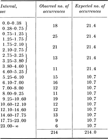
Table 4.4.5 Goodness-of-fit test for traffic-gap-data illustration
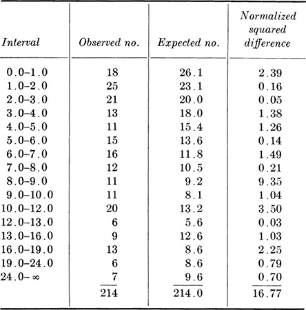
expected numbers for each. Such 1-sec intervals and their corresponding expected numbers are shown in Table 4.4.5. When the expected number dropped below 10, eight intervals with expected values averaging approximately 10 were determined, still with boundaries coinciding with those used in reporting. The observed value of the test statistic is found to be 16.77. The statistic has 16 – 1 – 1 = 14 degrees of freedom. The critical value at the 5 percent level of significance is 23.7 (Table A.2), implying that the model should not be rejected at this level.
The Kolmogorov-Smirnov test is carried out graphically in Fig. 4.4.17. The critical value at the 5 percent significance level is ![]() (Table A.7). Lines of this value either side of the hypothesized model are drawn as shown. The model should not be rejected, since all points lie within the band. The modifications to the plotting points associated with using i/n in place of i/(n + 1) clearly would not affect this decision.
(Table A.7). Lines of this value either side of the hypothesized model are drawn as shown. The model should not be rejected, since all points lie within the band. The modifications to the plotting points associated with using i/n in place of i/(n + 1) clearly would not affect this decision.
Illustration: Highway-construction quality-control data Existence of a physical model of the underlying mechanism may not be the reason that an engineer proposes a particular distribution for a variable. Computational convenience or other professional circumstances may suggest that a particular model be used if possible.
A first step in setting up statistical quality-control methods in the highway-construction field has been the determination of the distributions of the commonly measured and controlled variables, such as embankment compaction, asphalt content, depth of subbase, aggregate gradation indices, etc. Statistical
Fig. 4.4.17 Traffic-gap data: Kolmogorov-Smirnov test.
methods of quality control are best developed and simplest to use if the underlying variable is normally distributed. Successful field implementation requires simple and uniform procedures.
Suppose that the normal distribution has been judged to be a satisfactory representation of the other variables of interest and, now, based on data, a decision must be made about whether “percent relative compaction” can also be treated as a normally distributed random variable when the new methods are introduced. To be forced to reject the hypothesis that this variable was normal would require setting up a special procedure for it (tables different from those used for the other variables, etc.), which would make the whole new program less palatable and possibly delay its acceptance by the industry. Consequently, the engineer seems justified in adopting a very small significance level, say α = 1 percent, when conducting a goodness-of-fit test on this data.
The data are given in Table 4.4.6 and, as a histogram, in Fig. 4.4.18 (Beaton [1967]). Should the null hypothesis that this variable is normally distributed be accepted at the 1 percent significance level?
Table 4.4.6 Kolmogorov-Smirnov test for illustration involving percent relative compaction data
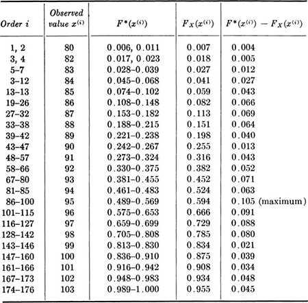
Source: Beaton [1967].
The parameter estimates are:

Fig. 4.4.18 Percent relative compaction of roadway embankment.
The values of F*(x(i)) = i/n and FX(x{i)) are tabulated in the same table. The largest discrepancy is:
![]()
For an α level of 1 percent and a sample size of 176, the critical value of the Kolmogorov-Smirnov statistic is ![]() (Table A.7). Therefore, the hypothesis need not be rejected at this significance level. The variable may be treated as if it were normally distributed.
(Table A.7). Therefore, the hypothesis need not be rejected at this significance level. The variable may be treated as if it were normally distributed.
It is important to realize that had the engineer, for other reasons, set up a null hypothesis that this variable was gamma-distributed or lognormally distributed or any one of many other choices, the conclusion might very well have been the same: that he could accept that hypothesis. It cannot be emphasized too strongly that the goodness-of-fit test is not designed to discriminate among two or more distributions or to help the engineer choose from among several contending distributions. Rather its purpose is to help answer the question, “Can I use the distribution toward which I have a certain predisposition or is the data in such apparent discord with this model that I must reject it?”
Discussion Two general comments on goodness-of-fit tests are in order before closing this section. The first is on the one-sided form of the rule, “Accept H0 if D ≤ c.” Recall from the previous section that perfect fits (D = 0) are very unlikely. Also, since many different observed histograms will lead to the same (nonzero) value of D, it is no longer even true that D = 0 is necessarily the most likely outcome. Consider the χ2 statistic. It has a gammalike distribution (Sec. 3.4.3) with a mean equal to the number of degrees of freedom, k – r – 1. For k – r – 1 greater than 1, the mode, or most likely† value, of D is k – r – 3. For larger numbers of degrees of freedom at least, very small values of D are as unlikely as very large. There have been proposals, in fact, that two-sided goodness-of-fit tests be used, although it is not clear what alternate hypothesis is considered consistent with very small values of D. Certainly alternative distributions can only tend to yield large values of D since for these models E[Ni – npi] does not equal zero (pi being based on the null hypothesis).
Secondly, goodness-of-fit hypothesis tests should be open to the same critical review given any hypothesis tests (Sec. 4.2). The selection of the significance level remains solely a matter of convention. The balancing of type I error versus type II error probabilities, which should be carried out in principle, becomes impossible in light of the form of the alternative hypothesis. As mentioned, it contains not only the same model with other parameter values, but also an infinite variety of other forms of
distributions. In addition the goodness-of-fit tests have certain limitations of their own, as discussed above (dependence on interval choice, for example). Nonetheless, if the reader of a report which includes a goodness-of-fit test to substantiate the model choice uses proper judgment in its interpretation, there is value and convenience in the conventional application of these tests.
A proposed model can be verified only by comparing its predictions with observed data. In the case of probability distribution models, the comparison is usually between the shape of the distribution (PDF or CDF) and the shape of the data (histogram or cumulative histogram).
The usual comparison is made difficult by the fact that the data “shape” is a sample statistic subject to random fluctuations. In the case of histograms the comparison is further complicated by the dependence of the variability of this statistic on the number of intervals used. This number also dictates the degree of resolution or lack of resolution (“smearing”) associated with the bar-form PDF vis-à-vis the complete PDF.
Analytical hypothesis tests are also available to compare data and model. The χ2 goodness-of-fit test is based on a statistic

which measures the discrepancy between histogram and bar-form PDF. The Kolmogorov-Smirnov test uses the deviations between the observed cumulative histogram and the CDF.
In the previous section we dealt with the situation in which a particular distribution had been suggested and the validity of that assumption was in question. In other situations the problem may be one of selecting a distribution from among a number of contending mathematical forms when no single one is preferred on the basis of the physical characteristics of the phenomena. The situation may also arise when any convenient, “reasonable” distribution is adequate for the purposes at hand. The engineer may simply be looking for a tractable, smooth mathematical function to summarize the available data because subsequent dealings with the variable will be simplified by this representation.
The treatment of such selection problems will be considered briefly in this section. These selections are often strongly influenced by professional considerations, so generalizations are difficult. Statistical theory offers little quantitative help. Our format here, therefore, will be to present illustrative examples and to raise our major points within the context of these problems. A brief summary of these points will then suffice for guidance in other situations.