WWW To download the web content for this chapter go to the website www.routledge.com/cw/wright, select this book then click on Chapter 4.
Regardless of the method used to pull a matte, there are a variety of operations that can be applied to refine its quality. In this chapter several techniques are described that remove noise, soften edges, expand or contract the matte size, and sculpt the edges to get a better composite.
Before we begin refining mattes there is a very important technique that I would like to share with all of you keyers out there. As we saw in the last two chapters every matte you pull, including with the keyers, invariably has to be scaled up in the whites and down in the blacks to achieve 100% white in the target region and zero black in the backing region. The key to these scaling operations is to go just far enough to clear out the problem areas – but no further – because if you over-scale the matte the edges become harder and the fine hair detail disappears. The technique I call “gamma slamming” is a huge help with this very delicate balance.
The idea behind gamma slamming is that by “slamming” the gamma down hard it reveals the transparencies and thin spots in the core of the matte, then slamming the gamma up hard in turn reveals noise or contamination in the backing region. This amounts to a brightness “magnifying glass” that allows you to peer deeper into the matte to see defects and dial them out. You can use this to advantage to avoid over-scaling your mattes because this technique shows you exactly when you have reached the perfect point.
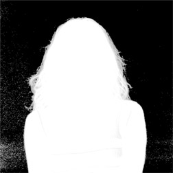
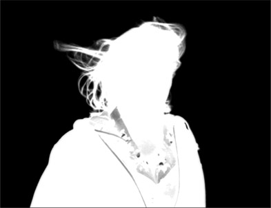
Starting with Figure 4.1 we have a supposedly “clean” matte with no visible defects. If we apply a gamma correction of around 0.1 to the matte it “pulls down” hard on the whites exaggerating even small deviations from exactly 1.0, revealing any thin spots, transparencies, or “grain holes” in the matte as shown in Figure 4.2. You then very gently increase the scaling up of the whites just enough to make these defects disappear – and no more. This exaggerated view makes it easy to know exactly when to stop. And knowing when to stop is essential to avoid over-scaling the matte.
Next, the gamma is dialed way up to around 3.0, which now stretches the blacks and reveals any noise or contamination in the backing region like Figure 4.3. The blacks can now be scaled down – very tenderly – just until the noise is just gone, and no more. To be honest, it is not necessary to completely clear out every single particle of contamination in the backing region. Leaving a slight residual will not be noticed in the final comp and may allow you to retain a bit more fine edge detail like hair, which is always a good thing.
Many compositing programs have a gamma adjustment for the viewer where you view images so you can adjust the gamma of the viewer contents but not change the data in the original image. This makes it very quick and easy to view the image with different gamma settings. If your software does not have this feature an easy work around is to add a gamma operation to your matte downstream of where you are scaling it. You can then connect your viewer to the gamma operation while you adjust the black and white scaling upstream. When everything looks good just delete or disable the gamma operation to return the matte to normal.
 TIP! When scaling mattes be sure to never let the code values go below zero or above 1.0 as that can introduce unpredictable behavior in your composites. This can be tricky when working in float because the regular RGB images can go negative or super-white (above 1.0), but mattes must always be clamped to stay between zero and one.
One of the first preprocessing operations to be done for virtually any greenscreen keying process is to garbage matte the backing color. The basic idea is to replace the backing area all the way out to the edges of the frame with a clean, uniform color so that when the matte is extracted the backing region will be clean and solid all the way out to the edges of the frame. There are two important criteria to this operation. First, that it replaces the greenscreen a safe distance away from the edges of the target object. You must make sure that it is the keying process that creates the target object’s edges, not the garbage matte. The second criteria is that it does not take too much time to create.
There are basically two ways to generate the garbage matte – procedurally (using rules), and manually (rotoscope). Obviously, the procedural approach is preferred because it will take less time. A chroma key or even another keyer can be used to pull a rough key, then dilated to pull it away from the edges of the target object. Failing that you can always draw a roto, but that will be more time consuming. Because we are trying not to get too close to the edges of the foreground object the rotos can be loosely drawn and the keyframes spaced far apart depending on the action in the shot. The two methods can also be combined by pulling a matte for most of the backing region plus a single garbage matte for the far outer edges of the screen, which may be badly lit or have no greenscreen at all.
A garbage matte can be applied to the original greenscreen prior to keying to provide a clear and solid backing region out of the keyer. Figure 4.4 shows the original green-screen plate with an uneven backing color getting darker towards the corners of the frame. Figure 4.5 is the garbage matte to be used, and Figure 4.6 is the resulting garbage matted greenscreen. The backing region is now filled with a nice uniform green all prepped for a nice key. Note that the garbage matte has been softened around the edges a bit to avoid a sharp edge that may show up in the key. Notice also that the garbage matte did not come too close to the edges of the foreground. Also, most keyers have some way of presenting garbage mattes to it that will be used internally for its calculation of the key. Read the manual.
However you end up creating it, simply composite the foreground object over a solid plate of green. But what green to use? The RGB values of the backing differ everywhere across its surface. As you can see in the garbage-matted greenscreen of Figure 4.6 the color of the filled area is darker than the remaining greenscreen in some areas and lighter in others. You should sample the actual greenscreen RGB values near the most visually important parts of the greenscreen, typically around the face if there is a person in the shot. This way the best matte edges will end up in the most visually important part of the picture.
Garbage mattes can also be applied after the key is pulled. Again, these can be hand drawn roto mattes, procedural mattes, or a mix. Figure 4.7 shows the original key with problems in both the backing region and the core area of the key. Instead of being a nice clean black all around the backing region has some contamination due to poor uniformity in the original greenscreen. The key’s core also has some thin, low density areas that will result in some transparency in the target. This we must fix.
Figure 4.8 is a garbage matte created procedurally by using a simple chroma key on the backing region. The chroma key was made with tight settings so that only the green-screen is keyed. It was also dilated (expanding the white areas) to pull it away from the original matte so that it does not touch any of its edges and accidentally trim them away. Figure 4.9 shows the results of clearing the backing region with its garbage matte. One way to do this is to multiply the original key by the backing garbage matte so the garbage matte’s black pixels zero out the original key’s backing region. A second approach is to use the garbage matte as a mask for a color correction operation on the original key to clear the backing region.

Figure 4.11 Core of key cleared
With the backing region well under control in Figure 4.9 we can turn our attention to cleaning up the thin areas in the core of the key. The “core” refers to the 100% solid white area of the matte and excludes the semi-transparent edges. Figure 4.10 shows a core garbage matte that was made from the original key. The first step is to increase the contrast of the original key so there are no thin spots in the core or contamination in the backing region. The second step is to perform an erode operation to shrink the garbage matte enough that it fits everywhere inside the original key. Again, our garbage mattes must not touch the edges of the key.
Once the core matte is prepared it can be used to clear the main key with a Maximum operation (see Chapter 13: Image Blending). The Maximum operation will compare the core matte with the main key on a pixel-by-pixel basis selecting whichever pixel is the brightest. When a pixel in the main key is less then 100% white the Maximum operation will output the pixel from the core matte so the final key will everywhere be 100% white in its core. After all the garbage matting is completed a careful inspection should be done to double check that they nowhere touch the edges of the main key. An easy way to do that is to toggle the garbage mattes on and off frame-by-frame to see if the main key’s edges move. The key’s edges must be created only by the keyer, never a garbage matte.
In this section we will explore filtering a matte with a blur or Median filter. There are three reasons why you might want to filter a matte. First, to remove noise. Second, to soften the edges. And third, to do your own dilate or erode operation.
Regardless of what matte extraction technique is used – a keyer for a greenscreen or rolling your own luma key – there may be some residual noise in the matte even if the original plate has been degrained. By eliminating this noise prior to scaling the matte we will not have to scale it so hard, which results in nicer matte edges and the retention of more edge detail. Here we will see why this is so.
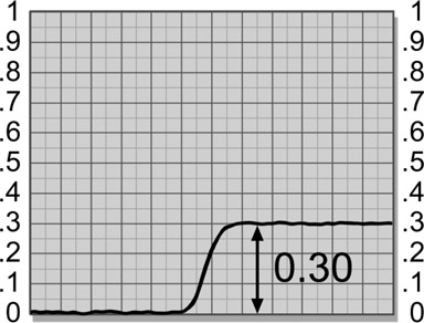
Figure 4.12 is a slice graph of a noisy (grainy) raw matte. The noise causes the pixel values to “chatter” both up and down. This tends to close the useable gap between the foreground region (around 0.3) and the backing region (near 0), to a useable gap of only about 0.2. This 0.2 region is all that is available for the final scaled matte if you are trying to eliminate the noise by scaling alone.
Figure 4.13 shows the effects of a filtering operation. It has smoothed out the noise in both the backing and foreground regions. As a result, the gap has opened up to 0.3, increasing the available raw matte density range by 50%. (All numbers have been exaggerated for demo purposes so your results may vary). However, if you pull a matte on a nicely shot greenscreen with a minimum amount of noise you may not have to perform this operation on the raw matte, so feel free to skip it when possible.
The filtering operation to use for removing noise is the Median filter, not a blur. The Median filter is much more selective at going after small details like noise and minimizes the amount of fine detail damage. Allow me to illustrate.
Figure 4.14 shows a close-up of the original matte with lots of fine hair detail. When the gamma is slammed down to 0.1 in Figure 4.15 it reveals lots of “grain holes” in the matte. We wish to remove the noise with the least damage to the edges and fine hair detail.
Figure 4.16 shows the results of a very small Median filter size of just 1 pixel, which was enough to remove all of the noise. Note how the hair detail still compares very favorably with the original matte in Figure 4.14. Next we try a blur size of 6 in Figure 4.17, which actually did not totally clear out all of the noise but did do major damage to the fine hair detail. So, to lose the noise and keep the fine detail use a small radius Median filter.
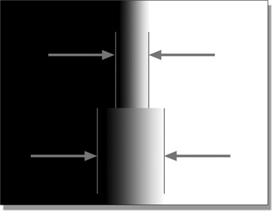
When softer edges are needed the blur operation is performed on the final matte after it has been scaled to full density. The blur softens the composited edge transition in two ways. First, it mellows out any sharp transitions, and second it widens the edge, which is normally good. It is important to understand what is going on, however, so that when it does introduce problems you will know what to do about them.
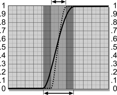
Figure 4.18 shows a slice graph of a matte’s edge transition between the white and black regions. The dotted line represents the matte before a blur operation, with the short arrow at the top of the graph marking the width of the edge transition. The steep slope of the dotted line indicates that it is a hard edge. The solid black line represents the matte after a blur operation, and the longer arrow at the bottom marks the new width of the edge transition. The slope of the solid line is shallower, indicating a softer edge. In addition to the softer edge it is also a wider edge.
The blur operation has taken some of the gray pixels of the transition region and mixed them with the black pixels from the backing region, pulling them up from black. Similarly, the white pixels of the foreground region have been mixed with the gray transition pixels, pulling them down. As a result, the edge has spread both inward and outward equally, shrinking the core of the matte while expanding its edges.
This edge-spreading effect can be seen very clearly in Figure 4.19. The top half is the original edge, and the bottom half is the blurred edge. The “borders” of the edge have been marked in each version, and the much wider edge after the blur is very apparent. This edge expansion often helps the final composite, but occasionally it hurts it. You need to be able to increase or decrease the amount of blur and shift the edge in and out as necessary for the final composite – and all of this with great precision and control. Not surprisingly, the next section is about such precision and control.
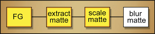
Figure 4.20 Blur applied to scaled matte to soften edges
Figure 4.20 shows a flow-graph with the blur operation added after the matte-scaling operation for softening the edges of the final matte.
A blur operation has two parameters to set for the best results – the blur radius and the blur percentage. The blur radius affects how “aggressive” the blur is, and the blur percentage controls the mix-back with the original plate.
A blur operation works by replacing each pixel in the image with an average of the pixels in its immediate vicinity. The first question is, what is the immediate vicinity? This is what the blur radius parameter is about. The larger the radius, the larger the “immediate vicinity”. To take a clear example, a blur of a radius of 3 will reach out 3 pixels all around the current pixel, average all those pixel values together, then put the results into the current pixel’s location. A blur of radius 10 will reach out 10 pixels in all directions, and so on.
So what is the effect of changing the radius of the blur? The larger the blur radius, the larger the details that will get hammered (smoothed). By the way, signal engineers do not refer to the details getting “hammered”. They prefer to say they were “filtered out”.

Figure 4.21
Smoothing effects of increasing the blur radius
Figure 4.21 shows a slice of a noisy image with the results of various blur radiuses. Each version has been shifted down the graph for readability. The top line represents the original noise. The middle line shows the results of a small radius blur that smoothed out the tallest small “spikes”, but left some local variation remaining. With a larger blur radius the lower line would result in the local variation smoothed out and just a large overall variation left. Of course, increasing the filtering like this also increases the loss of edge detail.
More sophisticated blur operations will also allow you to choose the type of filter algorithm to use for the blur. You might have choices such as Gaussian, box, or triangle. Each one will deliver a slightly different result so try each one to see which works best for your particular situation.
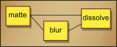
The second blur parameter, which I am calling the blur percentage, is actually a “mix-back” percentage. It goes like this: take an image and make a blurred copy. You now have two images, the original and the blurred. Next, do a cross-dissolve between the blurred image and the original image, say a 50% dissolve. You are mixing back the original image 50% with the blurred image, hence a “mix-back” percentage. That’s all there is to it. And now, if your package does not offer a “percentage” parameter (by this or some other name) you now know how to make your own. Use a dissolve operation to create your own “percentage” parameter as shown in Figure 4.22. It will add an additional node, but gives you an extra control knob over the strength of the blur, and control is the name of the game in compositing visual effects.
If you do not have a dissolve operation, then scale the RGB values of the unblurred version by (say) 30% and the blurred version by 70%, then sum them together with an add node to make 100%. Changing the ratios (so they always total 100%, of course) allows any range of blur percentage.
Another aspect of controlling a blur operation is masking it off from areas that you don’t want blurred – such as hair, for example. Use one of the many mask-generating techniques in Chapter 2: Pulling Keys, to generate a mask that either isolates the area that you want to blur or masks off the areas that you don’t want blurred.
Sometimes the finished matte is “too large” around the perimeter, revealing dark edges around the finished composite. The fix here is to shrink or “choke in” on the matte by moving the edges in towards the center. Most software packages have dilate (expand) and erode (shrink) ops that operate on the white part of the matte. Use them if you’ve got them, but keep in mind that these edge-processing ops destroy edge detail too. These edge-processing ops “walk” around the matte edge adding or subtracting pixels to dilate or erode the perimeter. While these operations usually retain the soft edge (falloff) characteristics of the matte, keep in mind that the fine edge details such as hair will still get lost. Figure 4.23 illustrates the progressive loss of edge detail with increasing matte erosion. Note especially the loss of the fine hair detail.

Figure 4.23
Progressive loss of edge detail as the matte is eroded
Virtually all compositing programs have dilate and erode edge-processing operations so you might be wondering why you should know how to erode a matte yourself with blur and scale operations. The reason is control. Many dilate and erode operations only move in single pixel jumps and that can create a problem. One setting is too large, the next too small. The work around is to “roll your own” dilate or erode with this blur-and-scale technique that is exquisitely adjustable. The following techniques show how to convert the gray edge pixels into either black transparency or white opacity regions, thus dilating or eroding the matte.
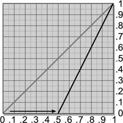
Figure 4.24 represents a finished matte that needs some refinement. The edge has been made very soft in order to make the process more visible. Figure 4.25 shows how to adjust the color lookup curve to erode (shrink) the blurred matte shown in Figure 4.24, with the results in Figure 4.26. By pulling “down” on the blacks, the gray pixels that were part of the edge have become black and are now part of the black transparency region. By moving the color lookup only slightly, very fine control over the matte edge can be achieved. The foreground region has shrunk, tucking the matte in all the way around the edges, but the edges have also become harder. If the harder edges are a problem, then go back to the original blur operation and increase it a bit. This will widen the edge transition region a bit more giving you more room to shrink the matte and still leave some softness in the edge at the expense of some lost of edge detail. Note the loss of detail in Figure 4.26 after the erode operation. The inner corners (crotches) are more rounded than the original, an artifact called “filleting”. This is why the minimum amount of this operation is applied to achieve the desired results.
To see the difference between using an edge processing operation or the color lookup tool to erode the matte, Figure 4.27 shows a slice graph of the edge of a soft matte that has been shifted by an edge-processing operation. Note how the edge has moved inwards but has retained its slope, which indicates that the softness of the original edge was retained. Compared to Figure 4.28, the same edge was scaled with a color lookup as described above. While the matte did shrink, it also increased its slope and therefore its hardness increased. Normally, only small changes are required so the increase in edge hardness is usually not a problem. However, if an edge-processing operation is available and offers the necessary fine control it is the best tool for the job.
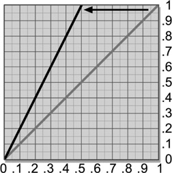
Figure 4.30 shows how to adjust the color lookup curve to expand the blurred matte in Figure 4.29 (the same matte as in Figure 4.24), with the results shown in Figure 4.31. By pulling “up” on the whites, the gray pixels that were part of the inner edge have become white and are now part of the foreground white opacity region. The opaque region has expanded, and the edges have become harder. Again, if the harder edges are a problem, go back and increase the blur a bit. And yet again, watch for the loss of detail. Note how the star points are now more rounded from filleting than the original.
The above operations were described as eroding and dilating the matte, while in fact they were actually eroding and dilating the whites, which happened to be the foreground matte color in this case. If you are dealing with black mattes instead, such as when pulling your own color difference mattes, then the color lookup operations would simply be reversed or the matte inverted.
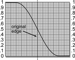
When a blur is applied to a matte both the 100% white core and the zero black regions shift away from the original edge. The vertical dashed line in Figure 4.32 represents the original edge of a hard matte and the curved line represents the new edge falloff after a blur with a lovely “S” curve. Note that the core has move to the left, away from its original position at the dotted line, which results in shrinking the core of the matte. But sometimes you don’t want to shrink the core.
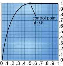
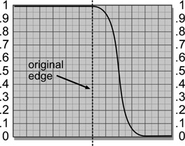
The solution is to do a “blur out” operation such that the edges of the matte are blurred outward only without shrinking the core of the matte. How this is done is illustrated in Figure 4.33 where a color lookup is applied after the blur to reshape the falloff of the edge of the matte to preserve the original core size but still providing the soft outer edge of the blur operation. Note the control point at 0.5 on the color lookup and that the right side of the curve is perfectly horizontal. A control point at this location brings the blurred edge from 50% gray to 100% white, which restores the original core edge. However, if the color lookup is simply a straight line the falloff will exhibit a sharp edge at the inner edge of the core. By applying a curve as shown in Figure 4.33 the inner edge gets a nice “shoulder” and the falloff at the foot of the curve is preserved. Figure 4.34 illustrates the new falloff of the matte edge preserving the original core size but retaining the soft outer edge.
You can add another layer of control over your edges (and we love control!) by literally sculpting the edge falloff of the alpha channel of the key with a color lookup curve. You have pulled your finest key, but when the premultiplied foreground is composited over the background the edges of the comp are less than gorgeous. Not a problem. Following the flowgraph in Figure 4.35, the premultiplied foreground is first unpremultiplied (very important!), then the alpha channel is sculpted with a color lookup curve, the RGB layer is re-multiplied with a premult operation, then the lovely new results are comped over the background.
This workflow cannot be done, of course, if you are compositing inside the keyer as it must be done prior to the comp over the background, which would place this operation inside the keyer. Not to worry, we will see how to do the composite outside the keyer in Chapter 6: The Composite.
Figure 4.38
Edge sculpted 2
We can see the profound effect of this technique starting with the original edge in Figure 4.36. The falloff from the inner core edge is a bit stark and unnatural-looking. Figure 4.37 shows the edge sculpted for a much more natural-looking falloff using edge sculpting curve 1 in Figure 4.39. Or we could tuck the edge in using the color lookup curve in Figure 4.40. The key points are to perform the unpremult first, apply the color lookup to the alpha channel only, then re-multiply the results. This ensures that the RGB values along the edge stay in balance with the alpha channel and do not grow darker or lighter than they should.
One thing I should mention is that this operation on the alpha channel will affect all semi-transparent alpha pixels. If there are semi-transparent elements in the comp or other edge regions that you do not want to affect then they will have to be masked off to protect them. Keep in mind that if you are having edge troubles with a keyed element the Add-Mix node (again, see Chapter 6: The Composite) also gives great edge control.
As long as we are talking about edges, it occasionally comes to pass that you would like a mask of only the edges of a key. One way to do that, of course, is to use an edge detect tool. However, sometimes the edge detection tool does not give you enough control, so here is another way to “roll your own” edge mask with exquisite control.
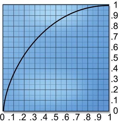
The basic idea is illustrated in Figure 4.41. On the left is the original key, in the middle is a color curve that is applied to the key, and on the right is the resulting edge mask. The edges of a key are a gradient ranging from 1.0 in the core to zero at the edge. The color curve has a control point at 0,0 which leaves the blacks untouched. The middle control point is set for 0.5, 1.0 which brings the middle gray pixels in the edge up to solid white. The last control point at 1.0, 0 takes the whites in the core down to black. The result is a mask made from just the edge pixels – plus any semi-transparent pixels within the key, of course.
If the initial edge mask is too thin for your purposes then run a small blur on the key to throw more pixels into the edge gradient. Another adjustment is to widen the top of the curve, which will thicken the core of the edge matte but not affected its width. Moving either of the end control points in towards the center will thin the edge mask with the left control point moving the black edge and the right control point moving the white edge.
WWW Keying Frames – this folder contains the same four keying challenges from Chapter 3 for you to try the matte refinement techniques outlined above.
So far we have seen how to create novel keys, how to work with keyers, and now methods of refining our keys for the best edges possible. In the next chapter we will take on the obscure topic of spill suppression, or despill. This is a terribly important subject because spill turns up in the target object, the edges, motion blur, and any depth-of-field areas. We will learn what causes spill and how to defeat it, in order to create our finest composites.