So far we have focused on keying and the despill operation, all of which was to set us up for this chapter – The Composite. This chapter is all about the many different ways that the foreground and background images can be combined into the final composited image. And why do we need so many ways to do things? Because of my lament in Chapter 3: Working with Keyers, where I declared keying to be an elaborate cheat that often does not work very well.
This chapter starts off with the story of premultiply and unpremultiply, because it is central to the compositing process and many are unclear about it. More importantly, getting it wrong can give you discolored edges in your comps. We have to lock that down before we move on. We then jump right into it to see the workflow for all the steps of a composite then look over several types of operations for performing the composite such as the Over, the KeyMix and the AddMix operations, plus the truly awesome Processed Foreground Method. Don’t miss that one!
We will also explore several workflows for doing the composite inside a keyer and the pitfalls therein, followed by multiple strategies for compositing outside the keyer. This chapter then finishes up by exploring stereo compositing, the stereo conversion process, and a myriad of tips for working in the wonderful world of stereo compositing. Sounds like a lot of material to cover, so we should get started right away.
Before starting the exciting subject of the composite I want to clear up a persistent confusion to many visual effects artists, namely what is premultiply and unpremultiply. It is based on multiplying the RGB channels by the alpha channel and it appears everywhere in the subject of compositing. The basic idea is that the pixels of the RGB layer are rendered at full color and all of the transparency information is in the alpha channel for anti-aliased edges, motion blur, and semi-transparent elements. The RGB layer is then multiplied by the alpha channel to darken those RGB pixels that are over semi-transparent alpha channel pixels. But why is it called “premultiplied”?
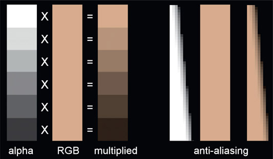
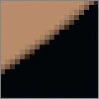
Referring to Figure 6.1 the left strip represents an alpha channel with various values from 100% white (1.0) to nearly black as a series of grey chips. If the RGB strip next to it is multiplied by the alpha strip the resulting multiplied image will be scaled down by the value of its alpha chip. So, for example, an alpha chip with a code value of 0.5 will scale the RGB code values down by 0.5 so it will get darker. The resulting multiplied strip now gets progressively darker from top to bottom. The anti-aliasing example to the right illustrates this multiply operation in action to introduce anti-aliasing to the solid strip in the center. Of course, alpha channel values of less than 1.0 are also used to introduce semi-transparency to RGB images overall, not just anti-aliased edges.
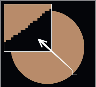
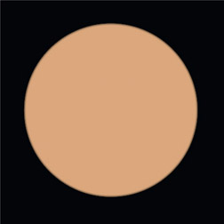
So how does the multiplying of two images together apply to the term “premultiply”? The answer lies in the history of CG. In the very early days of CG the images were rendered in two separate passes – the raw RGB pass which contained the full color of each pixel, and the transparency pass which held the transparency information for each pixel. An example of such a raw RGB pass is shown in Figure 6.2. Note in the inset close-up that it has the jaggies – there is no anti-aliasing yet.
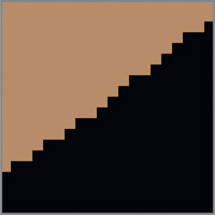
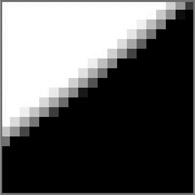
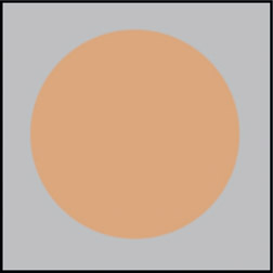
The early compositor would receive these two passes and the first thing he did was to multiply the raw RGB pass shown in Figure 6.3 by the transparency pass shown in Figure 6.4 to introduce the anti-aliasing shown in Figure 6.5. As CG rendering technology advanced the transparency pass was added to the RGB pass in a 4th channel which they named “A” for “alpha”, but the compositor still had to multiply the raw RGB layer by the alpha channel. The next improvement was for the CG rendering software to perform the multiply of the raw RGB by the alpha channel in order to introduce anti-aliasing to the edges of the CG. Since the CG renders now came to the compositor already multiplied they referred to it as a premultiplied image. We have been stuck with this term ever since.
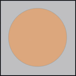
There are many situations in visual effects where we need to undo the premultiplication in order to restore the original RGB values of the anti-aliased or semi-transparent pixels. Since the premultiply was done by multiplying the raw RGB by the alpha channel, it can be reversed by dividing the premultiplied image by its alpha channel – which is the unpremultiply operation (Figure 6.6). As you can see, the unpremultiplied image in Figure 6.6 now looks exactly like the original raw RGB pass in Figure 6.3.
Greenscreen keying also produces a premultiplied image which at times needs to be unpremultiplied, so this is no longer just a CG thing. Note that this unpremultiply operation must be done with great mathematical precision (many decimal places) to avoid round-off errors, which is yet another reason the industry has gone “float”.
There are two cardinal rules that you must always follow when working with premultiplied images:
Cardinal Rule #1 – color correction and color space conversions must be performed on the unpremultiplied image (like Figure 6.6). Bet you didn’t see that one coming.
Cardinal Rule #2 – transformations (rotate, scale, etc.) and filtering operations (blur, etc.) must be performed on the premultiplied image (like Figure 6.5).
Why these rules exist is explained and demonstrated in their respective chapters on color correction and animation for transformations. For now, commit them to memory and make sure that you always follow them to avoid getting into color trouble in your composites. Now, though, you know the true story of premultiply vs. unpremultiply.
A common mistake in compositing premultiplied images is to accidentally give it a second premultiply, and if that happens the edges will go dark. What you don’t want to do is go in there and try to fix the dark edges with some kind of an edge treatment. That just introduces compensating errors. The right answer is to go upstream of the dark-edge comp to find and then remove the double premultiply.
We can follow the double premultiply action starting with the premultiplied image in Figure 6.7. When composited over a nice background like Figure 6.8 the edges look fine. However, if a second premultiply were done to the original premultiplied image in Figure 6.7 you may not notice it until it is actually comped over the background, like in Figure 6.9, where the telltale dark edges have suddenly shown up.
The reason the edges go dark is because the first premultiply scaled the edge pixel RGB values darker, based on the transparency of the alpha channel. At this point the darkened edge pixels are “in balance” with the semi-transparent pixels of the alpha channel. For example, if a semi-transparent alpha pixel was 0.5 then its RGB pixel will be scaled by 0.5, making it darker by half. But when it is composited it will be mixed with a background pixel also scaled by 0.5 so that everything balances out (Figure 6.8). However, a second premult operation would scale that same RGB pixel by 0.5 twice, or (0.5 × 0.5 =) 0.25, so now the RGB values are twice as dark as before – hence the dark edge (Figure 6.9).
WWW Premult_RGB.tif & premult_transparency.tif – the year is 1962 and you have been given an unpremultiplied RGB layer with a separate transparency mask. Your mission is to move the transparency mask into the alpha channel of the RGB image and perform the premultiply operation prior to compositing it over a background. Also try an unpremultiply to restore the RGB layer back to the original image.
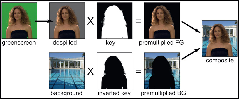
Now that we have the premultiply/unpremultiply issue sorted out we can take a look at the fundamentals of a composite illustrated in Figure 6.10. Starting with the greenscreen in the upper left corner, it is despilled then multiplied by the key. This clears the despilled backing region to zero black producing the premultiplied foreground. Moving to the second row and starting with the background, it is multiplied by the same key (inverted), which produces the premultiplied background. Summing the premultiplied foreground and premultiplied background together produces the finished composite.
These are the sequence of operations that all keyers use to produce a composite and they are the very steps needed when compositing outside the keyer which we will look at later in this chapter. There are also compositing tools that take care of some of this work for you, which we will look at next.
The Over composite illustrated in Figure 6.11 was originally developed for compositing 4-channel RGBA CG renders (the CG render is shown here along with its alpha channel for clarity). It assumes the CG render is a 4-channel premultiplied image and performs the actual composite over the background. All the Over operation has to do is premultiply the background layer and sum it with the premultiplied foreground.
While intended for compositing CG it is also frequently used for greenscreen compositing outside the keyer. However, you have to prepare the greenscreen layer as a 4-channel premultiplied RGBA image because that is what the Over operation is expecting.
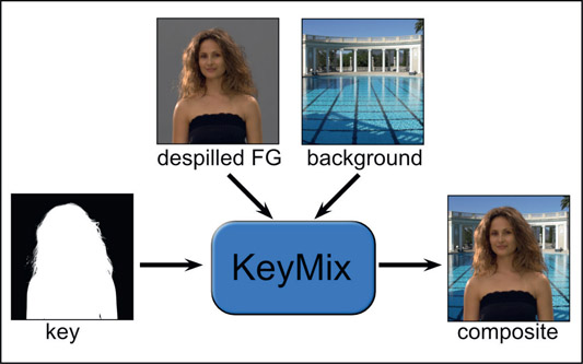
The KeyMix composite is yet another way to combine the foreground and background into a composite. Referring to the illustration in Figure 6.12, the KeyMix operation has three inputs – the despilled foreground, background and the key are separately connected to the KeyMix node. Inside the KeyMix, the despilled foreground will be premultiplied by the key, the back ground will be premultiplied by the inverted key, then the results summed together to produce the output composite.
This is visually and mathematically identical to the composite workflow in Figure 6.10. It’s just that all of the math operations are being performed for you inside the KeyMix node. This is one alternative workflow when compositing outside the keyer that allows you access to the key and despilled foreground which you don’t have when compositing inside the keyer. You could, for example, dilate and soften the key or color correct the despilled foreground upstream of the KeyMix node. When compositing inside the keyer the only control you have is what the keyer designers decided to give you.
The AddMix composite is a variation on the normal compositing algorithm that can be especially helpful when compositing thin wispy elements such as dust or smoke, light emitters such as laser beams, as well as to clear up those pesky dark edges around someone else’s composite – after you have made sure there is no double-premultiply lurking in the comp. The AddMix compositing operation is identical in all regards to the normal composite except when it comes to scaling the foreground and background by the matte. With the normal composite the same matte is used to scale the foreground layer, then inverted before scaling the background layer. With the AddMix composite, color lookup curves are used to make two different versions of the matte – one for the foreground and one for the background layers.
So how does the AddMix composite work and when should you use it? How it works is a bit difficult to visualize. The color lookup curves do not affect the matte in either the 100% transparent or 100% opaque regions. It only affects the partial transparency pixels of the matte, which means it affects the composite in two areas – the semi-transparent regions and the anti-aliased pixels around the edge of the matte. The effect of that is to alter the relative mixing of the foreground and background semi-transparent pixels based on how the color curves are adjusted.

Figure 6.13
Effect of AddMix color lookup curves on edges
If you have an AddMix tool you will be presented with two color lookup curves – one for the foreground (FG) and one for the background (BG). If you don’t have an AddMix tool see Section 6.2.3.2: How to Build It for complete instructions on how to roll your own. Referring to the first case: on the left of Figure 6.13 (Over composite) the two curves are unaltered so the results will be an ordinary Over composite. If the curves are adjusted upward the edges will get lighter (AddMix lighter), and curved downward the edges get darker (AddMix darker).
Each curve is affecting the brightness of its own edges independently. You could, for example, increase the brightness of the foreground (FG) curve but darken the brightness of the background (BG) curve. The effect would be to increase the “presence” of the foreground color and reduce the presence of the background color – though only at the edges, of course, plus any other semi-transparent regions.

Figure 6.14
Flowgraph of the AddMix compositing operation
To create the AddMix composite, color lookup nodes are added to the key just before it performs the multiply on the foreground and background, as shown in Figure 6.14. The key here is that the matte edges can be adjusted differently for the foreground and background. That is the whole point. With the conventional compositing operation a color curve could be added to the matte before the scaling operations, but it is the same matte used for scaling both the foreground and background. Here, the matte is different for the foreground and the background scaling operations.
Some compositing systems do have an AddMix compositing operation, and if yours does then you are doubly blessed. If not, then you can use the flowgraph in Figure 6.14 to “roll your own”.
One of the occasions to use an AddMix composite is when compositing a wispy element such as dust, smoke or thin fog. Figure 6.15 shows a smoke element that was self-matted then composited over a night city. The smoke is barely seen. In Figure 6.16 an AddMix composite was used to thin the matte on the smoke element but not the city element to give the smoke layer more presence. Again, this is an entirely different result than you would get just by tweaking the matte density in a normal composite.

Figure 6.15 Normal composite of a smoke plate over a night city

Figure 6.16
AddMix composite causes the smoke layer to have more presence
Another occasion where the AddMix method can be helpful is when compositing “light emitters” such as laser beams, fire or explosions. The example in Figure 6.17 shows an example of another dastardly laser attack by the demonic planet Mungo on our precious Rocky Mountain resources. Whether the beam element was rendered by the CGI department or keyed out of another plate, the AddMix composite can be used to adjust the edge attributes to give the element a more interesting and colorful appearance like Figure 6.18. Notice that the edges have not lost their transparency or hardened up in any way.

Figure 6.17
Standard composite of beam element over a background

Figure 6.18
The AddMix composite adds energy to the beam
A more prosaic application of the AddMix method is cleaning up those pesky dark edges often found lurking around a composite. While there are many causes and cures for them that will be covered in later sections, one of those cures can be the AddMix composite. Figure 6.19 shows a close-up of a dark edge between the foreground and background while Figure 6.20 shows how the AddMix composite can clean things up nicely. Again, make sure that the dark edges are not from a double-premultiply.
WWW Composite Kit – this folder contains the images from Figure 6.12 for you to try the Over, KeyMix and AddMix compositing techniques above.
So far we have seen the classical method of compositing – multiply the despilled foreground plate by the matte, multiply the background plate by the inverted matte, then sum the results together. But there is another way – a completely different way – that can give better results under many circumstances: the processed foreground method. Its main virtue is that it produces much nicer edges, retaining more hair detail under most circumstances compared to the classic premultiplied foreground method. I suspect that this is the secret sauce in the Keylight keyer that allows it to retain so much fine hair detail.
The secret of the processed foreground method is in how it clears the backing region to black. In a regular composite the despilled foreground would be multiplied by the key (or premultiplied if you prefer) to clear the backing region to black. This multiply operation also scales down the fine hair detail. The processed foreground method avoids this by not multiplying the foreground by the key. Instead, the key multiplies a solid plate of the despill color. That is then subtracted from the despilled foreground to clear the backing region. The fine hair detail remains at full brightness.
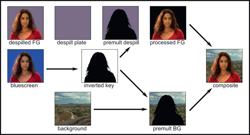
Figure 6.21 illustrates the step-by-step workflow for doing a processed foreground composite. Try it. You’ll like it.
Step 1 – starting with the bluescreen on the left, pull your best key and invert it.
Step 2 – prepare the despilled foreground (upper left corner) using your best spill suppression technique.
Step 3 – prepare the despill plate which is just a solid plate of the despilled backing color in the despilled foreground (step 2).
Step 4 – prepare the premultiplied despill plate by multiplying the inverted key (step 1) by the despill plate (step 3).
Step 5 – prepare the processed foreground by subtracting the premultiplied despill plate (step 4) from the despilled foreground (step 2). Critical note – follow this subtraction with a clamp to avoid negative numbers.
Step 6 – prepare the premultiplied background by multiplying the background plate by the inverted key (step 1).
Step 7 – make the composite by summing the processed foreground (step 5) with the premultiplied background (step 6).
So how much difference does the processed foreground method make? Compare the processed foreground composite in Figure 6.22 to the standard premultiplied Over composite in Figure 6.23. On the left side of the head you can see far more light hair strands than with the premultiplied comp. On the right side of the head the dark hair strands are more dense and defined. These two examples were made with the exact same despilled foreground and key. The only difference was the math used to combine them in a comp.
The processed foreground method can produce some wonderful edge detail, especially hair. However, it can also have a couple issues that you should watch out for. When the processed foreground plate is created there will be residual grain in the black surround that will end up being added to the background at the last step. Hopefully this will be minor, but if not, degrain just the black surround by using the alpha channel as a mask. Do not degrain the entire plate because the grain on the character must be preserved – unless your workflow removes all the grain at the beginning then restores all the grain after the composite.
Uneven lighting in the greenscreen/bluescreen backing region can end up contaminating the final composite. Underlit regions are not a problem because they are darker and do not show up in the black backing region, but hot spots will leave a residual backing region of the processed foreground which will then be added to the background during the final composite at step 7. If this happens then sample the despilled backing region in its hottest spot to make the despill plate.
Yet another solution is to make a clean plate from the despilled foreground from step 2 using the “blur and grow” technique from Chapter 2: Pulling Keys. The best fix, however, is to have a perfectly uniform backing region by using the screen correction technique covered in Chapter 3: Working With Keyers.
WWW Processed Foreground – this folder contains a bluescreen and the BG from Figure 6.21 for you to try the processed foreground method. Compare it to a standard premultiplied comp and prepare to be amazed.
All compositing programs come with one or more keyers and the sales brochure says that all you have to do to get a perfect composite is connect the greenscreen here and the background there, then make a few adjustments. Done. Then you tried it with your own clips and experienced nothing but misery. This is the way of keying. It is such a large problem because color space is huge and an infinite amount of mischief can reside in your greenscreen plates.
The cruel truth is that you will rarely get a great comp by using a single keyer. One keyer does not fit all greenscreens and bluescreens, no matter what the sales brochure says. I teach my students that in the real world you will invariably have to use what I call the “divide and conquer” strategy – divide the problem into separate pieces that you can conquer one at a time. This means using more than one keyer. Following are some strategies for using multiple keyers, with the keyers doing the actual composite – well, at least their piece of it.
It seems that there are always two conflicting keying requirements. On the one hand you want lots of fine hair detail in the edges, but you also want 100% density in the key. In many cases these are mutually exclusive requirements. You can pull a matte that has lots of great detail around the edges, but the matte has insufficient density to be completely solid. When you harden up the key to get the density you need, the edges harden and the fine details disappear. The soft comp/hard comp procedure provides a useful solution for this problem, and best of all, it is one of the few procedures that does not introduce any new artifacts that you will have to go pound down. It’s real clean.
The basic idea is to do two composites, one on top of the other. The first composite is with a “soft” key that has all of the edge detail but lacks full density so it produces a semi-transparent composite over the background. The second composite is laid down on top of the first, but with the keyer adjusted for a harder key that is fully opaque. The process of dialing in the harder key will also pull its edges in so that the hard comp actually fits inside the soft comp. It is essential that the soft comp provides the outer edge detail leaving the hard comp to provide the inner solid core.

Figure 6.24
Soft comp/hard comp sequence of operations
This workflow requires the use of two (or more) keyers. You can use the same brand keyer (e.g. Keylight) with different settings for both the hard and soft comps, or use two different keyers (e.g. Keylight and Primatte). Here are the steps for the soft comp/hard comp procedure:
Step 1 – create the “soft” key. It has great edge detail, but does not have full density in the core.
Step 2 – do the soft comp. Composite the foreground over the background with the soft matte. A partially transparent composite is expected at this stage.
Step 3 – create the “hard” key from the bluescreen with a second keyer. It has to be totally opaque and fit inside the soft comp edges.
Step 4 – do the hard comp. Comp the foreground with the hard key over the first comp using it as the background. The hard key fills in the solid core of the foreground, and the soft comp handles the edge detail.
The soft comp/hard comp method above is rather like stacking keyers on top of each other. This approach is rather like laying them side-by-side like two interlocking pieces of a jigsaw puzzle, each covering a different area. This strategy is to use two or more keyer setups – each optimized for a different part of the picture – then cut and paste the good parts together. Say, for example, that one keyer setup does a great job on the hair, but not the shirt. Another keyer setup does a fine job on the shirt, but not the hair. So we want to cut and paste the good hair key with the good shirt key. This is one approach to a fine composite, as long as you avoid the pitfalls and problems.
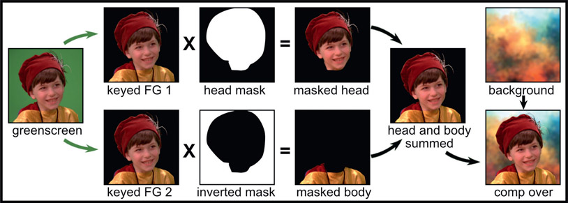
In the workflow example in Figure 6.25 we will be optimizing two keyers, one for the head and one the body, then combining them into a single hero comp. You can use two of the same brand keyer (e.g. Keylight) with two different settings, or use two different keyers (e.g. Keylight and Primatte).
Step 1 – set up two keyers to output despilled and premultiplied foregrounds, one dialed in for the head and the other for the body (keyed FG1 and keyed FG 2).
Step 2 – create an isolation mask for the head (head mask) and multiply it by the keyed FG1 to produce the masked head.
Step 3 – invert the head mask (inverted mask) and multiply it by the keyed FG2 to produce the masked body.
Step 4 – sum the masked head and masked body together (head and body summed).
Step 5 – use an Over operation to composite the summed head and body over the background.
And now for the pitfalls and problems. Do not make the mistake of first compositing the masked body over the background then compositing the masked head over that. Although it may sound like a reasonable thing to do, upon close inspection you will find a visible seam between the two parts. The other thing to watch out for is, since you are using two different keyers, the despill may not be identical between them – even if you use the same type keyer for both keys (e.g. two Keylight keyers). Even with the identical keyer the different settings within the keyer may alter the spill suppression results. Not good. Adding a wide soft edge to the seam between the two pieces may blend any despill differences gently enough to avoid being noticed. Still, if you follow the rules, and don’t have a spill suppression difference, this approach can quickly give good results.
WWW Cut and Paste – this folder contains the greenscreen and BG from Figure 6.25 for you to try the workflow outlined above.
Compositing outside the keyer is the way the big kids work simply because it gives you the most control – and control is the name of the game in visual effects. The downside is that it is more complicated and you have to actually know what you are doing. Too bad there isn’t a really great book on keying to learn from! Oh well. We’ll muddle through somehow.
The whole idea here is to take your life in your own hands, pull your best key (you can use a keyer for that), do your best despill, use your key to premultiply the greenscreen and background plates, then comp them together yourself – all outside of the keyer. We will see a variety of approaches here because, as I said up front, keying is a cheat that works fairly well most of the time, so we will need lots of fallback positions to survive.
The workflows from here on get a bit more complex so I am switching to using node graphs from Nuke to help tell the story. But all of these techniques are carefully written to be useable in any software, even a layer-based compositor like After Effects. By following these procedures you will add several powerful new techniques to your skillset that will put some real hair on your mouse.
Things get a bit more complex here, so it seems like a propitious moment to raise an important principle for all compositors, and that is always to avoid interdependencies in your comps. For example, if you did a resize operation on a plate then followed that with some roto work. That would be bad because the roto depends on the resize and any change to that will blow up your rotos. So roto on the base resolution plate, then resize it for the comp. Avoiding interdependencies like this is one of the background thought processes that we compositors must always carry out to avoid self-inflicted wounds that require unnecessary repair work.
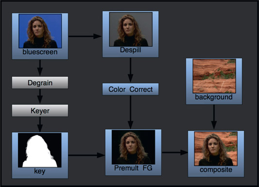
As an opening gambit we will start with the overall keying and compositing workflow outside the keyer where a single key was able to do the job (chuckle). A compositing node graph of the single key is shown in Figure 6.26, which represents the simplest case showing the entire workflow. Starting with the bluescreen in the upper left hand corner and proceeding down, the first step is the obligatory degrain operation to remove noise. Any other pre-processing to sweeten the bluescreen for the keyer would go here too. Next, using your favorite keyer, pull your best key. We are only going to use the key – nothing else produced by the keyer.
Starting back at the top with the original bluescreen (not the degrained version), to the right is your favorite despill operation, then after that is the color correction for the foreground. The despill and color correction must always be done in that order. If you did color correction first, then later when you revised it (and you will always revise the color correction) the despill settings will blow up and have to be completely redone. So despill first, color correction second. Always.
If you are going to use an “over” operation then the foreground must be a 4-channel premultiplied image. There are few ways to get there from here. First, copy the key into the foreground’s alpha channel and from there you could perform a normal premultiply operation. If, for some odd reason, you don’t have an official premultiply operation then you could substitute a Gain down to zero operation that is masked by the alpha channel. The results would be mathematically identical. Should you be contemplating the KeyMix operation you would leave the despilled foreground, background and key separate, as it requires each on a separate input. If going for an AddMix, you may or may not need to prepare a premultiplied foreground, depending on the whims of the designer of your AddMix node.
This workflow represents just a basic outline of the process of keying outside the keyer. The next refinement would be to massage the key to refine the edges, apply a garbage matte, and other beautifications to the key that we learned about in Chapter 4: Refining Mattes.
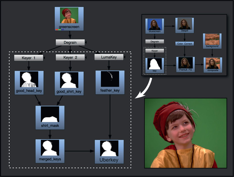
Figure 6.27
Merging multiple keys to create an “Uberkey”
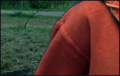
The previous example demonstrated the workflow for compositing outside the keyer with a single key. Here we will build on this concept by creating the “Uberkey”, a master key that combines the best parts of several flawed keys – the most common workflow for experienced visual effects compositors. Figure 6.27 shows a close-up of the green-screen with feathers in the hat, which are hard to key. The inset in the upper right corner shows the area from the single key workflow in Figure 6.26 that we are expanding on. To get a good key for this greenscreen we needed to pull two keys plus a luma key, then combine all three into the Uberkey. The techniques for creating and combining keys were covered in Chapter 4: Refining Mattes. Here we will see how they fit into the overall workflow of compositing outside the keyer.
Keyer 1 pulled a good key for the head but the shirt was too thin. Keyer 2 pulled a good key for the shirt but the feathers were chewed up. The good head key and good shirt keys are masked by the shirt mask and combined to produce the merged keys. Neither keyer had good results for the hat feathers so a separate luma key was pulled for the feathers and combined with the merged keys to produce the finished Uberkey for compositing. The point here is that the Uberkey is created by any number of keying techniques, not just keyers. We can combine luma keys, chroma keys, color difference keys – anything it takes to get a great key for each part of the foreground object.
WWW Uberkey – this folder contains the greenscreen from Figure 6.27 plus a BG for you to try your hand at an Uberkey. Pay particular attention to capturing all of the feather detail in the hat.
In Section 6.3: Compositing With a Keyer, above, we were compositing inside the keyer and saw how to combine the 4-channel premultiplied outputs of the keyers into a final composite. Here we will see the same workflow for compositing outside the keyer. The big difference being that here we are only working with the keys produced by the keyers, not their 4-channel premultiplied foreground outputs.
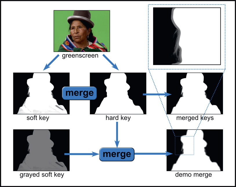
The soft key/hard key workflow is illustrated in Figure 6.28. A soft key is pulled that retains all the fine hair detail but does not have a solid core. We don’t care about the core here. What we really want is all that fine hair detail. A hard key is pulled that is solid as a rock but no hair detail. It must also be eroded to fit everywhere inside the soft key because the objective is for the soft key to define the edges and the hard key to fill in the core without touching those edges.
These two keys are merged together with either a Maximum or a Screen operation, never summed. Summing them will result in code values above 1.0, which must never be done for keys or mattes. The Maximum and Screen operations will give slightly different results where the mattes overlap, which is addressed in exquisite detail in Chapter 13: Image Blending.
The grayed soft key is just a darkened version of the original soft key for demo purposes here, in order to make the edges visible in the demo merge. The gray edges protrude all around the perimeter of the hard key because the hard key is everywhere inside the perimeter of the soft key. This is critical because the hard key must never touch the edges. The edges must always be defined by the soft key.
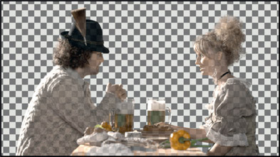
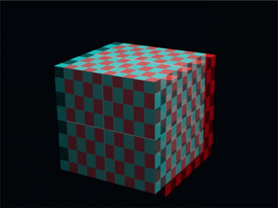
The additive keyer is grievously misnamed. It’s not really a keyer. It is a sophisticated mathematical melding of the foreground and background images like a sophisticated Photoshop blend operation that appears rather like a semi-transparent composite – but there is no key. As a result, there is no loss of fine edge detail such as hair. And that is the point. The additive keyer is used to merge the foreground with the background in a way that preserves edge detail, then the keyed foreground is composited over this prepped background, a bit like the soft comp/hard comp workflow outlined above. Figure 6.29 shows the original bluescreen while Figure 6.30 shows it over a checkered test background using an additive keyer to show the transparency.
The premultiply operation, whether performed inside or outside of a keyer, trims away fine edge detail because the key itself often does not extend out far enough to cover the outermost fine edge detail (who could forget Chapter 3, Section 3.2.1.6: Matte Edge Penetration?). Wherever the key falls short, the RGB channels will be trimmed accordingly. The additive keyer will lay down all of the fine edge detail in the prepped background, which will then show through when the keyed foreground is composited over it.
There are a variety of formulations for an additive keyer and they are all part of the “secret sauce” that visual effects companies develop to give themselves a competitive edge. I suggest you look for an additive keyer for your software and check it out. It can be a real life-saver in some situations. Another arrow in your quiver.

Figure 6.31 Shrek – a 3D movie

Figure 6.32 Bwana Devil – a stereoscopic movie
A major trend in the feature film industry is stereo (short for “stereoscopic”) features. Tragically, they have been mislabeled as “3D movies” for so long that it is hopeless to fix it now. They are not 3D movies. Shrek (2001) is a 3D movie – a movie made with 3D animation.1 Bwana Devil (1952) is a stereoscopic movie, made with film using a stereo pair of cameras and projectors. The compositing software, however, correctly refers to it as “stereo compositing” which is a good thing because our compositing software also includes “3D compositing” (see Chapter 8: 3D Compositing). The confusion arises from the separation of two worlds. In the world of production and post-production it is referred to as “stereo”, but in the world of distribution (theaters and DVDs) it is “3D”. The bottom line is when talking to civilians you should probably use the term “3D movies” but when talking to professionals call them stereo. Since we are all professionals here we will refer to them as stereo in this section. Since we have added the term “stereo” for this discussion we must also add the term “flat” to describe regular non-stereo monocular movies shot with a single camera.
The explosion in stereo films has been made possible by the fortuitous combination of digital editing, the digital intermediate process, and digital cinema. Trying to edit and color time a stereo film using 35mm film is a nightmare. It is twice the film, lab costs, printing costs, and editing time. When it is all done digitally in the computer, editing the left eye automatically edits the right eye. Following the digital editing process with the digital intermediate process for color timing, the movie is again a much simpler and more reliable process than strips of celluloid propelled by sprockets and pulleys through acid baths, fixers, and dryers.
The big stereo enabler, however, has been digital cinema. Trying to sync two 35mm film projectors and keep them properly converged and equally focused is another nightmare. If the film breaks for one eye then the other eye has to be edited to match. With digital cinema the movie is delivered as a set of digital files that are projected with high-resolution digital projectors. Digital projection has been combined with several technology breakthroughs to present separate left and right views to the eyes using polarized lenses and filters instead of the archaic “anaglyph” red and cyan glasses. This has resulted in a quantum leap in image quality, screen brightness, and color fidelity, while at the same time dramatically reducing eyestrain and seizures. Plus the equipment can be totally run by computers without a projectionist in the booth.
Shooting a movie in stereo with two cameras is difficult and expensive, so a movie may be filmed “flat” by a single camera then converted to stereo in postproduction. The two approaches can also be mixed together in what’s called a “checkerboard” production workflow. The idea is that those scenes that would be difficult to convert to stereo are shot in stereo with two cameras, leaving the less daunting scenes to be converted.
Whether it is filmed, video taped, rendered as a CG stereo pair or converted from flat to 3D in post, the compositing must be done as a stereo workflow in order to manage the left and right eyes. Most compositing programs now support stereo workflow as do most editing and coloring systems.
As we have seen, the concept behind a stereo picture is to present slightly offset views of the scene to each eye to trick it into seeing depth. In the real world we do this with two eyes viewing the scene from slightly different angles. To make a stereo picture the challenge is not only to display the two different views on the same screen, but also to show just one of those views to each eye. It turns out that this is hard to do. One of the earliest workable methods was the anaglyph process using the familiar red and cyan glasses.
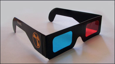
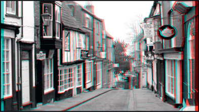
Figure 6.33 shows a stylish pair of anaglyph glasses and Figure 6.34 shows a typical anaglyph picture. If you have a pair of red and cyan anaglyph glasses lying around you can try them out on this picture and the following illustrations. The anaglyph process merges the two offset views into a single image with one view colored cyan and the other view color red. The red and cyan lenses of the anaglyph glasses then allow each eye to see its intended view while blocking the other eye.
The problems with anaglyph are ghosting, color degradation, and retinal rivalry (different brightness to each eye). It’s just not a very good way to present separate views to each eye, but it is incredibly cheap. In movie theaters high-tech polarizing display systems and glasses are used for their much better quality and low cost for a mass audience. However, in a production studio active shutter systems are most common. An active shutter system has rapidly blinking LCD glasses synchronized to a display (monitor) that is rapidly flicking between the left and right eye views. While the active shutter technology gives superior stereo viewing it is too expensive for mass distribution to a theater audience.
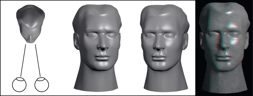
Figure 6.35
Two points of view result in stereopsis – the perception of depth
Stereopsis is the official term for the perception of depth in a scene due to viewing it from two points of view with our binocular vision. Figure 6.35 illustrates the idea with the resulting stereo image on the right. There are two components to our stereopsis – convergence and accommodation. Convergence is the inward rotation of the eyes to converge on a target, which is part of the data the brain uses to compute depth. Accommodation is the focusing of the eyes on the target, which is another part of the data the brain uses. The brain takes this data plus the images on the retina to achieve “fusion”, which is the process of merging the two views and matching their features to get depth perception. No fusion, no depth perception.
Stereo movies have an intrinsic problem in that they separate the convergence from the accommodation. In the real world when we look at an object our eyes converge at that distance then accommodate (focus) on it. Both the focus and convergence change together for objects near and far. But not in a stereo movie. The focus is fixed at the screen but the convergence changes as objects move in and out of the screen. This is an unnatural act and about 1 in 7 (15% of the audience) cannot do it. As stereo artists we must be concerned with not increasing this number by further abusing the human visual system with our stereo compositing – which is unfortunately easy to do if you do not understand the issues.
Stereoscopy, or the creation and display of stereo images, has its own technology and vocabulary, so there are a few concepts and terms that we need to become familiar with. Normal photography has one camera, or eye, to record a scene which produces a single “flat” picture (Figure 6.36). Stereoscopy uses two cameras to capture two views of the scene at slightly different angles to produce a stereo pair of images (Figure 6.37). If the stereo pair is projected in such a way as to present these slightly different views to each eye the illusion of depth will be introduced into the picture.

Figure 6.36
Mono view from one camera
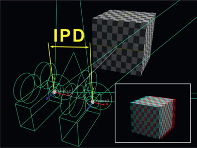
Parallax refers to the offset between the two views. If an object is close to the viewer the offset will be greater (more parallax) and if an object is far away the offset will be less (less parallax). Another thing that affects parallax is the interpupillary distance, which is the distance between our eyes which is around 2.5 inches for the average adult (64mm for Europeans). But for stereo cameras it is the distance between the center axis of their lenses. The interpupillary distance between the two stereo cameras in Figure 6.37 is marked as the “IPD”. Increasing or decreasing the interpupillary distance increases and decreases the parallax. Some refer to this camera separation distance as the interaxial distance (IAD), a reference to the distance between the optical axis of their lenses.
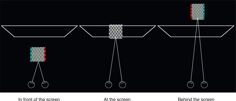
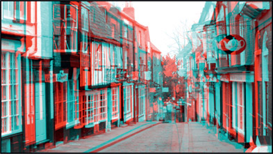
Disparity is the measure of the pixel offset for an object between the left and right views and is a key attribute of stereo compositing. Figure 6.38 illustrates how the disparity changes as an object starts in front of the screen then moves behind it. It also shows how the eyes change convergence with the apparent depth of the object, but again, the focal point is always the screen. The left example has the object in front of the screen (in “theater space”) and it exhibits a lot of disparity with the red view shifted to the right. The right example shows the object behind the screen (in “screen space”) and the red view is now shifted to the left. Note that the middle example shows the object at the screen plane so it has no disparity at all.
So parallax is the offset in the viewing angle for image capture, and disparity is its pixel offset in the digital image. The disparity is routinely adjusted when compositing stereo shots, but note this well – disparity is NOT the same as depth. You cannot use the depth Z data of a scene as the disparity data, though many try. They do have a mathematical relationship, but they are not the same and cannot be substituted for each other.
As we saw in the introduction section of stereo compositing some stereo projects are conversions from flat. When you consider the vast library of films waiting in the studio vaults it is clear that conversion will be a very important method of producing stereo films in the future. So let us take a look at the daunting process of conversion. Interestingly, it requires a fairly even mix of both 3D and compositing to convert a film to stereo.
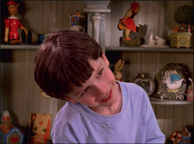
Some conversion processes use the unaltered original frames for the left eye then synthesize the right eye image. Other processes will actually isolate all of the elements in a shot and reconstruct both eyes. Let us consider the example in Figure 6.39. To make the right eye, the boy must be isolated, shifted left, then composited back over the background. You can see the offset in the boy’s position in Figure 6.40. Of course, to composite the right eye the background will have to be painted or composited to replace the exposed pixels that were originally covered by the boy. The problem is that the tiniest variation between the pixels of the two backgrounds creates a ghosting effect that can be uncomfortable to the eye. It turns out that it is actually much better to isolate the boy, make one clean background plate, and then composite two slightly offset boys over the same background plate. There are no discrepancies in the background so there are no artifacts. But this is obviously more time-consuming and expensive.
In the previous paragraph I glibly said, “the boy must be isolated”, which is obvious if an offset composite is to be made. Unfortunately, this is usually a Herculean task. Consider our boy in Figure 6.39. To start with, we will need a very tight roto around his outer edge. Since the wispy hairs cannot be rotoscoped they will either have to be painted or keyed. Keying is a serious problem because this is obviously not a greenscreen so it is a very difficult key and painting is both time consuming and difficult to appear natural. Keep in mind that this would be considered an easy shot. How about a couple dancing the jitterbug with flying skirts and hair? How about a mob scene? The isolation of objects is one of the most labor-intensive aspects of stereo conversion.
Once the rotos, keys, and painted masks are completed the next step is to layer the elements in depth. Figure 6.41 shows a high-angle view of the 3D arrangement to show how the shot is separated into layers. But wait, there’s more. If the layers are simply flat cardboard cutouts that’s exactly what they will look like when viewed in stereo. Each object must be projected onto a 3-dimensional mesh of some kind that can be contoured to give it a natural roundness like the illustration in Figure 6.42. The mesh shown here is actually oversimplified for illustration purposes. The real mesh would have much more detail to reflect the different depths of the eyes, nose, neck, and shirt. And, of course,
since the character would be moving around, this mesh must also be animated by hand to match. More labor intensive work.
And we are still not done. A new artist, the “stereographer”, now joins the project to perform “depth grading” where the relative depths of the various objects in the scene are dialed in. Depth grading is a high art with many artistic and technical issues to be aware of which we will now explore.
When compositing a stereo shot you may well have to be your own stereographer and perform the depth grading yourself. As mentioned above, one of the problems with stereo displays is that they are unnatural to the human eye. In the real world the eye adjusts to depth in a scene in two ways, convergence and accommodation (focus). Convergence is where the eyes rotate inward to meet at different distances depending on the distance to the item of interest. Focus is the lens of the eye focusing at different distances. The viewing screen of a stereo film or video is at a fixed distance from the viewer so there is no focus change. All of the depth information is due to convergence, and this is unnatural to the eye. Some viewers get eyestrain from this unnatural act. Following are some issues to be aware of when depth grading a stereo shot.
It is visually jarring to have a scene with the focal object popping out of the screen, then smash cut to the next scene where the focal object is far behind the screen. It is therefore an essential part of the depth-grading process to consider scene-to-scene transitions as well as the consistency of the depth placement of the same objects from scene-to-scene. There are also differing aesthetic schools of thought here, just like in other aspects of filmmaking. Some prefer to reduce the depth-of-field effects so the viewer can focus on whatever interests him in the scene, while others put in a large depth of field so that only the item of interest is in focus, to keep the viewer’s eyes where the director wants. Some want all focal elements to converge at the screen plane while others move things deeper into screen space.
The dashboard effect describes the difficulty in reconverging the eyes after an abrupt change in the scene depth. An example would be glancing back and forth from the dashboard of your car back to the horizon. It takes a moment for the visual system to adapt to the new depth. When depth grading a shot the previous and next shots must be taken into consideration to avoid jerking the audience’s eyes in and out of the screen with rapidly changing convergence.
If there absolutely must be a great difference in convergence between two shots then the depth grading can be subtly animated to gently shift the convergence over time – rather like a “follow focus” in a flat shot.
This is a perceptually disturbing phenomenon that occurs when an object is depth-graded to appear close to the viewer in theater space but is clipped by the frame edge. As it touches the frame edge one of the eyes will lose a portion of its view, which introduces a visual disparity that disturbs the viewer. The left and right edges of Figure 6.43 exhibit this problem as the buildings extend off the screen into theater space. The fix is to re-grade the depth to move the scene deeper into screen space so all of it appears to be behind the screen plane.
The reason this works is due to our pre-wired experience of looking out of a window. The outdoor scene is framed by the window but our brains ignore the disparity of the window frame as we focus on the far scene. This is what the re-graded depth duplicates in Figure 6.44 so that it appears natural.
Miniaturization occurs when the interaxial distance is exaggerated so much that objects in the scene somehow appear to be tiny. Great story here – I was bidding on a stereo project some years ago and the client was telling a ghastly tale about when they were making a stereo film with a flyover of the Grand Canyon. The director wanted to really exaggerate the stereo effect so the two cameras were mounted under a helicopter nearly 10 feet apart. The chopper flew over the Grand Canyon filming for hours but when the film was projected in stereo the Grand Canyon looked like a miniature toy set! Not exactly the mind-blowing effect the director had in mind. The brain knows the distance between our pupils and its relationship to the size of objects. Since the brain knows we don’t have 20-foot heads it decides that the Grand Canyon had to be very small. You can’t fool Mother Nature.
Convergence is when the eyes “toe in” to meet at some point in front of the viewer. When viewing something at infinity the eyes are essentially parallel. There are no natural situations where the eyes “toe out”. If the stereo disparity is set incorrectly the eyes can actually be forced to diverge, another very unnatural act.
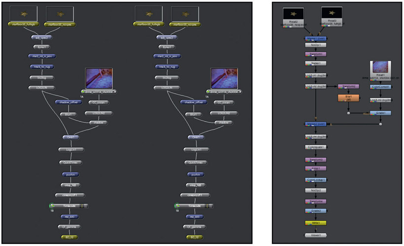
Some compositing programs support stereo workflows and others do not. Working on a stereo project with a compositing program that does not support stereo can be done, but it is very painful. It will require two parallel compositing node graphs, one for each eye, and you will have to constantly remember to duplicate every node setting between the two node graphs. If you adjust the blur of the left eye you must make an identical change to the right. A compositing program that supports a stereo workflow automatically updates the other eye for you. You can see a comparison of the node graphs from two different compositing programs in Figure 6.45. The pair of node graphs on the left illustrate how a shot is composited with a compositing program that does not support stereo, like Shake. The single node graph on the right illustrates how the same stereo shot is composited with Nuke, which does support stereo.
Since stereo compositing requires the development of two views for each shot there needs to not only be some efficient method of observing the stereo pair together but also a way to view them stereoscopically. Figure 6.46 shows a compositing viewer that can display the stereo pair side-by-side but can also quickly switch to an anaglyph presentation to aid in diagnostics and shot setup. Of course, if the compositing workstation has shutter glasses for stereo viewing rather than anaglyph, so much the better.
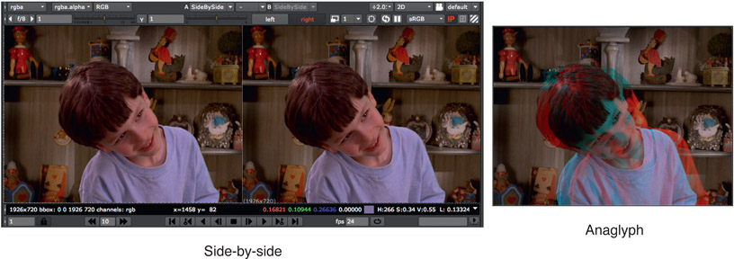
Figure 6.46
Viewing stereo images in the compositing program
While it is a major boost to productivity to make a change to one view and have the other view updated automatically, there are frequently situations where you want special treatment for just one view. For those situations the compositing program must support a “split and join views” feature that allows you to easily isolate one of the views for special processing.
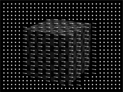
A disparity map documents how the pixels have shifted between the left and right views of the same frame (a stereo pair). Objects at the same depth as the screen will have not shifted at all, while objects in front of the screen in theater space will shift in one direction and objects behind the screen in screen space will shift in the opposite direction. Figure 6.47 shows the stereo pair of a simple object while Figure 6.48 shows the resulting disparity map. One view has been ghosted in just for reference. The arrows, or vectors, show the direction that the pixels shifted between the two views while the dots represent vectors of zero length where there was no shift at all. A disparity map does not actually show arrows. The pixel offsets are encoded in two image channels with one channel holding code values that indicate how far each pixel is shifted horizontally and the other channel how far vertically.
Disparity maps are generated by sophisticated software that performs a frame-by-frame feature-matching analysis of how the objects in the scene have shifted between the two views. The type of analysis it does is similar to optical flow. Where optical flow is interested in how objects move between frames, disparity maps are interested in how objects move between the two views of the same frame. So what can you do with a disparity map? A great deal, it turns out.
Rotoscoping – let’s say you need to rotoscope something. If you have a disparity map you can draw the roto for just one view then the disparity map will automatically shift a copy of the roto over for the other view.
Paint – perhaps something needs to be painted. The disparity map can automatically shift a copy of the brush strokes from one view to paint the other view.
Motion Tracking – you might need to do some motion tracking. You can motion track just one view then use the disparity map to shift the tracking data to correlate with the other view.
Disparity maps are a serious time-saver and a major productivity tool. However, they do tend to break down when dealing with semi-transparent pixels such as transparent objects, motion blurred edges, or fine hair detail. The reason is that a semi-transparent pixel holds information about two different objects, one in front and one in back, while the disparity map only holds information about one layer. It’s a problem.
This completes our tour of compositing techniques for greenscreen and bluescreen keying. In the next chapter we will focus on compositing CGI, another huge – and growing – staple of compositing visual effects. In the chapter we will see the proper techniques for compositing the various lighting passes for the CG objects, as well as look at important technologies such as camera tracking, camera projection, alembic geometry, and deep compositing.