The late Paleozoic ice age lasted for ~67 m.y. [million years] in eastern Australia, and as such, it was the longest-lived icehouse interval in the Phanerozoic.
—Fielding, Frank, Birgenheier, et al. (2008, 55)
ICE AGES IN EARTH HISTORY
We know that at least seven ice ages have occurred in the past 4,560 million years, time periods during which the Earth partially—or almost entirely—froze over. The history of the Earth is divided into four eons: the Hadean, Archaean, Proterozoic, and Phanerozoic, from oldest to youngest (for the geologic timescale, see table 1.1). These eons are themselves divided into smaller time units, the eras, and they are divided into still smaller time units, the periods (table 1.1), much as our calendar years are divided into months, weeks, and days. We know from fossil evidence that ancient bacterial life was present on the Earth 3,450 million years ago, during the Paleoarchaean Era, and we have geochemical evidence that indicates that life was present even earlier during the Eoarchaean Era, some 3,830 million years ago (McGhee 2013; Nutman et al. 2016). The first four of the known ice ages occurred during the Proterozoic Eon, much later in time than the appearance of life on Earth, and three more ice ages occurred even later during the Phanerozoic Eon; thus life on Earth has successfully survived them all—but at a cost. Many of the ice ages are associated with periods of extinction and large losses of biological diversity, a topic that will be explored in more detail in the next section of this chapter.
TABLE 1.1 The geologic timescale and ice ages.
| Eon |
Era |
Period |
Time of Onset (Ma) |
Ice Ages (ICE) |
| Phanerozoic |
Cenozoic |
Quaternary |
2.59 |
ICE |
| |
|
Neogene |
23.03 |
ICE |
| |
|
Paleogene |
66.0 |
ICE |
| |
Mesozoic |
Cretaceous |
145.0 |
|
| |
|
Jurassic |
201.3 |
|
| |
|
Triassic |
252.2 |
|
| |
Paleozoic |
Permian |
298.9 |
ICE |
| |
|
Carboniferous |
358.9 |
ICE |
| |
|
Devonian |
419.2 |
ICE |
| |
|
Silurian |
443.8 |
|
| |
|
Ordovician |
485.4 |
ICE |
| |
|
Cambrian |
541 |
|
| Proterozoic |
Neoproterozoic |
Ediacaran |
635 |
ICE |
| |
|
Cryogenian |
850 |
ICE |
| |
|
Tonian |
1,000 |
|
| |
Mesoproterozoic |
Stenian |
1,200 |
|
| |
|
Ectasian |
1,400 |
|
| |
|
Calymmian |
1,600 |
|
| |
Paleoproterozoic |
Statherian |
1,800 |
|
| |
|
Orosirian |
2,050 |
|
| |
|
Rhyacian |
2,300 |
ICE |
| |
|
Siderian |
2,500 |
|
| Archaean |
Neoarchaean |
|
2,800 |
|
| |
Mesoarchaean |
|
3,200 |
|
| |
Paleoarchaean |
|
3,600 |
|
| |
Eoarchaean |
|
4,000 |
|
| Hadean |
|
|
4,560 |
|
Source: Timescale modified from Gradstein et al. (2012).
Note: Ma = millions of years before the present for the start of each time unit listed.
A major difference between the four Proterozoic and three Phanerozoic glacial episodes is reflected in their formal names, given in table 1.2. The four Proterozoic episodes are called snowball Earths, whereas the three Phanerozoic episodes simply are called ice ages. The snowball-Earth glaciations were much more geographically extensive than any seen in the Phanerozoic in that continental-covering, sea-level-reaching ice sheets extended from the poles of the planet all the way down to the equator. From space, the entire planet may have looked like one giant snowball, hence the name “snowball Earth.” The first known snowball Earth, the Huronian, occurred some 2,300 million years ago during the Rhyacian Period (tables 1.1 and 1.2). Surprisingly, it is now thought that life may have triggered not only this massive freezing of the Earth during the Rhyacian but also the first mass extinction in Earth history. How could this be?
TABLE 1.2 Ice ages in Earth history.
| Ice Age |
Position in Geologic Time (table 1.1) |
| A. Phanerozoic ice ages: |
| 1. Cenozoic Ice Age |
Late Paleogene to Recent |
| 2. Late Paleozoic Ice Age |
Late Devonian to Late Permian |
| 3. End-Ordovician Ice Age |
Late Ordovician |
| B. Proterozoic ice ages: |
| 1. Gaskiers Snowball Earth |
Ediacaran |
| 2. Marinoan Snowball Earth |
Cryogenian |
| 3. Sturtian Snowball Earth |
Cryogenian |
| 4. Huronian Snowball Earth |
Rhyacian |
About 200 million years earlier than the Huronian freezing, at the beginning of the Siderian Period of the Paleoproterozoic Era (table 1.1), an event of major importance in the evolution of life on Earth occurred—the Great Oxygenation Event, or GOE for short. The very atmosphere of the Earth has been radically transformed by the presence of life. The original atmosphere of the Earth was probably very similar to that of its sister rocky volcanic planets Mars and Venus—that is, composed mostly of carbon dioxide. The atmosphere of Mars today is 95 percent carbon dioxide and the atmosphere of Venus is 97 percent, whereas the atmosphere of the pre-industrial-age Earth was only 0.03 percent carbon dioxide.1 Both anaerobic and aerobic photosynthesizing bacteria2 actively remove carbon dioxide from the atmosphere and use the carbon to form complex hydrocarbons for food. Thus, on Earth, life has been removing carbon dioxide from the atmosphere for the last 3,830 million years, contributing to the transformation of the Earth’s atmosphere to its present carbon-dioxide-depleted state.
The aerobic photosynthesizing cyanobacteria not only remove carbon dioxide from the atmosphere but also add oxygen to the atmosphere.3 About 2,500 million years ago, the oxygen-producing activity of the ancient cyanobacteria was finally to have its first major impact on the atmosphere of the Earth: it triggered the GOE. For the future evolution of complex—and large—life-forms with aerobic metabolism, the GOE was good news indeed as these organisms need free oxygen. For the ancient anaerobic life-forms—the original inhabitants of Earth—the GOE was a disaster because oxygen is a poison to them. The first mass extinction in the history of life on Earth probably occurred 2,500 million years ago, when vast unknown numbers of species of anaerobic bacteria and archaea perished by oxygen poisoning (McGhee 2013).
Diffusion of oxygen into the atmosphere was most probably the trigger of the Huronian Snowball Earth in the Rhyacian Period of the Paleoproterozoic Era (table 1.1), which occurred about 200 million years after the GOE (Lane 2002; Kopp et al. 2005). The steady drawdown of carbon dioxide, caused by the photosynthetic activity of life, was already reducing the greenhouse effect of this gas in the atmosphere. The presence of free oxygen in the atmosphere may then have begun to remove an even more powerful greenhouse gas—methane—via oxidation.4 The resulting sharp drop in the greenhouse capacity of the atmosphere of the Earth may have triggered this first great snowball in Earth history.
Some 300 million years later, in the Orosirian Period of the Paleoprotoerozoic Era (table 1.1), oxygen concentrations in the atmosphere had reached high enough levels to begin oxidizing iron on land, and the first redbed strata appear in the terrestrial rock record. Redbeds are just that: layered beds of red sandstones and shales in which the iron has been oxidized, giving the strata their characteristic rusty-red color. By this time, the aerobic photosynthetic activity of cyanobacteria had raised the amount of oxygen in the atmosphere to something between 1 and 4 percent.5
Much later, the Earth froze in three snowball phases in quick succession—quick on a geologic timescale (tables 1.1 and 1.2). Two of these phases, the Sturtian and Marinoan Snowball Earths, occurred at 717 and 640 million years ago, respectively, during the Cryogenian Period of the Neoproterozoic—an aptly named period as “cryogen” comes from the Greek for “beginning of freezing cold.”6 The Sturtian Snowball Earth lasted some 57 million years; the Marinoan, about five million years; and the last snowball Earth, the Gaskiers, began 580 million years ago but lasted only 340,000 years during the Ediacaran Age (table 1.1).7
The earliest soft-tissued marine animals evolved about 780 million years ago (Erwin et al. 2011) during the Cryogenian, but it was only 541 million years ago that the first marine animals with mineralized tissues—skeletons—evolved. This evolutionary event marks the beginning of the Phanerozoic Eon (table 1.1), the geologic eon of the “visible animals.”8 The event is also often called the Cambrian Explosion, in recognition of the evolutionary pulse in the diversification of animal life that occurred at the beginning of the Cambrian Period of the Paleozoic Era (fig. 1.1). Large macroscopic animals with skeletons made of calcium, silica, and phosphorous compounds suddenly are present in rocks that previously contained only the impressions made by a few types of soft-bodied animals. All in all, almost 100 families of marine animals originated in the pulse of diversification that occurred at the beginning of the Paleozoic Era.
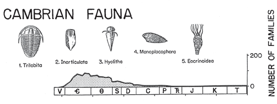
FIGURE 1.1 An evolutionary pulse in the diversification of large-bodied animals with skeletons occurred in the early Cambrian (graph); illustrated are some of the characteristic skeletonized marine animals of the Cambrian fauna (see text for discussion). Geologic timescale abbreviations: V, Ediacaran; barred-C, Cambrian; Ө, Ordovician; S, Silurian; D, Devonian; C, Carboniferous; P, Permian; TR, Triassic; J, Jurassic; K, Cretaceous; T, Tertiary (Paleogene and Neogene).
Source: From Paleobiology, volume 10, pp. 246–267, by J. J. Sepkoski Jr., “A Kinematic Model of Phanerozoic Taxonomic Diversity: III. Post-Paleozoic Families and Mass Extinctions,” copyright © 1984 The Paleontological Society. Reprinted with permission of Cambridge University Press.
Figure 1.1 illustrates some of the early skeletonized members of the major evolutionary clades of animals that were to become characteristic of the Paleozoic marine world: the Arthropoda (trilobites), Lophophorata (inarticulate brachiopods, hyoliths9), Mollusca (monoplacophorans), and Echinodermata (eocrinoids). We will examine the ecology and further evolution of all of these animal groups in greater detail in the chapters that follow. For example, the lophophorates are of particular interest in that they were later to evolve gigantic brachiopod shellfish in the Carboniferous.
Why did so many types of large animals with different skeletal chemistries appear so suddenly in the fossil record? A clue may be seen in some modern-day animals, such as bivalve molluscs that have the capacity to switch from aerobic metabolism to anaerobic metabolism when the oxygen content in water becomes depleted. While in the anaerobic-respiration mode, these bivalves also produce acid metabolites as a byproduct, and these acids actually begin to etch away and dissolve the calcium-carbonate shell of the animal (Lutz and Rhoads 1977; Babarro and De Zwaan 2008). Thus it has been proposed that the ability to grow and maintain mineralized skeletal tissues is a trait that is found in the aerobic-respiring organisms, meaning there has to be enough oxygen present in the environment to allow organisms to respire aerobically. Atmospheric modeling of the evolution of the Earth’s atmosphere indicates that around 540 million years ago, just before the dawn of the Cambrian, oxygen levels in the atmosphere had finally risen to around 16 to 18 percent (Berner 2006), as compared to present-day levels of 21 percent. (We will consider these models in detail in chapters 3 and 4.) Atmospheric oxygen levels of 16 to 18 percent may have been the final trigger for animals belonging to numerous disparate phylogenetic lineages to simultaneously achieve sustained aerobic respiration, increase in size, and secrete mineralized skeletal tissues of several different chemical compositions in the different lineages. After the GOE and the Huronian Snowball Earth, the fact that the planet was hit by at least three more snowball-Earth glaciations in the latest Neoproterozoic (tables 1.1 and 1.2), immediately before the Cambrian animal diversification, is evidence for the continued effects of the drawdown of the greenhouse-gas carbon dioxide from the atmosphere and the injection of oxygen into the atmosphere by aerobic photosynthetic life.
In contrast to the snowball Earths, only the poles and higher-latitude regions of the Earth were covered by ice in the three Phanerozoic ice ages (tables 1.1 and 1.2). Our modern world is the product of the Cenozoic Ice Age, and polar ice and high-latitude continental glaciation still exist on the Earth—but perhaps not for long. The Cenozoic Ice Age began about 34 million years ago in the late Paleogene,10 and its last glacial interval ended about 10,000 years ago (Lewis et al. 2008). It remains to be seen whether the Earth is still in the Cenozoic Ice Age or our warmer modern world is merely a interglacial interlude and whether the great ice sheets will return in the near future (on a geologic timescale). An alternative view is that the Earth is now in a major and unusual warming phase, triggered by the injection of carbon dioxide into the atmosphere by the human burning of fossil hydrocarbons for fuel. Humans began to mine and burn coal strata—the overwhelming majority of which are Carboniferous in age—in a big way during the Industrial Revolution and later added oil and natural-gas extraction and combustion through subsurface drilling. The subsequent increase in the carbon dioxide content of the atmosphere parallels an increase in the atmospheric temperature of the Earth, resulting in the accelerated melting of the residual ice that still exists from the last glacial phase of the Cenozoic Ice Age. Continued warming may result in an ice-free hot Earth in the future, and the Cenozoic Ice Age will be history.
The first Phanerozoic glacial phase, the end-Ordovician Ice Age, was peculiar in that it occurred during a period in geologic time when the Earth was in a long-term greenhouse phase and was quite warm, with an atmosphere still rich in carbon dioxide. The ice age was also quite short, consisting of an intense glaciation phase that lasted only 1.9 million years within a longer-term period of glacial advances and retreats in the latter part of the Ordovician and early part of the Silurian (McGhee et al. 2012, 2013). The evolution of the first land plants from water-dwelling plants had occurred by the middle of the Ordovician, but by the end of the Ordovician the continents of the Earth were still populated only by very small liverworts and related simple plants. The Ordovician is sometimes called the “Lilliputian plant world” because these tiny land plants—averaging under three centimeters (a little over an inch) in height—constituted the only plant cover of the planet Earth at that time. A few multilegged marine animals occasionally ventured out of the oceans onto the tidal flats and dry land near the end of the Ordovician—we have their fossil footprints preserved in stone—but they quickly returned to water and did not live on the land. (For an extensive discussion of the invasion of land by plants and animals, see McGhee 2013.) And last, in the south polar region of the planet, a vast ice sheet covered at least 30 million square kilometers (almost 12 million square miles) of land (Sheehan 2001); otherwise the land areas of the Earth were empty.
This book is about the second of the Phanerozoic glacial episodes (tables 1.1 and 1.2), the Late Paleozoic Ice Age—the longest ice age on Earth for the past 541 million years since the pulse of diversification of complex animal life in the Cambrian Explosion. If the world of the Ordovician Ice Age seems strange, the world of the Late Paleozoic Ice Age was far stranger, as we will see in this book.
ICE AGES AND EXTINCTIONS
All of the Phanerozoic ice ages (and probably all of the snowball Earths) are associated with the extinction of large numbers of species and major losses of biodiversity—but not all biodiversity crises in Earth history are associated with ice ages. Of the eight largest Phanerozoic biodiversity crises, five are argued to have been related to ice ages—one with the short end-Ordovician Ice Age and the other four with the longest glaciation in the Phanerozoic, the Late Paleozoic Ice Age (table 1.3). Curiously, these are also the first five biodiversity crises in Phanerozoic history (table 1.4) since the Great Ordovician Biodiversification Event (GOBE) (Webby et al. 2004; Servais et al. 2010), the second massive diversification of animal life in the oceans following the Cambrian Explosion (we will consider the evolutionary significance of the GOBE in detail in chapter 6). Just as curious is the fact that the end-Permian, end-Triassic (table 1.4), and end-Cretaceous biodiversity crises were clearly not associated with ice ages. We will consider the causes of the end-Permian mass extinction—the largest in Earth history—in detail in chapter 6, along with the end-Triassic extinction, as these two catastrophes appear to have had a similar causal mechanism. The end-Cretaceous mass extinction—the event that destroyed the dinosaur ecosystem—is now generally attributed to the effects of the impact of the massive asteroid that produced the 180-kilometer-diameter (112-mile-diameter) Chicxulub Crater in Mexico and thus had an extraterrestrial cause, not an Earthly one.
TABLE 1.3 Ecological-severity ranking from most severe (#1) to least severe (#7) of the eight largest Phanerozoic biodiversity crises since the beginning of the Ordovician.
| #1. End-Permian (Changhsingian Age) |
| #2. End-Cretaceous (Maastrichtian Age) |
| #3. End-Triassic (Rhaetian Age) |
| #4. Late Devonian (Frasnian Age) |
| #5. End-Middle Permian (Capitanian Age) |
| #6. Early Carboniferous (Serpukhovian Age) |
| #7. End-Devonian (Famennian Age), End-Ordovician (Hirnantian Age) |
Source: From McGhee et al. (2004, 2013).
Note: The four biodiversity crises that are thought to be related to the Late Paleozoic Ice Age are listed in bold type; see text for discussion.
TABLE 1.4 Epoch and age divisions of the geologic timescale in the critical time interval leading up to and immediately following the Late Paleozoic Ice Age.
| Period |
Epoch |
Age |
Time of Onset (Ma) |
Time of Crises |
| Jurassic (pars) |
|
Hettangian |
201.3 |
|
| Triassic |
Late |
Rhaetian |
209.5 |
← Biodiversity Crisis |
| |
|
Norian |
228.4 |
|
| |
|
Carnian |
237 |
|
| |
Middle |
Ladinian |
241.5 |
|
| |
|
Anisian |
247.1 |
|
| |
Early |
Olenekian |
250.0 |
|
| |
|
Induan |
252.2 |
|
| Permian |
Late |
Changhsingian |
254.2 |
← Biodiversity Crisis |
| |
(Lopingian) |
Wuchiapingian |
259.8 |
|
| |
Middle |
Capitanian |
265.1 |
← Biodiversity Crisis |
| |
(Guadalupian) |
Wordian |
268.8 |
|
| |
|
Roadian |
272.3 |
|
| |
Early |
Kungarian |
279.3 |
|
| |
(Cisuralian) |
Artinskian |
290.1 |
|
| |
|
Sakmarian |
295.5 |
|
| |
|
Asselian |
298.9 |
|
| Carboniferous |
Late |
Gzhelian |
303.7 |
|
| |
(Pennsylvanian) |
Kasimovian |
307.0 |
|
| |
|
Moscovian |
315.2 |
|
| |
|
Bashkirian |
323.2 |
|
| |
Early |
Serpukhovian |
330.9 |
← Biodiversity Crisis |
| |
(Mississippian) |
Visean |
346.7 |
|
| |
|
Tournaisian |
358.9 |
|
| Devonian |
Late |
Famennian |
372.2 |
← Biodiversity Crisis |
| |
|
Frasnian |
382.7 |
← Biodiversity Crisis |
| |
Middle |
Givetian |
387.7 |
|
| |
|
Eifelian |
393.3 |
|
| |
Early |
Emsian |
407.6 |
|
| |
|
Pragian |
410.8 |
|
| |
|
Lochkovian |
419.2 |
|
| Silurian |
Late |
Pridolian |
423.0 |
|
| |
|
Ludfordian |
425.6 |
|
| |
|
Gorstian |
427.4 |
|
| |
Middle |
Homerian |
430.5 |
|
| |
|
Sheinwoodian |
433.4 |
|
| |
Early |
Telychian |
438.5 |
|
| |
|
Aeronian |
440.8 |
|
| |
|
Rhuddanian |
443.8 |
|
| Ordovician |
Late |
Hirnantian |
445.2 |
← Biodiversity Crisis |
| |
|
Katian |
453.0 |
|
| |
|
Sandbian |
458.4 |
|
| |
Middle |
Darriwilian |
467.3 |
|
| |
|
Dapingian |
470.0 |
|
| |
Early |
Floian |
477.7 |
|
| |
|
Tremadocian |
485.4 |
|
Source: Timescale modified from Gradstein et al. (2012).
Note: The temporal position of the seven major biodiversity crises (table 1.3) that occurred in this time interval are indicated with arrows. Ma = millions of years before the present for the start of each time unit listed.
The short-lived end-Ordovician Ice Age triggered a mass extinction of marine species but had little effect on life on land simply because there was not much life on land to be affected (McGhee 2013). My colleagues Peter Sheehan, Dave Bottjer, Mary Droser, and Matthew Clapham and I have conducted comparative paleoecological analyses that have revealed that the environmental degradation produced by the end-Ordovician glaciation precipitated a major loss of marine biodiversity, yet the extinction failed to eliminate any key taxa or evolutionary traits and was of minimal ecological impact (Droser et al. 2000; McGhee et al. 2004, 2012, 2013). In terms of ecological severity, the end-Ordovician extinction had an impact equivalent to that of the end-Devonian extinction (table 1.3), and both extinctions were triggered by an intense glacial phase that was of a geologically short duration—1.9 million years in the end-Ordovician Hirnantian Age and 1.4 million years in the end-Devonian Famennian Age (McGhee et al. 2013; McGhee 2013).
In contrast to the end-Ordovician and end-Devonian biodiversity crises, the glaciation in the Early Carboniferous Serpukhovian Age triggered a precipitous drop in the speciation rate of marine species but only moderate diversity losses. However, the ecological impact of those diversity losses and ecosystem restructuring was an ecological level of magnitude larger than that seen in the end-Ordovician or end-Devonian extinctions (table 1.3) (McGhee et al. 2012). We will examine the sequence of Early Carboniferous evolutionary events and glaciation phases in more detail in chapter 2.
In contrast to all of the biodiversity crises considered thus far, the extinctions that occurred in the Capitanian Age at the end of the Middle Permian Epoch (tables 1.3 and 1.4) were associated with the waning of the Late Paleozoic Ice Age, not with its onset or expansion. The end of the Late Paleozoic Ice Age was triggered by the start of a major phase of global warming, and at the end of the Paleozoic Era occurred the end-Permian mass extinction, the most ecologically severe biodiversity crisis in the entire Phanerozoic—a truly global “Category 1” ecological crisis in both the Earth’s marine and terrestrial biota (McGhee et al. 2004; Cascales-Miñana et al. 2015). We will consider the dire consequences of these two Permian biodiversity crises in greater detail in chapters 5 and 6.
This leaves the enigmatic Late Devonian biodiversity crisis—so called because it occurred within the Late Devonian Epoch at the end of the Frasnian Age (tables 1.3 and 1.4). The Late Devonian crisis was a very severe event, in terms of both the magnitude of biodiversity loss and the ecological impact. It has the highest ecological severity of any of the biodiversity crises associated with a Phanerozoic ice age—if it was associated with a Phanerozoic ice age! We will consider the relationship of the Late Devonian biodiversity crisis to the Late Paleozoic Ice Age in great detail in the section “The Onset of the Late Paleozoic Ice Age?” later in this chapter.
Finally, the reader will have noticed that the Cenozoic Ice Age (table 1.2) is not listed in the ecological-severity ranking of biodiversity crises in table 1.3. Does this mean that no extinction or loss of biodiversity occurred during the Cenozoic Ice Age? No, significant extinctions are associated with the Cenozoic Ice Age, and we will also consider them in more detail in the “The Onset of the Late Paleozoic Ice Age?” section. In general, however, the biodiversity losses that occurred during the Cenozoic Ice Age were of much less magnitude than those associated with the Paleozoic crises. Why? Steve Stanley, a University of Hawaii paleontologist, has proposed an answer to that question: the biota of the Paleozoic world was more prone to extinction than the biota of the Cenozoic, a phenomenon revealed in the classic analyses of the University of Chicago paleontologists Dave Raup and Jack Sepkoski that demonstrate that the mean extinction rate of marine animals has declined through time; that is, Paleozoic marine species had a much higher rate of extinction than Cenozoic marine species (Raup and Sepkoski 1982; Stanley 2007). This phenomenon is not unexpected: the theory of natural selection would predict the evolution of increasing extinction resistance with time. In the Paleozoic, the biota was dominated by ancient species with higher extinction rates than modern species. For example, Stanley has shown that in the Late Devonian extinction, the older species lineages suffered extinction at a 20 percent higher rate than the more recently evolved species lineages, and as the majority of the Late Devonian species belonged to these older lineages, the total extinction rate was predictably high (Stanley 2007). In contrast, Cenozoic marine species are much more resistant to extinction, hence the total extinction rates seen in the Cenozoic Ice Age are predictably lower than those seen in the Late Paleozoic Ice Age. We will examine further evolutionary and ecological differences between the ancient Paleozoic species and the more modern Cenozoic species in more detail in chapter 6.
THE MYSTERY OF THE ICE AGES
What triggered these ice ages and snowball Earths in geologic time? Why did huge areas of the Earth become frozen in the past? Obviously, if the entire planet gets colder, it must somehow either not be receiving enough heat from the sun to maintain its previous temperature or be losing much more of its heat to space than previously or both.
The Earth does generate some of its own heat by the decay of radioactive minerals in its rocks, but the planet really depends upon electromagnetic radiation—light—from the nearest star, our sun, for heat. The sun is actually becoming hotter with time as it slowly burns more and more of its original hydrogen gas in the fusion production of helium. A cooler sun during the Proterozoic Eon may have contributed in part to the intensity of the snowball-Earth glaciations. In the past 541 million years, however, our models of the sun’s energy production predict no major fluctuations that could have triggered the Phanerozoic ice ages.
If the production of energy by the sun has been relatively constant for the past 541 million years, then one way to change the amount of heat that the Earth receives is to change the distance of the Earth from the sun: a planet closer to the sun receives more energy per unit area than a planet farther away. Although it is not apparent to us on human timescales, the Earth’s distance from the sun actually does vary on geologic timescales. The shape of the Earth’s orbit around the sun changes with time, from being almost a perfect circle to being stretched out into an ellipse—a shape variation that is known as orbital eccentricity (table 1.5). When the Earth’s orbit is nearly circular, the planet absorbs about the same amount of heat from the sun throughout the year, as the distance of the Earth from the sun—the radius of the circular orbit—does not change during the year. At the other extreme the Earth’s orbit is highly elliptical, with a long axis and a short axis. Twice a year the Earth is located at the short axis of the ellipse and warms up as it is closer to the sun, and twice a year the Earth is located at the long axis of the ellipse and cools down as it is farther from the sun. The stretching of the Earth’s orbit from a near circle to an ellipse and its rounding back to a circle again is a function of the gravitational influence of the other planets in the solar system, and it occurs periodically in cycles of 100,000 and 400,000 years of geologic time.
TABLE 1.5 Periodic orbital phenomena that affect the Earth’s climate.
| Phenomenon |
Periodicity of phenomenon |
| 1. Orbital Eccentricity: variation in the shape of the Earth’s orbit, from near-circular at one extreme to elliptical at the other. |
100,000 years and 400,000 years |
| 2. Rotational Axis Obliquity: variation in the tilt of the Earth’s spin axis, from a tilt of 22.1° at one extreme to 24.5° at the other. |
41,000 years |
| 3. Rotational Axis Precession: circular variation in the orientation of the Earth’s spin axis, from pointing to Polaris as the north pole star at one extreme to pointing in the opposite direction, along an arc of 180°, at the other. |
19,000 years and 23,000 years |
The Earth also experiences variation in solar radiation in two ways that are caused by its orientation relative to the sun, not its distance. The first of these, rotational axis obliquity, refers to the fact that the degree of tilt in the Earth’s rotational axis is not constant. The spin axis of the Earth is not vertical; that is, the planet tilts over on its side as it rotates. This tilt is responsible for the four seasons that we experience. For example, when the Northern Hemisphere of the Earth is tilted toward the sun, it receives more energy per unit area and is thus hotter—the summer season—than when it is tilted away from the sun and is thus colder—the winter season. The tilt in the rotational axis of the Earth varies between 22.1° and 24.5°. When the spin axis of the Earth is tilted over at 24.5°, the seasonal differences in temperature are much more pronounced—the winters are colder and the summers are hotter—than when the planet is tilted at only 22.1°. The degree of tilt of the Earth’s rotational axis oscillates in a 41,000-year cycle in geologic time. Finally, the direction in which the rotational axis of the Earth points varies with time—a phenomenon known as rotational axis precession. Simply expressed, the Earth wobbles with time like a toy top winding down, with its tilted-over rotational axis spinning around and around in a circle. The tilt of the Earth relative to the sun changes on 23,000- and 19,000-year cycles; thus, the Northern Hemisphere is now tilted toward the sun (summer) in June, but 23,000 years from now it will be tilted away from the sun (winter) in June.
To make things even more interesting, these three cycles—orbital eccentricity, axial obliquity, and axial precession—interact to magnify or diminish one another’s effect. For example, when the Earth is located farthest from the sun on an elliptical orbit (aphelion) and its axis is tilted over at 24.5° and is positioned at one of the solstices, the planet will become quite cold in one hemisphere and even the equator will cool. The opposite effect occurs when the Earth’s orbit is more circular, its axis is tilted at only 22.1°, and the equinoxes occur at aphelion. These orbital oscillations are called Milankovitch cycles, after the Serbian geophysicist Milutin Milankovitć (usually anglicized to Milankovitch in the English literature) who first proposed them. It has been demonstrated that the Earth’s climate did indeed vary in Milankovitch cycles of 400, 100, 41, 23, and 19 thousand years during the Cenozoic Ice Age (Zachos et al. 2001), and the 400- and 100-thousand-year eccentricity cycles have been detected in Late Carboniferous strata during the Late Paleozoic Ice Age (Heckel 2008; Horton et al. 2012).
However, the Milankovitch cycles in climate change became apparent only after the Cenozoic Ice Age had started and glaciers had formed on the Earth. Thus it appears that some stronger cooling mechanism is necessary to chill the planet down to form glaciers, which then wax and wane on weaker Milankovitch thermal frequencies. The next suspect in the ice ages mystery is changes in the Earth’s atmosphere—specifically, changes in the amount of the greenhouse gases carbon dioxide (CO2) and methane (CH4) in the atmosphere. These gases act much like the glass roof of a greenhouse (hence the name greenhouse gas): the glass roof allows higher-frequency sunlight to penetrate down into the greenhouse, where the light is absorbed by the plants and then radiated back as lower-frequency infrared light, but then the glass roof blocks the escape of the infrared light and thus causes the temperature within the greenhouse to become hotter and hotter. Likewise, given the same amount of energy received from the sun, the Earth will retain more of that energy as heat when the atmosphere of the planet is enriched with carbon dioxide and methane and will lose more of that energy back to space when the atmosphere contains little carbon dioxide and methane.
Thus, to cool the planet and initiate an ice age, the amount of greenhouse gases in the Earth’s atmosphere must be reduced (Montañez and Poulsen 2013). Carbon dioxide is removed from the atmosphere by two principal mechanisms: biological photosynthesis11 and chemical weathering of silicate rocks.12 Of these two processes, the chemical weathering of silicate rocks appears to be the more important: it is estimated that of the carbon dioxide that was removed from the Earth’s atmosphere during the Phanerozoic, about 80 percent was removed by silicate weathering and only about 20 percent by biological photosynthesis (Raymo and Ruddiman 1992). Carbon-dioxide removal by weathering is enhanced by the uplift and exposure of large surface areas of silicate rock to the Earth’s atmosphere during mountain-building events (Raymo and Ruddiman 1992) and by the exposure of silicate rocks in the equatorial humid zone of the Earth where the combination of high precipitation and high temperature intensifies the process of chemical weathering (Kent and Muttoni 2008; Irving 2008). Methane is removed from the atmosphere chiefly by oxidation, but the oxidation of methane then produces carbon dioxide,13 so we are back to the mechanisms of atmospheric carbon-dioxide removal in order to trigger global cooling.
The role of tectonic-forcing mechanisms of widespread mountain-building events (crustal buckling and uplift caused by collisions of continental plates, accretion of island-arc terranes onto continental plates, and subduction of oceanic plates under the margins of continental plates) and continental positionings (large number of continental plates located in the equatorial humid zone) in removing carbon dioxide from the Earth’s atmosphere via chemical weathering has been implicated in all of the known glaciations, from the four snowball-Earth glaciations in the Proterozoic (Melezhik 2006) to the end-Ordovician (Lenton et al. 2012), Cenozoic (Raymo and Ruddiman 1992; Zachos et al. 2001; DeConto and Pollard 2003; Kent and Muttoni 2008), and Late Paleozoic ice ages in the Phanerozoic. However, it has been argued that atmospheric carbon-dioxide depletion by biological evolutionary processes was also a significant contributing factor in triggering the Huronian Snowball Earth (the evolution of aerobic photosynthesis) (Kopp et al. 2005), the end-Ordovician Ice Age (the evolution of land plants) (Lenton et al. 2012), and the Late Paleozoic Ice Age (the evolution of forests) (Algeo et al. 1995, 2001).
The topic of this book is the Late Paleozoic Ice Age, so let us take a closer look at the proposed triggers of this climatic event. The Late Devonian was clearly a time of major tectonic activity. In the short time span (on geologic timescales) of only four million years during the Frasnian Age, major mountain-belt deformation and uplift spread across the Appalachian-Caledonian mountain chain in North America and Europe (then joined together in a single continent called Laurussia; see fig. 1.2) and further to the south in the Variscide mountain chain extending into northern Africa (on the giant southern supercontinent Gondwana; see fig. 1.2). These crustal deformations and mountainous uplifts were driven by the incipient collision of the southeastern margin of Laurussia (southeast North America) and the northwestern margin of Gondwana (northwest Africa). On the northeastern margin of Laurussia, mountainous uplifts occurred in the Ural mountain belt (western Russia), driven by the collision of the Kazakhstan crustal block with Laurussia, and to the east of that, the Central Asian mountain belt buckled and uplifted in the collision of the Siberian crustal block (eastern Russia) with the eastern margin of the Kazakhstan block. In terms of tectonic plate collisions, the Frasnian Age was a time of a multicar pileup on the geologic turnpike.

FIGURE 1.2 Paleogeography of the Earth in the late Frasnian Age. Lighter shaded areas surrounding the continents are shallow continental marine waters, and deep oceanic waters are black. The large continent straddling the equator in the left-center is Laurussia (modern-day North America and Europe), the smaller continent to the northwest of Laurussia is northern Asia, the islands east of Laurussia are pieces of eastern Asia, and the giant continent to the south of Laurussia is Gondwana (modern-day South America, Africa, India, Antarctica, and Australia all joined together).
Source: Global Paleogeography and Tectonics in Deep Time © 2016 Colorado Plateau Geosystems Inc. Reprinted with permission.
But that was not all. On the northwestern margin of Laurussia, crustal buckling and uplift occurred in the Antler mountain belt (western margin of the United States and Canada) eastward into the Ellesmerian-Svallbardian mountain belt (northern Canada). This deformation and uplift was triggered not by continental block collisions but rather by oceanic subduction and accretion of island-arc terranes along the northwestern margin of Laurussia. Nor was that all. To the south, on the giant continent Gondwana, similar oceanic-plate subduction and island-arc terrane accretion occurred in the Bolivianide mountain belt on the western margin of Gondwana (western South America) and in the Lachlan mountain belt on the eastern margin of Gondwana (eastern Australia and Antarctica). In summary, the Late Devonian Epoch was a period of intense tectonic activity on a global scale. (For a detailed discussion of the tectonic events that occurred during the Late Devonian, see McGhee 2013.)
Finally, there exists the possibility that yet another major tectonic mechanism might have been active in the Late Devonian—mantle-plume volcanism. In mantle-plume volcanism, a giant plume of magma rises from deep in the Earth’s mantle and, when it intersects continental crust at the Earth’s surface, erupts in huge volumes of basaltic lava—the weathering of which could extract huge volumes of carbon dioxide from the atmosphere. Possible evidence for mantle-plume volcanism comes from the Viluy igneous province in eastern Siberia (Courtillot and Renne 2003; Courtillot et al. 2010; Bond and Wignall 2014). The original size of the Viluy igneous province is unknown because it is highly eroded. Estimates suggest that the extent of these lava flows may have been as much as six million square kilometers (2.3 million square miles). Radiometric dating of the Viluy lavas is not precise, but it does place the eruptions in the interval of 377 to 350 million years ago—that is, sometime from the middle Frasnian Age in the Late Devonian to the late Tournaisian Age in the Early Carboniferous (table 1.4). Smaller igneous provinces, some with kimberlite14 magmatism that demonstrates a mantle source for the volcanism, are also known in other areas of the ancient Laurussian continent from the same time interval; thus, there may have been several areas of mantle-plume volcanism active in the Late Devonian (Racki and Wignall 2005).
The uplift, deformation, and exposure to the atmosphere of huge surface areas of silicate rocks that occurred in the Late Devonian tectonic events should have triggered a massive drawdown of carbon dioxide from the atmosphere caused by the chemical weathering of these newly exposed rocks. In addition, the Laurussian continental block was positioned directly on the equator within the equatorial humid zone of the Earth in the Frasnian (fig. 1.2), thus enhancing the chemical weathering of silicate rocks located in this region. Thus, it is not unexpected that these potential carbon-dioxide-depleting tectonic mechanisms for triggering global cooling have been proposed as causes not only of the end-Famennian glaciation but also of a hypothesized glaciation that may have occurred at the end of the Frasnian as well (Averbuch et al. 2005). In addition, the University of Lille sedimentologist Olivier Averbuch and his colleagues have offered an independent geochemical line of evidence in support of the chemical-weathering hypothesis for global cooling in the Late Devonian: ratios of the isotopes strontium-87 and strontium-86 in seawater. Strontium-87 is radiogenic and is primarily found in continental rocks; strontium-86 is nonradiogenic and is primarily found in seafloor rocks. Thus higher ratios of strontium-87 to strontium-86 indicate higher rates of chemical weathering and erosion of crustal rocks on the continents, with the delivery of more strontium-87 to the oceans; lower ratios indicate the reverse (or increased seafloor hydrothermal activity). Strontium-87 to strontium-86 ratios increased during the Frasnian Age and spiked in the late Frasnian, indicating an intensification of continental weathering at this critical time. A second spike in strontium-87 to strontium-86 ratios occurred some five million years later in the early Famennian, indicating a second pulse of intense continental weathering at this time (Averbuch et al. 2005). Did these periods of intense weathering of continental silicate rocks deplete the Earth’s atmosphere of enough carbon dioxide to trigger the formation of glaciers in the late Frasnian and early Famennian?
Another continental positioning (other than equatorial) also contributed to the formation of glaciers during the Late Devonian: the giant continent Gondwana was definitely positioned over the South Pole of the Earth in the late Famennian, 360 million years ago (fig. 1.3). Over the next 110 to 115 million years the geographic position of the South Pole on Gondwana shifted eastward across the landmass, from South America to Africa to Antarctica to Australia (fig. 1.3), as the giant tectonic plate holding Gondwana slowly moved westward over the South Pole. In the Cenozoic Ice Age the continent Antarctica was positioned over the South Pole (where it still is today); it has an ice-covered surface area of 13.72 million square kilometers (5.30 million square miles). In the Late Paleozoic, the giant continent Gondwana had a surface area of 74.23 million square kilometers (28.65 million square miles), almost five-and-one-half times bigger than Antarctica. Gondwana was so large that it was never entirely covered by ice during the Late Paleozoic Ice Age; rather, the centers of multiple glacial masses migrated across the giant continent in concert with its movement over the South Pole (fig. 1.3).

FIGURE 1.3 Polar wandering path across Gondwana from 360 million years ago to 250 million years ago. Also shown are the geologic outcrop areas of glacial strata, where Glacial I strata are Late Devonian to Early Carboniferous in age, Glacial II strata are late-Early to Late Carboniferous in age, and Glacial III strata are Early to Middle Permian in age.
Source: From Geological Society of America Special Paper 441, pp. 331–342, by T. D. Frank et al., “Paleozoic Climate Dynamics Revealed by Comparison of Ice-Proximal Stratigraphic and Ice-Distal Isotopic Records,” copyright © 2008 Geological Society of America. Reprinted with permission.
Independent biological weathering events also may have contributed to atmospheric carbon-dioxide depletion during the Devonian. A major event in the evolution of land plants occurred in the Givetian Age of the Middle Devonian—the first forests on Earth—and the evolution of forests certainly had to have added to the tectonic effects triggering global cooling. The Earth’s oldest known forest is the famous Gilboa fossil forest of New York State; it consisted of trees that were large cladoxylopsids, extinct relatives of our modern-day ferns. (Tree ferns still exist today, such as the Australian tree fern Cyathea cooperi.) In the Givetian, the cladoxylopsid fernlike tree was the species Wattieza (Eospermatopteris) erianus, which stood more than eight meters (26 feet) tall and had trunks that were a half-meter to a meter (1.6 to 3.3 feet) in diameter. Yet these same large trees were anchored only by a broad, bulbous base that had numerous small, short roots.
The next step in the evolution of trees was the appearance of forests of giant Archaeopteris trees in the Frasnian Age of the Late Devonian. Unlike the fernlike cladoxylopsid trees, Archaeopteris trees were lignophytes—true woody trees with strong trunks; they towered 30 meters (100 feet) into the air and had deep, branched root systems that penetrated over a meter (3.3 feet) into the ground. These trees produced deep soil horizons by both chemical and mechanical weathering of the rocks into which they were rooted. However, the Archaeopteris trees still reproduced by spores, not seeds like our modern lignophyte trees, and they were generally restricted to the wetlands in the lowland areas of the Earth because they needed a reliable source of water for their reproduction by spore.
The final step in the evolution of trees was the appearance of the first seed-reproducing plants, the spermatophytes. The first spermatophyte lignophyte trees evolved in the Famennian Age and, not needing water in reproduction, colonized the dry highlands and mountains that were out of reach for non-spermatophyte Archaeopteris trees. Thus, huge areas of exposed silicate rock were now within reach of the seed plants for potential biological weathering.
The University of Cincinnati sedimentologist Thomas Algeo and his colleagues have argued that the evolution of the first woody forests on Earth was a major contributor to atmospheric carbon-dioxide depletion and a trigger for global cooling in the Late Devonian (Algeo et al. 1995). They proposed that the evolution of forests triggered three different mechanisms that acted in concert to remove significant amounts of carbon dioxide from the atmosphere. First, they argued that the photosynthetic productivity of the Archaeopteris trees that covered vast coastal and lowland areas of the Earth by the late Frasnian removed carbon from the atmosphere to form organic hydrocarbons. The increased burial rate of organic carbon on land began the process of depleting carbon dioxide in the atmosphere.
Second, they argued that the mechanical and chemical weathering of silicate rocks by Archaeopteris root systems produced deep soil horizons and removed carbon dioxide from the air by forming carbonates. Plant roots not only fracture rocks mechanically, exposing more rock surface area to contact with carbon dioxide and water and, thus, potential weathering, they also introduce organic acids that directly weather the rock chemically.
Third, they argued that enhanced soil formation by vascular plants “resulted in elevated fluxes of soil solutes (especially biolimiting nutrients) as a consequence of (1) enhanced mineral leaching, (2) fixation of nitrogen by symbiotic root microbes, and (3) shedding of plant-derived detrital carbon compounds … [and] elevated river-borne nutrient fluxes may have promoted eutrophication of semi-restricted epicontinental seas and stimulated algal blooms” (Algeo et al. 2001, 233). Eutrophic blooms of marine phytoplankton and algae in the seas would lead, in turn, to the depletion of oxygen in the shallow seas and the accumulation of unoxidized organic hydrocarbons in black shales, rather than returning the carbon to the atmosphere as carbon dioxide in the normal process of aerobic respiration by bacteria (Carmichael et al. 2016). The resultant carbon-dioxide drawdown from the atmosphere is proposed to have led to global cooling in a reverse greenhouse effect.
Algeo and colleagues thus proposed that major global cooling took place in the late Frasnian, that that cooling was driven by the extraction of large volumes of carbon dioxide from the atmosphere by the vast forests of the newly evolved Archaeopteris trees, and that that cooling was a trigger for the Late Devonian biodiversity crisis (table 1.3). This proposal received widespread attention in the popular press, with one science newsmagazine referring to the Earth’s first widespread forests as “mass murderers of the Devonian” (Flangan 1995). However, the Algeo and colleagues model attributing the end-Frasnian extinctions to the spread of Archaeopteris forests on land drew immediate criticism from other Devonian workers. Tony Hallam, a University of Birmingham paleontologist, and his colleague, Paul Wignall, a University of Leeds paleontologist, commented: “Perhaps the only question arising from the Algeo model lies in the degree to which chemical weathering [by plants] increased in the Late Devonian. The Archaeopteris forests were restricted to floodplain environments, whereas more upland areas may not have been colonized until later in the Famennian, with the appearance of seed plants. Increased chemical weathering [by plants] may not therefore have become significant until the very end of the Devonian” (Hallam and Wignall 1997, 91).
Thus a much stronger case may be made for global cooling triggered by the biological weathering model of Algeo and colleagues for the late Famennian extinctions at the end of the Late Devonian than the late Frasnian ones within the Late Devonian (McGhee 2013). Evidence for the existence of glaciers on the Earth in the late Famennian Age is unequivocal (and will be discussed in detail in the next section of this chapter), but did glaciers form in the late Frasnian Age as well? If so, were the late Frasnian glaciers the result of carbon dioxide drawdown from the atmosphere by the chemical weathering of vast areas of silicate rocks exposed by numerous tectonic events in the late Frasnian? And were the late Famennian glaciers the result of further carbon dioxide depletion in the atmosphere exacerbated not only by the evolution of coastal and lowland spore-reproducing Archaeopteris forests but also by the spread of newly evolved highland and arid region seed-reproducing plants?
THE LATE PALEOZOIC ICE AGE
The University of Nebraska geologist Christopher Fielding and his colleagues have demonstrated that the main pulses of the Late Paleozoic Ice Age lasted for over 67 million years in eastern Australia (Fielding, Frank, Birgenheier, et al. 2008). Sixty-seven million years is a long time. The Phanerozoic Eon of geologic time is divided into three eras: the Paleozoic, Mesozoic, and Cenozoic, from oldest to youngest (table 1.1), and the main pulses of the Late Paleozoic Ice Age lasted longer than the entire Cenozoic Era! That is, the entire Age of Mammals—the period of time in which we, the mammals, have dominated the terrestrial ecosystems of the Earth following the termination of the Age of Dinosaurs at the end of the Cretaceous—has existed only for 66 million years, not quite as long as the Late Paleozoic Ice Age. If we include the Late Devonian glacial episodes that were the harbingers of the main glaciation interval (as will be argued in the next section of the chapter), then the entire duration of the Late Paleozoic Ice Age is even longer—some 115 million years in total.15 This 115-million-year duration estimate for the total span of the Late Paleozoic Ice Age is more in accord with the fact that the giant continent Gondwana was situated over the South Pole for more than 110 million years (fig. 1.3) (Frank et al. 2008), just as the glaciated continent Antarctica has been situated over the South Pole during the Cenozoic Ice Age. With a duration of 115 million years, the Late Paleozoic Ice Age persisted for more than 20 percent of the entire Phanerozoic Eon.
Not only was the ice age of enormously long duration, but many strange things happened during the Late Paleozoic Ice Age as well. About 90 percent of all of the coal-bearing strata on Earth were deposited during the Late Paleozoic Ice Age; that is, almost all of the fossil-fuel coal reserves of the entire world were deposited in an interval of time that constitutes less than 2 percent of the total age of the planet (Lane 2002).16 Giant plants grew in and around the coal swamps of the Late Paleozoic Ice Age. Our modern little lycophytes (club mosses) and equisetophytes (horsetails) grow to be only about 12 to 25 centimeters (five to ten inches) tall, respectively; ancient relatives of the lycophytes towered 50 meters (164 feet) into the sky in the Late Paleozoic Ice Age, and the equisetophytes produced trees 20 meters (65 feet) high.
In the Late Paleozoic Ice Age, giant animals roamed the grounds beneath the unusual giant plants and flew in the skies above the forests—dragonfly-like insects with wingspans like a seagull’s, salamander-like four-legged vertebrates and multilegged millipedes as long as alligators, slithering silverfish as big as grasshoppers, spiders as large as lobsters. In general, many of the ancient animals that lived during the Late Paleozoic Ice Age were five to seven times larger than their living relatives—and sometimes 12 times larger!
How did such a world, such an Earth so unlike our own, come to be? The initial environmental signals—harbingers of what was to come—first began to show up in the Late Devonian world.
THE ONSET OF THE LATE PALEOZOIC ICE AGE?
When did the Late Paleozoic Ice Age begin? Curiously, that is not an easy question to answer. Let us begin by considering the events that occurred at the onset of an ice age much closer in time to us—the Cenozoic. Three million years ago, in the late Pliocene (table 1.6), glaciation of the Earth had become bipolar: in the Southern Hemisphere, Antarctica was totally covered by the Antarctic ice sheet; in the Northern Hemisphere, northern North America was under the Laurentide ice sheet and northern Europe was under the Fennoscandian ice sheet. The onset of glaciation in the Northern Hemisphere coincided with extinction pulses first in the marine realm in the Pliocene (table 1.6) and then later on land in the Pleistocene (Hayward 2002). While significant, the Plio-Pleistocene extinctions were smaller in magnitude than the Paleozoic extinctions, in terms of the amount of biodiversity loss and the ecological impact, and are not in the list of the eight most severe biodiversity crises in the Phanerozoic (table 1.3). (For further discussion, see McGhee 2013, 203–212.)
TABLE 1.6 The timing of geologic and biotic events at the onset of the Cenozoic Ice Age.
| Geologic Time Period |
Epoch |
Ice Sheets |
Biotic Events |
| |
|
Ma |
SH |
NH |
|
| Quaternary |
Holocene |
00 |
ICE |
ICE |
|
| |
Pleistocene |
01 |
ICE |
ICE |
← Land extinctions |
| |
|
02 |
ICE |
ICE |
← Marine extinctions |
| Neogene |
Pliocene |
03 |
ICE |
ICE |
← Marine extinctions |
| |
|
04 |
ICE |
|
|
| |
|
05 |
ICE |
|
|
| |
Late |
06 |
ICE |
|
|
| |
Miocene |
07 |
ICE |
|
|
| |
|
08 |
ICE |
|
|
| |
|
09 |
ICE |
|
|
| |
|
10 |
ICE |
|
|
| |
|
11 |
ICE |
|
|
| |
|
12 |
ICE |
|
|
| |
Middle |
13 |
Cold |
|
|
| |
Miocene |
14 |
Cold |
|
← Marine + land extinctions |
| |
|
15 |
|
|
|
| |
|
16 |
|
|
|
| |
Early |
17 |
|
|
|
| |
Miocene |
18 |
|
|
|
| |
|
19 |
|
|
|
| |
|
20 |
|
|
|
| |
|
21 |
|
|
|
| |
|
22 |
|
|
|
| |
|
23 |
|
|
← Mi-1 Glacial Pulse |
| Paleogene |
Late |
24 |
|
|
|
| |
Oligocene |
25 |
|
|
|
| |
|
26 |
|
|
|
| |
|
27 |
ICE |
|
|
| |
|
28 |
ICE |
|
|
| |
Early |
29 |
ICE |
|
|
| |
Oligocene |
30 |
ICE |
|
|
| |
|
31 |
ICE |
|
|
| |
|
32 |
ICE |
|
← Land extinctions |
| |
|
33 |
ICE |
|
← Marine extinctions |
| |
|
34 |
ICE |
|
← Oi-1 Glacial Pulse |
| |
Late |
35 |
|
|
|
| |
Eocene (pars) |
36 |
|
|
|
Source: Cenozoic timescale modified from Walker and Geissman (2009); geologic and biotic events modified from McGhee (2013).
Note: Ma = millions of years before the present; SH = Southern Hemisphere; NH = Northern Hemisphere.
So the Cenozoic Ice Age began in the late Pliocene when glaciation became bipolar, right? The answer is no, as the giant Antarctic ice cap is much older than the late Pliocene. The question of the timing of the onset of the Cenozoic Ice Age thus becomes: when did the Antarctic ice cap form? Twelve million years ago, in the late Miocene (table 1.6), glaciation of the Earth was unipolar; massive ice sheets had formed in Antarctica that persist to the present day. So the Cenozoic Ice Age began in the late Miocene when the Southern Hemisphere ice cap formed, right? The answer is no, as the onset of continental glaciation in Antarctica is much older than the late Miocene. The Earth began to cool rapidly 14 million years ago, in the middle Miocene, and a pulse of extinction occurred in both the marine and terrestrial realms at this same time (Sepkoski 1996; Lewis et al. 2008). However, the onset of Miocene glaciation in Antarctica was even older than that; it is dated from the Mi-1 glacial pulse in the earliest Miocene, some 23 million years ago (table 1.6), which lasted for about 200,000 years (Zachos et al. 2001).
So the Cenozoic Ice Age began in the earliest Miocene, right? The answer is no, as the onset of glaciation in Antarctica is even older than that. The first pulse of continental glacier formation in Antarctica, and the onset of the Cenozoic Ice Age, is dated to the Oi-1 glacial pulse in the earliest Oligocene, some 34 million years ago (table 1.6). The Oi-1 glacial pulse initiated the formation of ice sheets that lasted some eight million years in eastern Antarctica, and it is estimated that the ice-sheet coverage of the Oligocene glaciers was about 7.0 to 11.9 million square kilometers (2.7 to 4.6 million square miles).17 The onset of the early Oligocene glaciations coincided with two separate pulses of extinctions that occurred in the oceans about 33 million years ago and with a third pulse of extinction that occurred on land about 32 million years ago (table 1.6) (McGhee 2001).
Now the story becomes even more interesting: where is the sedimentary proof that Antarctica was glaciated in the Oligocene? The answer is that there is precious little sedimentary evidence of Oligocene glaciation on the continent of Antarctica itself; possibly only two sites preserve evidence of Oligocene glacial sediments (Strand et al. 2003; Ivany et al. 2006). The problem is that the sedimentary evidence of the smaller Oligocene glaciers was removed by the erosive action of the much larger glaciers that formed in the Miocene. The Oligocene glaciers are estimated to have covered between 7.0 and 11.9 million square kilometers (2.7 to 4.6 million square miles) of Antarctica, whereas it is estimated that the Miocene glaciers covered 14 to 16.8 million square kilometers (5.4 to 6.5 million square miles).18 The much larger Miocene glaciers not only totally covered the area once occupied by the Oligocene glaciers but also extended much farther across the surface of Antarctica, eroding and stripping away the glacial sedimentary deposits of the older Oligocene glaciers in the process.
For this reason, sedimentary evidence for the existence of the Oi-1 glaciers is found offshore from Antarctica rather than on the mainland itself. This evidence comes in the form of glacially derived, ice-rafted debris found in offshore marine sediments. University of Michigan geologist James Zachos and colleagues have documented the presence of layers of angular quartz sands and heavy minerals at the Oi-1 stratigraphic level on the Kerguelen Plateau in the southern Indian Ocean. These layers contain medium-size19 and larger sand debris, debris that was too large to have been transported offshore from Antarctica by wind and thus must have been transported by ice (Zachos et al. 1992). Werner Ehrmann and Andreas Mackensen, geologists at the Alfred Wegener Institute, have reported the presence of gravel with pebbles at the same stratigraphic horizon containing the ice-rafted sand deposits on the Kerguelen Plateau. The presence of gravel in offshore marine deposits is unequivocal evidence of ice rafting, and the presence of ice-rafted debris as far north as 61°S on the Kerguelen Plateau is evidence of either a high frequency of icebergs in the area or a few large debris-containing icebergs, both of which evidence large-scale continental Oi-1 glaciation rather than small-scale local glaciation in the Antarctic (Ehrmann and Mackensen 1992).
Other evidence for the Oi-1 glaciations on Antarctica comes from models of glacioeustatic sea-level changes and from geochemical analyses of Oligocene strata for evidence of changes in the temperature of sea-surface waters. Sequence stratigraphic reconstructed sea-level curves estimate a 67-meter (220-foot) drop in sea level at the Oi-1 stratigraphic level (Katz et al. 2008), and independent models of ice-volume changes with time give an average estimate of a 70-meter (230-foot) drop in sea level (Pusz et al. 2011). Clearly the drop in sea level in the early Oligocene was driven by the removal of water from the sea by the formation of frozen-water deposits—glaciers—on land in Antarctica. Proof of a drop in sea-surface temperature at the Oi-1 stratigraphic horizon is hampered by the fact that the critical strata are missing in the rock record, further evidence of a drop in sea level. Strata that have been preserved indicate that a drop of 3 to 4°C (5 to 7°F) in sea-surface temperatures occurred immediately before the Oi-1 glacial pulse, but the total decline in temperature in the glacial pulse itself remains as yet unknown (Wade et al. 2012).
In summary, the onset of the Cenozoic Ice Age is dated to the earliest Oligocene, the Oi-1 glacial pulse (table 1.6). Furthermore, the development of glaciers in the Cenozoic Ice Age was not a continuous global cooling process but rather took place in three glaciation steps in geologic time—the early Oligocene, the middle Miocene, and the late Pliocene—and each of these steps was associated with extinctions and biodiversity losses (table 1.6).
I have proposed that the onset of the Late Paleozoic Ice Age was similar in timing to that of the Cenozoic Ice Age, and that it also occurred in three glaciation steps—the late Frasnian, the late Famennian, and the early Serpukhovian (McGhee 2013, 203–212). It has been argued that glaciation in the Early Carboniferous had become bipolar by the early Serpukhovian Age: in the Southern Hemisphere, western Gondwana was covered in ice sheets that would become comparable in size to those present in the maximum phase of the Cenozoic Ice Age; in the Northern Hemisphere, glaciers had formed on the Siberian crustal block in northern Asia (González-Bonorino and Eyles 1995; Stanley and Powell 2003). Major extinctions in the marine realm were also associated with the onset of the Serpukhovian freezing; these glacial and biological events will be considered in detail in chapter 2.
However, just as in the onset of the Cenozoic Ice Age, the beginning of the Late Paleozoic Ice Age is not dated to the time when glaciation of the Earth became bipolar, as the massive glaciers in Gondwana are much older than the early Serpukhovian. Just as in the onset of the Cenozoic Ice Age, the question of the timing of the onset of the Late Paleozoic Ice Age becomes: when did the ice sheets form on Gondwana? In the late Famennian Age of the Late Devonian, 363 million years ago (table 1.7), massive ice sheets had already formed in Gondwana (Caputo et al. 2008). These ice sheets covered at least 16 million square kilometers (6.2 million square miles) of land in western Gondwana—present-day South America and Africa (fig. 1.4) (Isaacson et al. 2008). And, as discussed previously, the Famennian glaciation coincided with the seventh most ecologically severe biodiversity crisis in the Phanerozoic (table 1.3).

FIGURE 1.4 Paleogeographic extent of the Famennian ice sheet (heavy dashed line) on the continent of Gondwana, which covered parts of present-day South America and Africa. Lighter dashed lines indicate continental shield regions, and numbered points indicate sedimentary basins containing glacial strata.
Source: From Palaeogeography, Palaeoclimatology, Palaeoecology, volume 268, pp. 126–142, by P. E. Isaacson et al., “Late Devonian–Earliest Mississippian Glaciation in Gondwanaland and Its Biogeographic Consequences,” copyright © 2008 Elsevier. Reprinted with permission.
TABLE 1.7 The timing of geologic and biotic events in the proposed onset of the Late Paleozoic Ice Age.
| Age |
Geologic Time (Ma) |
Geologic and Biotic Events |
| TOURNAISIAN |
347 |
|
|
| |
348 |
|
|
| |
349 |
Cold |
Tournaisian Gap |
| |
350 |
ICE |
Tournaisian Gap |
| |
351 |
ICE |
Tournaisian Gap |
| |
352 |
ICE |
Tournaisian Gap |
| |
353 |
ICE |
Tournaisian Gap |
| |
354 |
Cold |
Tournaisian Gap |
| |
355 |
Cold |
Tournaisian Gap |
| |
356 |
Cold |
Tournaisian Gap |
| |
357 |
Cold |
Tournaisian Gap |
| |
358 |
Cold |
Tournaisian Gap |
| FAMENNIAN |
359 |
ICE |
← Land extinctions |
| |
360 |
ICE |
← Marine extinctions |
| |
361 |
ICE |
|
| |
362 |
ICE |
|
| |
363 |
ICE |
|
| |
364 |
|
|
| |
365 |
|
|
| |
366 |
|
|
| |
367 |
Cold |
Famennian Gap |
| |
368 |
Cold |
Famennian Gap |
| |
369 |
Cold |
Famennian Gap |
| |
370 |
Cold |
Famennian Gap |
| |
371 |
Cold |
Famennian Gap |
| |
372 |
ICE? |
← Marine extinctions, Famennian Gap |
| FRASNIAN (pars) |
373 |
ICE? |
← Marine extinctions |
| |
374 |
ICE? |
← Marine + land extinctions |
| |
375 |
ICE? |
|
| |
376 |
|
|
| |
377 |
|
|
Source: Timescale modified from Gradstein et al. (2012); Famennian and Tournaisian glacial data are from Caputo et al. (2008); biotic events modified from McGhee (2013).
Note: Ma = millions of years before the present.
At 16 million square kilometers, the late Famennian glaciers are comparable in size to those that formed in the Miocene phase of the onset of the Cenozoic Ice Age, which have been estimated to have been in the range of 14 to 16.8 million square kilometers (5.4 to 6.5 million square miles), as discussed earlier in this chapter.20 The sedimentary evidence of glacial striated pavements and glacial tillites are still present in terrestrial strata in South America and South Africa, and decimeter- to meter-size (four-inch- to yard-size) ice-rafted glacial dropstones are found in offshore marine strata of late Famennian age (Streel, Vanguestaine, et al. 2000; Isaacson et al. 2008; Brezinski et al. 2010). The formation of frozen water masses on land the size of the Famennian glaciers should have produced a major drop in sea level. When sea level falls, the coastlines of the oceans retreat from the land. Land that was once under water is now exposed and, more important, the mouths of rivers that used to empty into the ocean are now far from the new coastline and at an altitude higher than the new sea level. As a result, the rivers cut downward in their river beds until they reach the new sea level, producing deeply incised valleys. In the maximum phase of the Cenozoic Ice Age, valley incision depths approached 100 meters (328 feet), indicating, of course, that the level of the sea fell by 100 meters during the period of maximum ice buildup on the land.
The late Famennian glaciation occurred over 359–363 million years ago (table 1.7), but geological evidence of valley incision still exists in isolated regions of the world. In both North America and Europe there are ancient incised valleys with incision depths ranging from 75 to 90 meters (246 to 295 feet), almost as deep as those seen in the Pleistocene Epoch of the Cenozoic Ice Age (Brezinski et al. 2010). Thus the severity of global cooling in the late Famennian approached that seen in the maximum phase of the Cenozoic Ice Age in terms of the amount of water frozen on the land.
So the Late Paleozoic Ice Age began in the late Famennian Age of the Late Devonian, right? Many paleoclimatologists today would answer that question with a “yes,” but many also have their doubts and think that the onset of the Late Paleozoic Ice Age is even older than that. Sedimentary evidence for glaciation and glacially driven changes in sea level in the older Frasnian Age of the Late Devonian has increased steadily over time. Around the world, cyclic patterns of sedimentation are known to exist in Frasnian strata (fig. 1.5) that appear to represent patterns of sea-level rise and fall that occur in cycles of around 10,000 to 100,000 years (Sandberg et al. 1988; Montañez and Isaacson 2013; Becker et al. 2016; see also Elrick and Witzke 2016).

FIGURE 1.5 Frasnian sedimentary cycles at Devils Gate, Nevada, that may be the result of fluctuations in sea level triggered by the expansion and contraction of glacial ice sheets in Gondwana. The rock hammer spanning one such cycle in the center of the figure is 30 centimeters (12 inches) tall.
Source: Photograph courtesy of Dr. Peter Isaacson, Department of Geological Sciences, University of Idaho.
More recently, Jonathan Filer, a geologist at Towson University, has demonstrated the existence of numerous sedimentary cycles in late Frasnian subsurface strata that are continuous over 700 kilometers (435 miles) in eastern North America, revealed in the analysis of data from over 600 hydrocarbon test wells in the Appalachian Basin, and has argued that these cycles are evidence of sea-level changes driven by the expansion and contraction of ice sheets on land in Gondwana (Filer 2002). Wilson McClung, a geologist at Chevron, and his colleagues have traced 12 of Filer’s Frasnian sedimentary cycles from the subsurface to surface outcrops and have argued that the ability to correlate these cycles in both outcrop and subsurface, both parallel and perpendicular to the ancient shoreline in the Appalachian Basin, confirms that the sedimentary cycles are the product of global rises and falls in sea level produced by glacial cycles of melting and freezing on land (McClung et al. 2013). Moreover, McClung and colleagues have estimated that these 12 sedimentary cycles had a temporal periodicity of around 375,000 years, and they have further measured over 70 smaller-scale sedimentary cycles in outcrop with an estimated periodicity of around 65,000 years, cyclic frequencies that are similar in magnitude to the long-term orbital-eccentricity and rotational-axis-obliquity climatic cycles (table 1.5) seen in the Cenozoic glaciations (Zachos et al. 2001). Finally, McClung and colleagues have also demonstrated the existence of incised-valley fills some 35 to 45 meters (115 to 148 feet) thick in outcrop, evidence of a late Frasnian glacioeustatic sea-level fall of about half the magnitude of the sea-level fall that produced the incised valleys in the late Famennian glaciation. (For an extensive discussion of the evidence for a major drop in sea level during the late Frasnian—particularly the karstification of carbonate platforms around the world—see McGhee 2013, 132–135.)
As yet, evidence for late Frasnian glaciation is found only outside of Gondwana. On Gondwana itself, all efforts to find late-Frasnian glacial striated pavements and tillites, similar to those found in the late Famennian, have failed. The western edge of the landmass of Gondwana was positioned over the South Pole in the Frasnian as well as in the Famennian (figs. 1.2–1.4), so where were the Frasnian glaciers? I have argued that a closer examination of the pattern of glacial onset seen in the Cenozoic Ice Age may explain the enigma. In essence, I argue that the absence of late Frasnian glacial sediments on Gondwana is to be expected, and that Gondwana is the wrong place to search for such evidence (McGhee 2014a, 2014b).
I predict that glacial sediments of late Frasnian age will never be discovered on the landmass of Gondwana because they were removed by the erosive action of the much larger glacier that formed in the late Famennian, analogous to the removal of the Oi-1 glacial sediments on Antarctica by the much larger Miocene glacier. For the same reason that sedimentary evidence for the existence of the Oi-1 glaciers is found offshore from Antarctica rather than on the mainland, I predict that sedimentary evidence for the late Frasnian glaciers will be found offshore from Gondwana rather than on the mainland. That evidence will come in the form of glacially derived ice-rafted debris found in offshore marine sediments (McGhee 2014a, 2014b).
The erosive effects of the successive glaciations of the Late Paleozoic Ice Age can be clearly seen in figures 1.3 and 1.4. Note that the existing glacial strata of late Famennian age (Glacial I in fig. 1.3) are found only in northern Africa and northern South America, yet the position of the South Pole in the late Famennian (360 Ma in fig. 1.3) was to the south of those outcrop areas. Clearly, glacial strata of late Famennian age once existed all across middle and southern Africa and South America, a mirror image about the South Pole to the existing glacial strata in northern Africa and South America, yet those strata no longer exist—they were removed by successive later phases of glaciation (Glacial II and Glacial III in fig. 1.3). A more detailed map of the distribution of late Famennian glacial strata is shown in figure 1.4; note the question marks along the southern and eastern margins of the heavy dashed line indicating the geographic extent of the late Famennian ice sheet. The University of Idaho geologist Peter Isaacson and his colleagues are clearly indicating here that the Famennian ice sheet had to have extended further to the south and east than the current existing glacial outcrops, but that those southern and eastern Famennian glacial strata are no longer to be found.
As discussed above, McClung and his colleagues have demonstrated the existence of Frasnian incised-valley fills that suggest a late Frasnian glacioeustatic sea-level fall about 50 percent of the sea-level fall that produced the incised valleys in the late Famennian. The minimum size of the late Famennian glaciers has been measured to have been 16 million square kilometers (6.2 million square miles) in western Gondwana (Isaacson et al. 2008), and I have proposed that glaciers approximately 50 to 71 percent of the size of the Famennian ice sheet, or eight to 11 million square kilometers (3.1 to 4.2 million square miles), were present in western Gondwana in the late Frasnian (McGhee 2014a, 2014b). This estimate is based on the scaling of the size range of the first-step Oi-1 glaciers to the size range of the second-step Miocene glaciers at the onset of the Cenozoic Ice Age, and the assumption that that scaling was similar in the size ranges of the first-step late Frasnian glaciers to the second-step Famennian glaciers in the proposed onset of the Late Paleozoic Ice Age (McGhee 2014a, 2014b).
Subsequent fieldwork by McClung and his colleagues in the Appalachian Mountains in North America has yielded further empirical stratigraphic data that have allowed them to produce an independent calculation for the possible size of the ice sheet proposed to have existed in Gondwana during the late Frasnian. Their calculation falls in the range of 5.6 to 7.4 million square kilometers (2.2 to 2.9 million square miles), values that they noted are “similar to McGhee’s (2014) estimate for the area of late Frasnian glaciation” (McClung et al. 2016, 139).
Based on either my larger estimate or the somewhat smaller estimate of McClung and his colleagues, the late Frasnian ice sheet still would have been totally covered by the much larger late Famennian glaciers. As in the case of the Oi-1 glaciation in Antarctica, the late Famennian glaciers would have erased the trace of the initial late Frasnian glaciers on Gondwana—hence my prediction that glacial sediments produced by the late Frasnian glaciers will only be found in marine sediments offshore from the Gondwana landmass.
To test the hypothesis that glaciers formed in the late Frasnian, a worldwide search should be initiated for the presence of ice-rafted debris in late Frasnian marine strata deposited offshore from Gondwana. Rather than the decimeter- to meter-size (four-inch- to yard-size) Famennian ice-rafted debris, a search should be initiated for the presence of Frasnian ice-rafted smaller debris of medium to coarse sand grains and gravels with pebbles, similar to the ice-rafted debris found in the Oi-1 marine sediments (Zachos et al. 1992; Ehrmann and Mackensen 1992).
Aside from the sedimentary evidence for glaciation, biological evidence of global cooling during the late Frasnian biodiversity crisis has been amassed by paleontologists and paleobotanists for over 36 years (table 1.8). Biological evidence also exists for a six-million-year-long cold interval following the late Frasnian biodiversity crisis in the early Famennian, an interval of time I have called the Famennian Gap (table 1.7) (McGhee 2013, 104–107).21 The late Famennian biodiversity crisis was followed by a similar ten-million-year protracted cold interval in the Early Carboniferous known as the Tournaisian Gap, which was punctuated with an additional period of glaciation 350 to 353 million years ago (table 1.7).22 The names of both the Famennian and Tournaisian Gaps refer to gaps in the fossil record in which very low diversity existed in both land animal and plant species, and in marine species as well (McGhee 2013).
TABLE 1.8 Empirical biological observations in both marine and terrestrial ecosystems that have been used to argue for global cooling in the late Frasnian.
| A. MARINE ECOSYSTEMS |
| 1. Differential survival of high-latitude marine faunas: |
| • Brachiopods (Copper 1977, 1986, 1998) |
| • Microbial reef biota (Copper 2002) |
| 2. Differential survival of deepwater marine faunas: |
| • Glass sponges (McGhee 1996) |
| • Rugose corals (Oliver and Pedder 1994) |
| • Tornoceratid ammonoids (House 1988) |
| 3. Migration of deepwater marine faunas into shallow waters: |
| • Glass sponges (McGhee 1996) |
| • Tornoceratid ammonoids (House 1988) |
| 4. Blooms in cold-water plankton: |
| • Prasinophytes (Streel, Vanguestaine, et al. 2000) |
| • Radiolarians (Racki 1998, 1999; Copper 2002) |
| • Chitinozoans (Paris et al. 1996; Streel, Vanguestaine, et al. 2000; Grahn and Paris 2011) |
| 5. Differential survival of freshwater versus marine species: |
| • Acanthodian fishes (Dennison 1979) |
| • Placoderm fishes (Dennison 1978; Long 1993) |
| 6. Latitudinal contraction of geographic range in surviving equatorial marine faunas: |
| • Foraminifera (Kalvoda 1990) |
| • Stromatoporoid and coral reefs (Stearn 1987; Copper 2002) |
| • Tentaculitoids (Wei et al. 2012) |
| • Trilobites (Morzadec 1992) |
| B. TERRESTRIAL ECOSYSTEMS |
| 1. Differential survival of high-latitude terrestrial biota: |
| • Land plants (Streel, Caputo, et al. 2000) |
| 2. Latitudinal contraction of geographic range in surviving equatorial terrestrial biota: |
| • Land plants (Streel, Caputo, et al. 2000) |
| • Tetrapod vertebrates (McGhee 2013) |
Source: Modified from McGhee (2014a).
As discussed above, the onset of the Cenozoic Ice Age was stepwise, with the first step of glaciation taking place in the early Oligocene, followed by a warming period, and the second step of glaciation taking place in the middle Miocene (table 1.6). If the onset of the Late Paleozoic Ice Age also took place in a stepwise fashion, with the first step of glaciation taking place in the late Frasnian and the second step of glaciation taking place in the Famennian (table 1.7), then the timing of the onset of the glaciations and associated extinction pulses in the Paleozoic and Cenozoic Ice Ages is strikingly similar (table 1.9). In the onset of the Cenozoic Ice Age, the time interval between the first-step extinctions in the Oligocene and the second-step extinctions in the Miocene was about 19 million years; in the proposed onset of the Late Paleozoic Ice Age, the time interval between the onset of the Frasnian and Famennian extinctions was about 14 million years. The sequential severity of the extinctions was also the same: in the Cenozoic Ice Age, the first-step Oligocene extinctions were much more severe than the second-step Miocene (Prothero 1994; Prothero et al. 2003), and in the proposed onset of the Late Paleozoic Ice Age, the first-step Frasnian extinctions were much more severe than the second-step Famennian (table 1.3). Finally, Cenozoic glaciers persisted for five million years following the Oligocene extinctions, and the Famennian Gap cold interval persisted for six million years following the Frasnian extinctions. If the Earth cooled at a similar rate in the Cenozoic and Late Paleozoic, then the temporal spacing and magnitudes of extinction seen in these two time intervals may not be coincidental (table 1.9).23
TABLE 1.9 Biological similarities between the stepwise onset of the Cenozoic Ice Age and proposed stepwise onset of the Late Paleozoic Ice Age
| Cenozoic Ice Age |
Late Paleozoic Ice Age |
| A. Glacial Step 2 |
| Miocene extinction pulses 13–14 million years ago |
Famennian extinction pulses 359–360 million years ago |
| B. Glacial Step 1 |
| Oligocene extinction pulses 32–33 million years ago |
Frasnian extinction pulses 372–374 million years ago |
| C. Severity of extinction pulses |
| Oligocene (Step 1) > Miocene (Step 2) |
Frasnian (Step 1) > Famennian (Step 2) |
| D. Time interval between onset of extinction pulses 1 and 2 |
| 19 million years |
14 million years |
| E. Duration of Antarctic glaciers following Oligocene extinction pulses |
E. Duration of Famennian Gap cold interval following Frasnian extinction pulses |
| five million years |
six million years |
Did the Late Paleozoic Ice Age begin in the late Frasnian or the late Famennian? Current paleogeographic reconstructions of the Earth in the late Famennian show a large ice cap at the South Pole, on the western margin of Gondwana (fig. 1.6), caused by the presence of glacial deposits in South American and Africa that are of late Famennian in age (figs. 1.3 and 1.4). The western margin of Gondwana was also positioned on the South Pole in the late Frasnian (fig. 1.2), but no ice cap is shown there at present—will one be demonstrated to have existed there in the future? Abundant circumstantial evidence exists for late Frasnian glaciation (fig. 1.5, tables 1.6–1.9); what remains to be discovered is a few remnant glacial strata of late Frasnian age on Gondwana or ice-rafted glacial debris in marine sediments offshore from the Gondwana landmass, similar to that found for the Oligocene glaciation in Antarctica.

FIGURE 1.6 Paleogeography of the Earth in the late Famennian Age. Note the similarity of the positioning of the continents in the Famennian world to that of the Frasnian (fig. 1.2), but the presence of an ice cap at the South Pole in the Famennian world.
Source: Global Paleogeography and Tectonics in Deep Time © 2016 Colorado Plateau Geosystems Inc. Reprinted with permission.
In either event, the glaciations of the Late Devonian were unipolar, confined to the giant southern continent of Gondwana (fig. 1.6), and thus were only harbingers of the bipolar glaciation that was to come with the formation of a polar sea-ice cap in the Northern Hemisphere of the Earth. That freezing came in the Serpukhovian Age of the Early Carboniferous, and we will explore its consequences in the next chapter.