Surveying is a profession in itself, and contractors and their employees seldom have time to master it. However, it is possible for a layperson to run levels, to reestablish lines and locations obliterated by construction, and to do rough layout work.
If a job involves as much as a day of work for a surveying crew, it is usually economical to hire professionals. They work more rapidly and efficiently than amateurs, and are less liable to make costly mistakes. Unfortunately, it is frequently not possible to obtain the services of engineers exactly when needed, and there are many jobs which are too small, or too simple, to justify calling them in.
Also, it is sometimes desirable for the owner or contractor to make a rough survey of a project to determine the amount of work to be done, and possible layouts, before bringing in surveyors to provide detailed information. A person can usually obtain a much clearer idea of the problems involved by running his or her own levels than by reading the findings of another.
The methods outlined in this chapter will in some cases be those used by surveyors, but will often be shortcuts and substitutes which can be used by amateurs with reasonably satisfactory results, and which generally are easier to learn, but less accurate, than professional methods.
More detailed information about surveying may be found in textbooks on plane surveying. Work with a survey crew is the soundest training in field methods.
The basic surveyors’ tool is a telescopic level mounted on a turntable which in turn is usually based on a tripod. The entire unit is often referred to as an instrument. There are a great variety, but most of them may be classified under three headings—level, convertible level, and transit. The difference is partly that in the first the telescope is always used in a horizontal position; in the second the telescope may be lifted out of its frame and reset so as to pivot vertically; and in the transit it is permanently mounted so as to swivel vertically as well as horizontally. However, these general distinctions are not always true in regard to particular models.
Automatic leveling and laser instruments will be discussed later in this chapter.
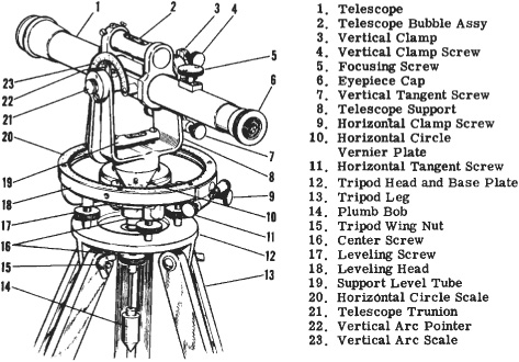
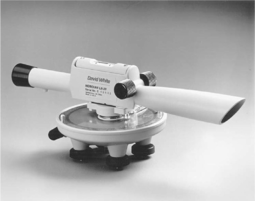
Builders’ Level. Figure 2.1 shows a type of builders’ level which is convenient for general contractors’ use. The telescope is held rigidly in a frame that rotates on a vertical spindle, which is perpendicular to the line of sight of the telescope. A spirit level with a graduated glass is mounted on the frame.
The leveling head on which the spindle rotates is fitted with a horizontal circle marked in degrees, in contact with a pointer fastened to the spindle. Many levels do not have this circle, but it is essential for the location work to be described.
FIGURE 2.1 Builders’ or contractors’ level. (Courtesy of David White, LLC.)
Vernier. The pointer may be expanded into a vernier such as shown in Fig. 2.2. This is a device for reading fractions of a scale, which in the example is calibrated to 30″ (half degree) divisions. The length of 29 divisions on the circle is divided into 30 divisions on the vernier. Each vernier space therefore represents  of a space on the circle and is
  shorter.
In the illustration, if an angle on the main scale is being read from left to right, the zero, or center of the vernier, shows a reading slightly higher than 2°30″. Reading the vernier to the right, it will be found that the tenth division line matches exactly with a line on the circle scale. This indicates that the zero mark was  , or one-third, of the way from 2½° mark to the 3° mark, as the difference is canceled out in the course of subtracting the difference 10 times.
One-third of 30″ is 10″. The angle is therefore 2°30″ plus 10″, or 2°40″.
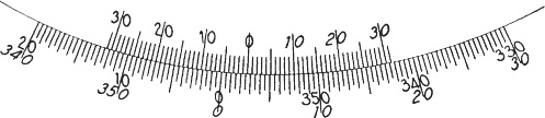
If the angle were being read from right to left, the main scale would read 357° and a fraction. Reading the vernier to the left, the twentieth division is found to correspond with a line on the circle. The angle is therefore 357° plus  of 30″, or 357°20″.
The telescope may be locked against swinging by means of a thumbscrew for convenience in reading the scale, or holding it in a certain direction. Another thumbscrew (tangent screw) will then move it slowly for fine adjustments.
Telescope. The length and power of the telescope and the length of the spirit level determine the range of the instrument and, to a considerable degree, its accuracy. Telescopes range from 10 to 18 inches (254 to 457 mm) in length, and from 10X to 35X power in magnification. Spirit levels may be 3 to 10 inches (76 to 254 mm) long.
The telescope is focused by means of a knob on the side or top, and possibly by a turning eyepiece also.
The field of view of the telescope is divided into quarters by the crosshairs, shown in Fig. 2.3(A), which are held in a frame or diaphragm inside the telescope. Provision is usually made to make these visible or invisible by focusing the eyepiece. The horizontal hair is used for taking levels. If it is correctly placed in the telescope, and the telescope is properly leveled, it indicates the slice of the field of view which is level with the observer’s eye. The vertical hair is used to sight a given point or line, and indicates the exact center of the field of view for determining horizontal angles.
Stadia Hairs. Stadia hairs (B) may be fitted into the same frame. These are horizontal and are located above and below the center hair. The distance between the stadia hairs is fixed at a ratio with the telescope, usually 1 to 100, so that if a measuring rod is sighted through the scope, the inches (millimeters) or feet (meters) seen between the stadia hairs may be multiplied by 100 to give the distance of the rod from the instrument.
Amateurs are apt to confuse one or the other stadia hair with the crosshair in taking levels, with resultant serious error. If this trouble persists, additional hairs may be installed, as in (C) in the form of a letter X, which should make the center hair easy to distinguish.
Base. The leveling head is mounted on the turntable or base by means of a center pin, on which it can both tip and rotate, and four leveling screws. These screws are threaded into the leveling head and rest on the leveling plate or turntable. They are expanded into knurled wheels for convenience in turning with the fingers, and have expanded feet which do not turn with the screw and which protect the plate.
The turntable base has internal threads by means of which it can be screwed on to the tripod head. It may have a hook on the bottom, at the center, from which a plumb bob (pointed-tip weight) may be hung by a chain and string. The base may be made to slide a limited distance horizontally, relative to the tripod head, for convenience in centering the unit directly over a mark.
Tripod. A tripod consists of three metal or wood legs, hinged together by a top plate which is threaded for the instrument, as seen in Fig. 2.4. These threads should be protected by a cap whenever the instrument is not mounted. The legs may be one piece, or two pieces sliding on each other and locked by a screw clamp.
The base may be set directly on a flat rock or stump, if it is not possible to set up the tripod, but this is not recommended.
Compass. Compasses are standard equipment in transits, and can usually be obtained for other types of instruments that have a horizontal scale. They are not necessary for the work to be described in this chapter, although it is often convenient to know the general directions of lines.

FIGURE 2.3 Sighting hairs. (Courtesy of David White, LLC.)
FIGURE 2.4 Parts of level transit. (Courtesy of David White, LLC.)
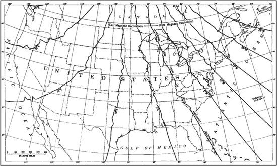
Surveys are generally based on the true north, from which the compass north varies rather widely. Part of this variation may be obtained approximately from the map, Fig. 2.5, or exactly from local sources.
If you are in an area of west magnetic declination, the compass needle will point west of the true north by the amount shown on the map.
Another source of error is the magnetic attraction of magnets, iron, and iron ore for the compass needle. It is also affected by the time of day. No confidence should be placed in a compass reading taken near machinery or electrical apparatus. Metal objects in the observer’s pockets may cause errors.
Setting Up. The first step in using the instrument is to set up the tripod. The top should be as level as possible, and the legs pushed into the ground firmly. On a slope, two legs should be downhill. The protecting cap is removed and the instrument screwed on. The telescope frame should be unlocked so that it is free to rotate. The telescope can then be held in one hand and the base screwed on the tripod with the other.
Leveling. The instrument must now be leveled by means of the four screws. The telescope is turned so that it is over two of them, and those screws are adjusted until the bubble in the level is exactly in the center of the scale. The screws are turned at the same time in opposite directions, so that one pushes the leveling head up while the other makes space for it to come down, as it pivots on its center pin.
The bubble moves in the same direction as the left thumb, as indicated in Fig. 2.6A. If the two screws are turned exactly the same amount, the tension on them will remain constant. If the screw toward which the bubble is moving is turned farther, it will jam both screws. If the screw behind the bubble is turned the most, the tension will be reduced and the screws may lose contact with the turntable.
FIGURE 2.5 Magnetic declination map. (Courtesy of U.S. Coast and Geodetic Survey.)
If both screws are turned to the left (clockwise), or one is turned left while the other is stationary, they will be jammed; while if one or both are turned to the right (counterclockwise), they will both lose contact.
The screws should be kept in light contact with the plate during the adjustment and tightened somewhat as it is finished.
When the bubble is approximately centered, the telescope should be swung 90 degrees so as to be over the other pair of screws, which are used to center the bubble in the same manner. This adjustment will disturb the first one, so the telescope must be swung into its original position and leveled, this time more exactly. It should then be checked in the second position, and adjustment in the two positions made alternately until it does not move during the swing through this quarter-circle arc.
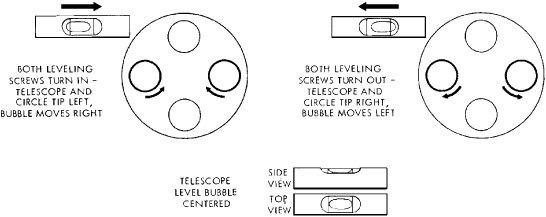
FIGURE 2.6A Leveling screw action. (Courtesy of David White, LLC.)
The telescope should now be swung through the other three-quarters of the circle. If the adjusting screws are tight and the tripod has not been disturbed, the bubble should not move. If it does move, and the table cannot be leveled so that it will not move when swung, the spirit level is probably out of adjustment.
Releveling. During use, the spirit level should be checked occasionally and the instrument releveled if necessary. The tripod may settle into the ground, particularly if on some unstable base such as ice, wet clay, or oil road top. Jars from focusing the telescope, or the wind, or other causes, may disturb it. Sometimes it is necessary to put small boards under the legs to avoid settling.
Centering. Exact placement of the instrument is usually not important in setting grades, but it is essential in most other work. It involves locating the vertical axis on which the telescope swings directly over a marker, often a nail in a 2×2 inches (51×51 mm) stake.
The standard procedure is to hang a pointed, balanced weight called a plumb bob from the center of the instrument by a light chain and/or string. The tripod is maneuvered until the point of the bob is just over the center of the nail head.
This location may need readjustment after leveling the instrument, and such relocation calls for releveling.
The tripod head in Fig. 2.6B allows horizontal shifting a distance of 2 inches (51 mm) in any direction, without disturbing its level. This device saves time and trouble.
The optical plummet, Fig. 2.7, replaces the plumb bob with a low-magnification telescope in the rotating base, which, by means of a prism, looks down the vertical axis. A small bull’s-eye and cross line make possible exact alignment with a marker.
Transit Theodolite. A transit has a vertical swivel and support yoke mounted on the turntable, which permits the telescope to be tilted up and down on a vertical axis in addition to its horizontal rotation. The angle from the horizontal is shown on a vertical scale with a vernier. When it is used as a level, the reading on that scale should be zero.

FIGURE 2.6B Shiftable tripod head.
A level transit like the one shown in Fig. 2.4 can be tilted in the vertical plane 45 degrees, either up or down. Full transits have an extended support yoke that permits the telescope to turn in a full vertical circle within it. This makes it possible to make a back sight (180° turn) without changing the setting of the horizontal circle.
The latest transit theodolite is computerized for easy, quicker setup and readings. Figure 2.8 shows one of these electronic theodolites for routine layout and measurements on a building site. The compact instrument offers user guidance through the measuring processes and programs. There are only seven keys used for control of the straight forward and fast operation. On the press of a key, both the computed and measured data appear in a clear four-line display. In the measuring programs, the user guidance is supported by a graphical display, making the solution of the problem easier to follow and accept or correct.
The self-leveling or automatic level uses a three-screw leveling base with a circular level vial, for approximate leveling of the instrument. Fine leveling is done by a gravity-controlled device (pendulum or compensator) inside the telescope. See Figs. 2.9A, 2.9B, and 2.9C.
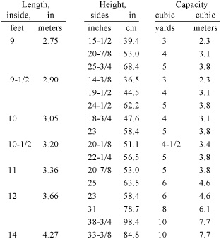
The surveying instrument’s best companion piece is the leveling or target rod. This is a measuring stick, marked in feet, tenths of feet, and hundredths of feet; or in feet, inches, and eighths of inches. It may be 8 to 15 feet (2.4 to 4.6 m) long, and usually is in two or three pieces which slide on each other, or, occasionally, are hinged or pegged together. The sliding type must be fully closed or fully open to be accurate.
Long rods are very desirable in hilly country.
Spaces may be marked by fine lines similar to those on a ruler, in which case it is called a New York rod. A Philadelphia rod uses the division lines as units of measurement in themselves. See
FIGURE 2.8 Electronic theodolite. (Courtesy of Carl Zeiss, Inc.)
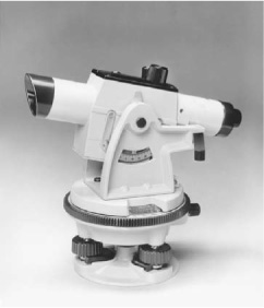
FIGURE 2.9A Automatic level transit. (Courtesy of David White, LLC.)
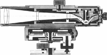
FIGURE 2.9B Cross section of self-leveling level. (Courtesy of Carl Zeiss, Inc.)
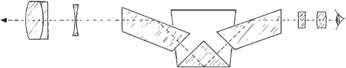
FIGURE 2.9C Line of sight in self-leveling level.
Fig. 2.10A. A rod in the decimal scale has the tenths of feet each divided into 10 equal sections, alternating black and white. If inches (millimeters) are shown, each is divided into eight equal bars of alternating color.
The target, Fig. 2.10B, is a metal disc that slides on a track on the sides of the rod. It is painted in quadrants, alternately red and white, with the division lines horizontal and vertical, or in other conspicuous patterns.
The rod operator moves the target up and down on the rod in response to signals from the instrument operator. Readings can be taken in this way when distance or haze prevents reading of figures on the rod.
The target may include a vernier, in which case it can be used for precise work requiring reading of fractions of the smallest divisions of the rod scale.
The rod is used for measuring the distance from the instrument’s line of sight down to a point. If the point is almost as high as the instrument, this distance will be short; if it is much lower, the distance will be long.
The elevation of a point is the distance which it is above some standard level. This may be mean sea level—halfway between high and low tide marks—or some local point to which an elevation is assigned arbitrarily.
Elevations are usually positive numbers, measured up from a base point or plane. Rod readings are negative, being measured down from the plane of the instrument.
In taking levels, the positive elevations are obtained from negative rod readings. Care must be taken to avoid confusion. It must be remembered that for any instrument setting, the high readings are low elevations, and vice versa.
FIGURE 2.10A Philadelphia rods.
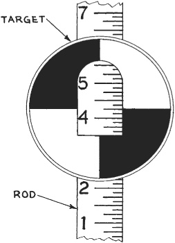
FIGURE 2.10B New York rod and target.
Use of the instrument as a level depends upon the fact that its crosshair indicates a horizontal plane, level with the observer’s eye in all directions. By use of the rod, the amount by which a point is lower than this plane can be measured, and the relative elevation of any number of points within range can be calculated from rod readings. Points above the crosshair cannot be measured, except on vertical walls, without moving the instrument higher and resetting it.
Levels are most accurate over short distances. If the instrument must be used when out of adjustment, readings should be taken as nearly as possible at equal distances.
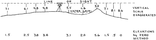
Converting Readings to Elevations. If the instrument is to be set up only once on a job, and no record is to be made of observations, the rod readings can be used to figure heights. However, since these numbers are negative, the beginner will avoid confusion by calling the lowest point—that with the highest rod reading—zero elevation. The other points will then each have an elevation equal to the difference between its reading and that of the zero point. See Fig. 2.11.
Benchmarks. If the elevations are to be recorded for future use, it is necessary to have some fixed reference point which will not be disturbed and which can be readily identified. A knob on firm bedrock, a nail projecting from a tree trunk, a mark on a building, or a stake hammered flush with the ground may be used. Such a point is called a benchmark, and is abbreviated as BM. A reading is taken the first time the instrument is used, and again each time it is set up. These readings will probably all be different, but in each case the elevation of the instrument may be found by adding the rod reading when the rod is sitting on the benchmark to the benchmark elevation.
Since the benchmark is the most permanent point observed, it is good practice to assign an elevation to it, and to calculate all other elevations from that. An assigned number should be large enough that no elevation less than zero will be found on the job, as working with minus figures may cause confusion and error.
If levels have been taken previously in the area, engineers’ benchmarks may be found, in which case it is wise to use them. If possible, the elevation assigned to them in the previous survey should be used to facilitate comparison between the two sets of levels.
Even if engineers’ benchmarks cannot be used directly in surveying the job, it may be advantageous to run a level to one, and note its elevation in relation to the contractor’s own benchmark, so that the two systems can be compared if necessary.
If the job is a type that will involve frequent checks of levels, as on a road where stakes may be knocked out by machinery, it is a good plan to set up benchmarks so that one will be visible from each point where the instrument will be used. This saves time in taking grades on a few stakes and eliminates common errors in moving the instrument, or in taking an elevation from the wrong line stake, or a stake which has been disturbed.
All benchmarks should be figured very carefully and rechecked at least once.
Recording Readings. Another requirement in recording observations is to identify the spot at which each reading is taken. This is usually done by taking readings at set intervals, such as 10, 50, or 100 feet (3, 15 or 30 m). These distances should be marked by stakes, pegs, small rock cairns, or in other ways. The first stake or mark of the series is called the zero stake, and the others are identified by their distances from it. It is customary to give distances in units of hundreds, followed by a plus sign and the other figures of the distance. The zero is written 0 + 0, the 50-foot (15-m) mark 0 + 50 (0 + 15), and the 100-foot mark as 1 + 0. If any points on the line are needed which are not in the series, the distance is measured and entered in the notes with the reading, as 0 + 35 feet (0 + 10.7 m).
Important ground features along the centerline, such as crests of rises, bottoms of dips, or beginnings of rock outcrops, should be taken in addition to the stake readings.
Elevations may be taken from the ground, from the top of the stake, or more rarely, from a mark on a stake. If taken from the ground, it should be stamped or cut flat. Such readings are not as accurate as those taken from the top of a stake, and may be very difficult to check back, but they can be used directly in preparing profiles and figuring cut and fill. If the top of the stake is used, it is necessary to measure the stake height.
Tapes. Measuring is usually done with a steel tape, often called a chain by surveyors. Fifty-foot (15-m) and 100-foot (30-m) lengths are standard, and will suffice for most purposes. They should have a nonrusting finish, as it is often difficult to dry and oil them immediately after wet work. Care should be taken not to kink a tape, or to bend it sharply, as such abuse may break it.
If the numbers become illegible, they can be fixed for rough work by measuring and marking the feet, and perhaps some fine divisions, with paint. A broken tape can be repaired by means of a splint and two rivets.
Cloth tapes stretch readily, and are not accurate enough for even rough use. Metallic tapes, composed of cloth with interwoven wires, are variable in quality and resistance to stretching. If used, they should be checked occasionally by a good steel tape.
Steel tapes change length with temperature and stretch under tension, but these changes are so small that they can be ignored in open work.
Tapes must be held level, or very nearly so, on slopes, as engineers’ land measurements refer to distances on a horizontal plane. The downhill end of the tape may be placed exactly above the desired point by use of a plumb bob, or by dropping pebbles from the tape end.
Centerlines usually include angles or curves. If the former, measurements must be made to and from the angle point, rather than by a shortcut. Gradual curves may be measured in a series of chords (straight lines beginning and ending in the curve). Sharper curves may require a reduction in the length of the chords, as from 100 to 50, 25, or even 10 feet (30 to 15, 7.5, or even 3 m). The difference in length between the chord and the arc of the curve may be readily found by laying the tape along the curve from one chord point to another; or measuring a distance along it in very short chords, then measuring the distance between the two points directly. If no significant difference is found, the chords are not too long.
Tapes are best suited to two-person use. However, the loop on the zero end can be anchored in dirt with a screwdriver, and to stakes with a pushpin or thumbtack, and measurements made by one person.
Ground measurements may also be made with the rod, with a short rule, a stick of known length, or for very rough work, by pacing.
Stadia. If the instrument is equipped with stadia hairs, it may be used to measure distance as well as elevation. If the stadia ratio is the usual 1 to 100, and the rod is marked in feet, tenths and hundredths of feet (meters), each tenth visible between the stadia hairs indicates a distance of 10 feet (3 m) from the center of the telescope to the rod. Six tenths would mean a distance of 60 feet (18 m), a foot would mean 100 feet. This distance may be noted at the same time as the crosshair reading.
If the rod is marked in feet, inches, and eighths of inches, each inch indicates a distance of 8⅓ feet (2.5 m), each foot 100 feet (30 m).
If a distance is to be measured off, the rod is held at increasing distances from the instrument in response to signals, until the proper number of markings shows between the stadia hairs.
The rod should be held perpendicular to the line of sight. The correct angle can be found by pivoting it slowly toward and away from the instrument, until the minimum reading is obtained.
Turning Points. If elevations are to be taken for any points above the crosshair, the instrument must be picked up and reset at a higher elevation. It must be located so that it can take a reading on at least one point that was taken from the old setting. This point (turning or transfer point) is preferably one of the higher elevations (low readings) taken, and should lie between the two instrument locations. It is best taken from the top of a firm stake, or a knob or a well-marked spot on rock or hard ground, so that the rod set on it will be at exactly the same height at the second reading as at the first. Accuracy in reading at the turning point is very important, as any error made will persist through the rest of the survey. Amateurs are advised to use two turning points with each move, as mistakes in reading or in arithmetic should then show up immediately.
The new instrument elevation (abbreviated H.I. for height of instrument) is found by subtracting the smaller reading from the larger one for each turning point, and, in an uphill move, adding the result to the first elevation of the instrument.
Recording and Figuring. Figure 2.12 shows some of this work. Part (A) shows the slope, the location of benchmarks and stakes, and the two instrument positions used. Part (B) is an informal set of notes of rod readings and calculated elevations. Part (C) is a profile drawn on cross-section paper from the notes in (B). It is made by drawing a baseline, assigning it an elevation lower than those of the stakes, and making each square represent a certain distance. In this diagram, each square represents 1 foot (0.3 m) vertically and 10 feet (3 m) horizontally. This vertical exaggeration is necessary to have a large enough scale without making the drawing impossibly long.
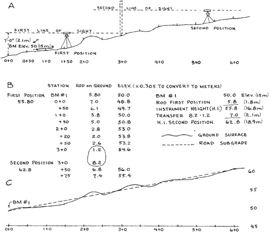
FIGURE 2.12 Recording and figuring. (All measurements given in feet.)
The profile is useful in giving a picture of the slope, in determining gradients of roads or ditches, and in figuring the cut and fill necessary to convert the present grade to the new one.
The dotted line is the subgrade for a proposed road. It will be seen that the depth of cut or fill on this line may be approximately determined by measurement with a ruler; the elevation of any point on the road, in relation to the benchmark, can be found in the same manner.
Moving Downhill. If, at the original or at any later location of the instrument, points to be taken are so low that the rod is below the crosshair, the instrument must be moved downhill. A turning point (or points) is chosen with the lowest possible elevation (highest reading), the instrument is moved, and new readings are taken. The low reading is subtracted from the high one, and the result is subtracted from the earlier instrument elevation.
If only one or two points slightly below the crosshair must be taken, the rod may be set on a stake, and the height of the stake added to the reading; or a ruler may be used at either the top or the bottom of the rod to extend it.
Check Runs. When all the necessary points have been taken, the accuracy of the work may be checked by taking levels back to the starting point. This is usually a faster operation than the outward trip, as it is only necessary to take transfer points and benchmarks. If frequent benchmarks have not been placed, it is advisable to use the same turning points, or to take readings on a few of the grade points, so that if an error is present, it may be localized. It is not necessary or desirable to set up the instrument on the same points for the return trip.
The two elevations found for each point should agree, but a difference, varying with the care with which the work is done, generally exists. Benchmark runs should be held to within a few hundredths of a foot, even in rough work where a difference of several inches on a grade point might be allowable. If any considerable amount of cut or fill is needed, even benchmarks may be left as approximations, until skill or time is available for a more careful run. Any discrepancies found in the check run should be listed in the notes.
If benchmarks are set at the beginning and end of a run, and check properly on the return trip, it will not be necessary to back-check any later run on which these two elevations show correctly. However, if benchmarks have been set by other parties in some previous survey, they should be checked the first time they are used, as they may be wrong or their description misunderstood.
Grade Stakes. Centerline road stakes are set by instrument and measurements from a prepared baseline. Shoulder, slope, and other side stakes are set from the centerline.
Grading information, that is, the cut or fill necessary at each stake, may be determined in several ways. The preferred method is to take the ground-level elevation at each stake by instrument and rod to the nearest hundredth of a foot (meter) or eighth of an inch (millimeter), figure the difference from the desired elevation, and mark the difference on the stake.
Ground is often so rough that some dirt has to be patted down flat at the foot of the stake to provide a recognizable base for the rod. It may be advisable to put a crayon mark on the stake at ground level, in case anything should change it. This mark, usually a horizontal line, will be needed when grades are marked on it.
Many surveyors prefer to use the top of the stake rather than the ground level. In this way they have a firm base for the rod, and they do not have to be concerned with the possibility that dirt might be kicked away or added. However, this usually requires measuring the stake height to give ground level for yardage calculations.
A horizontal crayon line on the stake may be used instead of the top or ground.
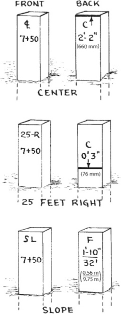
The elevations observed at the stakes are subtracted from those required by the road plans. Plus numbers indicate that fill is needed; minus numbers that the ground must be cut or removed. The symbols written on the stakes are F for fill and C for cut. Each stake must show location.
Another method is to supply the surveying crew with the required grade elevation for each stake. These are subtracted from the H.I. (height of instrument) to show the reading on a rod held with its bottom at correct grade at that location.
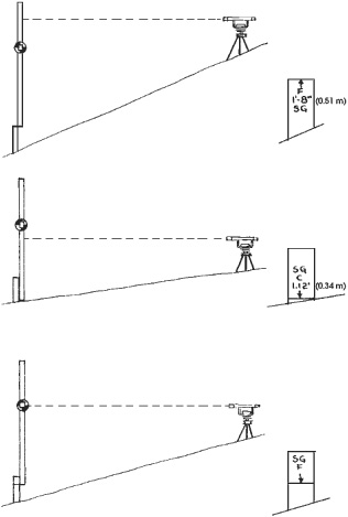
If the rod can be held at an elevation so that the reading is seen at the instrument crosshair, the stake is marked with a horizontal line at the base of the rod. This line is marked SG or G. The indication is that ground level must be raised to this line.
If the top of the stake is below the grade, the rod is placed on its top. The calculated reading is subtracted from the actual reading, and the difference written on the stake, following the symbol F. A crayon line is made at the top of the stake, and/or an arrow is drawn from the figures to the top. See Fig. 2.13A.
Such a measurement for fill can also be made from a line drawn at any convenient height on the stake. It might be positioned an even distance below the grade, as 2 feet (0.6 m).
If the rod shows less than the calculated reading when it is resting on the ground, a cut is indicated. A line is put on the stake at ground level, or at some other convenient height, and a reading is taken of the elevation of the line. The actual reading is subtracted from the calculated reading, and the difference written on the stake, following the symbol C, as shown in Fig. 2.13B.
Stakes placed for the guidance of earth-moving crews should indicate cuts and fills to the grade they are working to produce. This is usually a subgrade, symbol SG, that is lower than the pavement surface or theoretical grade, G. It is very important to make clear which elevation is meant.
Road stakes are discussed in Chapter. 8.
Engineers’ grades usually consist of a series of elevations for the finished road. These are plotted on the same sheet of cross-section paper as the profile of the ground surface, and the depth of cut or fill is determined by measuring the distance between the two lines. These figures, if used directly, will not be accurate for most subgrade work, as the thickness of the pavement or gravel and of any special subgrade material must be subtracted to obtain the rough grade elevations.
A misunderstanding as to whether figures on grade stakes are for finish grade or subgrade can be very expensive. Use of subgrade figures for preparing subgrades is usually most satisfactory.
The contractor may obtain from the engineer a list or profile showing subgrade elevation at each station, and information as to the location and elevation of benchmarks. This, combined with sufficient field references to show the centerline, will enable the contractor to replace stakes which have been knocked out, and to find the depth of cut or fill required, by comparing the ground elevation with that required for the road.
Turning Angles. When an instrument is used to turn angles—that is, to measure the horizontal angle between two lines or directions—the axis of revolution of the telescope must be exactly above the intersection of the lines, which may be marked by a nail in a stake driven flush with the ground, a cross chiseled in rock, or markings on concrete or metal plugs.
When the instrument is set over a point, a plumb bob should be hung at its center of rotation from a hook or through a hole usually provided. The point of the plumb bob should be just above the mark, and an amateur may have to move the tripod repeatedly before it is placed right.
If the instrument has a shifting base so that it can slide on the tripod, setting up over a point is greatly simplified.
A range pole is a convenient accessory in line and angle work. It is a pole 7 or 8 feet (2.1 or 2.4 m) long, equipped with a metal point. It is painted alternately red and white in bands 1 foot (0.3 m) wide. It is lighter than a rod and because of its conspicuous pattern is more readily seen at a distance.
This pole is set on one of the lines in question. The instrument is swung so that the vertical crosshair is on the pole. The rotation is locked, and the hair lined exactly on the pole by turning the horizontal tangent screw.
The reading on the horizontal circle and on the vernier is recorded.
The pole is placed on the other line and sighted in the same way. The difference between the two readings is the angle between the lines.
Line and angle work may be done to stake out on the ground locations described on a blueprint or map; or to make a record of ground features or locations on paper so that they may be used in figuring, or replaced or relocated if necessary.
Staking out is best left to surveyors if possible, as accurate work involves trigonometry and skillful use of the instrument, and inaccurate work may result in very expensive mistakes. However, in emergency, or when results need be only approximate, contractors can do it themselves.
Recording. If the location of existing stakes is to be recorded so that they can be replaced if destroyed. The work is the same except that the angles are obtained by sighting the instrument and coping from the horizontal circle onto a sketch. Distances are measured in the field and noted on the sketch, which is most conveniently made on cross-section paper, roughly to scale. This sketch is used in the same manner as the map in the previous discussion in replacing the stakes. Results are generally much better, as the field figures are more accurate than those obtained with ruler and protractor from the map.
If field observations are to be entered on a map, the baseline or points should be related to features shown on the map, as corner stakes, points measured on a line between diagonal corners, or measured along a boundary. When the baseline is correctly drawn, angles and distances can be marked in with protractor and ruler.
Without Instruments. Simple location work can also be done without instruments. Figure 2.14 shows a square building plot. Lines are drawn on the print or tracing prolonging each side of the house to the plot boundaries, from where the distance to the corners is measured. These distances are then measured off on the ground, and stakes are set.
The distances of the house corners from the boundary lines may be scaled from the map and measured on the ground in directions found by sighting between pairs of boundary stakes.
Sighting may be done by placing a thin straight stake, as at L, and another at Q.
A person may stand behind the stake at L in such a position that, when she or he looks with one eye, the stake at Q is centered on L and just above it, as in Fig. 2.14(B). Another person, carrying a third stake, measures the distance QE, keeping on line LQ in response to directions from the observer. The measuring is best done by pinning the tape to Q. The stake is set at E so as to be directly in line between stakes L and Q. The distance EC is then measured, and stake C set in the same way. Distance CL is measured for a check.
Stakes F and D may be placed according to sighting from M to P, and measurements similar to the method used for E and C. The four corners of the building are thus located, and in a regular plot such as this no more work would be needed.
However, as a precaution against error, or in an irregular plot, or one with poorly defined boundaries, it is wise to prolong the other sides of the house into lines JO and KN, and to sight and measure the corners again from J and K.
Reference Stakes. If the corner stakes have been set for a building in a plot without definite boundaries, and the contractor wishes to be able to reset them if necessary, there are several ways in which markers can be set without instruments.
In Fig. 2.15 the house wall lines are shown continued in straight lines out of the digging area. These lines may be established by putting sighting poles on the corner stakes and finding a distant position from which two of these are in line—that is, one partly or completely hides the other. This sighting should be done with one eye and a pole held vertically in line with them. A stake is driven to mark the position of this third pole. The distance from this to the nearest corner stake is measured. This process is repeated for each pair of stakes at the foundation. In the figure, the reference stakes are indicated by Xs and the sight lines by dotted lines. A sketch should be made showing distances.
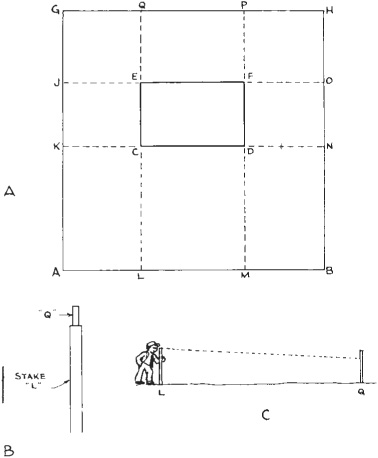
FIGURE 2.14 Staking without instruments.
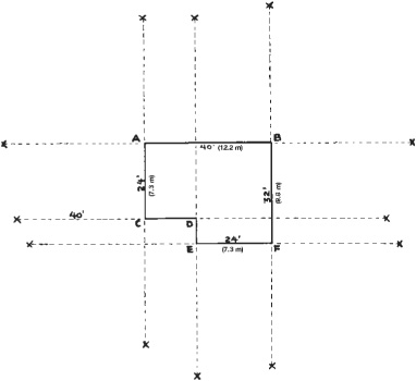
FIGURE 2.15 Cross-reference stakes.
Any missing stake may be found by sighting from one marker to the other one on the same sight line, and measuring from the nearest marker. Even if the sketch is not available, the point may be found by the intersection of two lines of sight, as described under instrument work.
If each reference stake is set the same distance out from the nearest stake, there is less need of keeping a record.
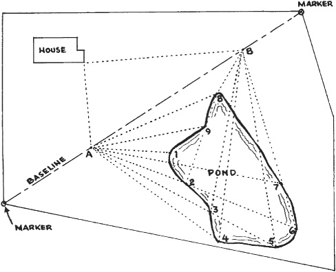
Locating a Pond. If an irregular shape, such as a pond, is to be roughly measured and drawn into an existing map, a baseline is first established and two points are measured off. A number of pegs are driven into the shores of the pond at points which will serve to indicate its outline, and are numbered in rotation, as in Fig. 2.16. An instrument with stadia hairs is set up at A, a sight taken on B, or on a more distant marker along the baseline. A sight may also be taken on a corner of the house for a check. Sights are taken on all the stakes in rotation, starting at one, the angle read for each one, and the stadia distance recorded. This information is sufficient to locate the pond by drawing the baseline on the map, and plotting distances and angles. However, to avoid the possibility of gross error, it is safer to set up at B, take a bearing on A, and record the angle and distance of some or all of the points observed from A.
The area of a pond so plotted can be easily obtained by counting squares on cross-section paper, or by the use of a planimeter, which is a small instrument used for measuring areas on paper.
Grids. If it is necessary to map an area, locating buildings, drainageways, trees, or other features, or to take elevations over a large area in order to prepare grading or drainage plans, a grid should be laid out. This consists of pegs or stakes at set intervals. They should be in straight lines, crossing each other at right angles. These lines, intersecting at the pegs, generally divide the area into squares. The interval may be 5 to 20 feet (1.5 to 6.1 m) or more.
FIGURE 2.16 Locating by stadia.
The grid may be laid out in a number of ways. A baseline should be laid out along an edge of the area. The instrument, preferably a transit, is set up at a corner of the proposed grid and sighted along the baseline. Pegs are set every 10 feet (3 m), or at any other desired interval, measured from the instrument, to the end of the grid. Tape measurement is preferable.
The instrument is now turned 90°, and pegs are set at the same interval along the line of sight to the end of the grid. The instrument is set up at the end, a backsight taken, and a 90° turn made. Pegs are set at the same intervals along this third line.
The interior pegs may be placed by the use of a long tape from opposite pegs, or the instrument may be set up over each peg in either the first or third lines, sighted at the corresponding peg in the other line, and pegs set according to its vertical hair and measurement.
Obstacles may make it possible to set all the pegs by any of these systems. Usually, if as many pegs as possible are placed, the rest can be filled in by sighting along lines of pegs, with reasonable accuracy.
The grid should now be copied on cross-section paper with a point representing each peg. Any landscape features may be readily sketched in by estimating or measuring the distance from the nearest peg, and noting the place of the peg in the grid.
Elevations are now taken on each peg, preferably doing them a complete line at a time to avoid confusion. The rod reading may be written just above each point. Readings should also be taken on high and low spots, drain channels, and anything else of interest, and noted in the correct place on the paper.
When the instrument work is finished, the readings are preferably converted to positive numbers that can be penciled below the points, and the rod reading is crossed out.
This grid sheet can be used for reference for any locations or grading estimates which may be required, and in drawing contours, profiles, and cross sections.
Grids without Instruments. If no instrument that will turn angles is available, a grid may be laid out with a tape, and elevations taken with a hand level. A baseline is decided upon, and a tall stake set at each end. A tape—the longer, the better—is pinned at one end and extended toward the other, and lined up by sighting across it from one stake to another. The intervals are measured, and the tape is moved on and lined up again.
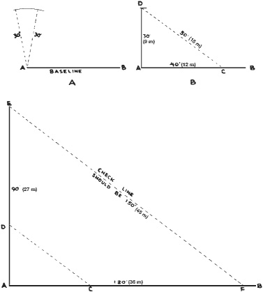
The right angle may be laid out by referring to the ancient engineering knowledge that if the sides of a triangle are in the proportion of 3 to 4 to 5, the angle between sides 3 and 4 is a right angle. The process is illustrated in Fig. 2.17.
First the baseline is laid out, measured off, and pegs are set. The tape is pinned at A, one end of the baseline, and 30 feet (9.1 m) is measured off at approximately a right angle. The tape is moved back and forth in an arc that is marked on the ground.
The tape is then pinned to the baseline at C, 40 feet (12 m) from the end, and an arc of 50-foot (15-m) radius described, crossing the first arc. A stake is driven at the point where these arcs intersect. Line AE may be located by sighting along stakes A and D, and will be perpendicular to AB.
These figures have been given for the use of a 50-foot tape, but any measurements may be used as long as the 3:4:5 relationship is preserved. Larger triangles will give greater accuracy. If the grid is large in proportion to the triangle, a diagonal should be measured from E to a point on the baseline either ¾ or 1⅓ as far from A as the distance AE, and any necessary correction made if the diagonal is not in the proper proportion.
A very rough grid may be made by sighting along the sides of a building to obtain the right angles, and spotting in the pegs by eye and measurement.
Obstructions. Buildings, vegetation, and rough ground interfere seriously with primitive instrument techniques and make it more economical to hire an engineer.
Large permanent obstructions require layout of additional lines and angles to work around them.
Brush clearing for sight lines is laborious and sometimes quite destructive. It is handled by setting up the instrument, pointing it in the desired direction, and directing the cutters so that their work will be kept close to the line of sight.
In heavy undergrowth a mistake in turning an angle may waste hours of cutting work.
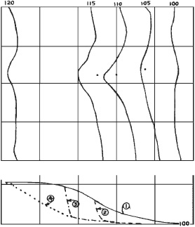
Contour Lines. A grid is frequently used to make a contour or topographic map of an area, as in Fig. 2.18.
A contour line is a line joining points of equal elevation on a surface, or the representation of such a line on a map. In mapping, contours are drawn at set intervals whose size depends on the roughness of the ground and the scale of the map. In nearly flat areas contour interval may be 1 foot, while in steep mountains 100-foot (30-m) intervals are usual. Every fifth line is drawn more heavily than the others, and its elevation is printed in it.
A contour interval of 2 feet (0.6 m) is used in the illustration. The profile shown below the map is plotted along the dotted line. Note that grid points alone would not have shown the depression crossing it.
Since few of the grid points are exactly at a contour elevation, it is necessary to estimate the lo cations of the lines as they pass between higher and lower points, a process that is called interpolation. The 88 contour is placed halfway between point A-3, elevation 87.4, and B-3, elevation 88.6, as it is the same distance above one as it is below the other. The same line passes between B-1 and B-2, elevations 84.1 and 88.1, respectively. In this case the 88 contour is placed very close to B-2.
In irregular land it is very important that the grid observations include the crests of ridges and the bottoms of gullies, as the contours cannot give an accurate picture of the ground if they are omitted. The grid interval must also be close enough to show all important ground features.
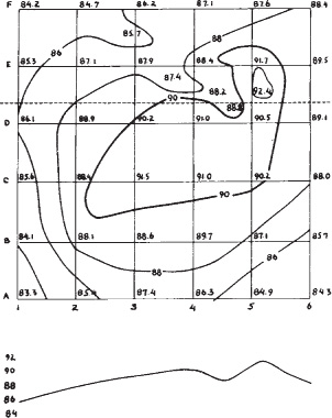
Placing of contours therefore cannot be an entirely mechanical operation. In the first place, the person making the field notes must understand topography sufficiently to take extra readings where necessary to show up special forms. The valley at the top of this map would not have been shown at all by readings on the grid points only.
The person drawing the contours should have a feeling for landscape forms, to avoid misinterpreting the data from which she or he works.
Topographic Map. A topographic map is usually a contour map on which both natural and artificial features are indicated. The U.S. Geological Survey, Washington, D.C., has small-scale maps covering most areas of the country that show contours, vegetation, roads, trails, lakes, streams, and much other information. These maps are sold by mail and in bookstores at nominal prices. They are handy for many purposes and essential for some jobs.
Profiles and cross sections may be taken from a contour map by laying a ruler across it, measuring the interval between contour lines, and posting distances and elevations to cross-section paper. The proposed new grades can then be drawn in, and the differences calculated.
The topographic map has a wide variety of uses, including locating highways, haul roads, borrow pits, and dump areas; studies of drainage and stream flow; and estimation of quantities in cuts and fills.
Surveying instruments are delicate and are easily put out of adjustment by failure of parts, careless handling, or accidents. It is often not possible to have them checked or repaired locally; the return to the factory may mean loss of use for weeks or months.
It is therefore desirable that a person using an instrument be familiar with some adjustments that can be made in the field, without special skill. These include setting of telescope spirit level, and the horizontal and vertical crosshairs.
If these are properly set and the instrument is inaccurate, shop service is probably necessary.
Spirit Level. The telescope spirit level is usually fastened by a pair of vertical bolts. A single nut holds it in a fixed position at one end, and a pair of nuts, one above and one below, permit moving it up and down on the other end.
This level can be checked each time the instrument is set up. When the turntable is level, the telescope should be able to swing in a full circle without changing the position of the bubble. If no turntable screw adjustment will permit this, the level is presumed to be at fault.
To adjust, the turntable is leveled as accurately as possible and the bubble centered. The telescope is swung a half circle, causing the bubble to shift. The bubble is brought one-quarter of the way back to center by the adjusting nuts, and the rest of the way by using the turntable leveling screws.
The telescope is then swung to its original position, the bubble moved one-quarter of the way to center by adjustment, and centered by the leveling screws. This process is repeated until swinging the telescope does not affect the bubble.
Crosshair. If the horizontal crosshair is not exactly centered, all readings on the rod will be too high or too low. Readings taken at about equal distances will agree. Greatest errors will be found on long sights.
A reasonably accurate check and adjustment of this hair can be made with the help of a still pond. Two stakes are driven flush with the water surface, about 100 feet (30 m) apart. The instrument is set in line with them, 10 feet (3 m) beyond one.
A rod is set on the near stake and a reading taken. This is assumed to be accurate, because the distance is too short for a perceptible error. The target is locked to the rod at this reading, or a note made of it.
The rod is set on the far stake. If the hair is correctly adjusted, the reading should be the same. If it is not, the hair should be raised or lowered until it agrees.
This is done by turning setscrews at the top and bottom of the frame which hold the hair. The screws are unlocked by twisting one or the other a quarter or half turn, after which both are turned in the same direction.
If no pond is available, or a more accurate adjustment is required, two stakes should be driven firmly into the ground, 200 to 400 feet (61 to 122 m) apart, and at almost the same level. The instrument is set up halfway between them, as in Fig. 2.19(A), and leveled carefully.
A leveling rod is held on each of the outer stakes, and an exact reading taken according to the crosshair. These readings will be accurate with reference to each other, as any error in crosshair height is canceled in observations taken at equal distance.
The stake standing on lower ground is assigned an elevation of zero, and has the higher rod reading. The elevation of stake (b) is the difference between the two readings.
The instrument is now set up in line with the two stakes as in (B), about 10 feet (3 m) beyond stake (b). A reading is taken of (b). Then a reading is taken at (a), which should equal the elevation of stake (b) plus the reading there.
If it does not, adjustment is made in the manner described above.
Vertical Hair. The vertical cross or direction hair may be checked by driving three stakes exactly in line at 200-foot (61-m) intervals. The line may be determined by sighting with the vertical hair, and the distances measured by stadia or tape. The stakes should be about on the same level.
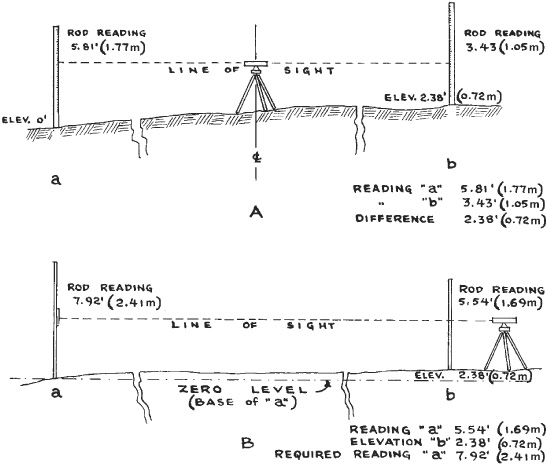
FIGURE 2.19 Checking the crosshair.
The instrument is set up over the center stake, leveled carefully, and turned so that the hair lines up with a rod or pole held vertically over one of the end stakes. The instrument is turned exactly 180°, or, if it is a transit, flipped over vertically. The hair should now line up with a vertical stick on the other stake.
If it does not, the crosshair should be moved one-quarter of the way toward the stick by means of adjustment screws on the sides of the crosshair frame. These work in the same manner as the upper and lower screws.
After the one-quarter adjustment, the telescope is turned until hair and stick coincide. A 180° angle is again measured off and the rod on the first stake sighted. The hair is adjusted to move toward it one-quarter of any distance, then centered on it by moving the scope.
Additional half-circle turns, and adjustments, are made until the hair will coincide with both sticks, 180° apart.
The word “laser” stands for “light amplification by stimulated emission of radiation”. The type originally used in construction was a tube filled with a mixture of helium and neon gases, stimulated by electric current.
Stimulation causes the gas atoms to emit energy in the form of light. This process produces light with only one frequency, with such intensity that it emerges as a continuous, coherent, narrow beam of red light. Its sides remain almost parallel for considerable distances, instead of diverging and widening as ordinary light.
In recent times the most common lasers used in construction are diodes. A diode is a two-electrode device having an anode and a cathode with marked unidirectional characteristics. This type of laser is an electron-wave tube, which derives its characteristics from the interaction of electrons which are in a beam of initially uniform charged density. The electron wave is focused in a narrow beam of high intensity. It may be in the visible light or infrared (IR) light range. Most commonly used in construction are red or, with certain filters, green which is more intense than the red light.
The IR lasers are used for heavy construction equipment in the short to medium range of 500 to 1000-foot (150- to 300-meter) radius from the laser. There is a laser receiver mounted on the excavator, backhoe, and the like, for elevation indication. With a slope control laser the beam can produce a high-powered IR or barely visible beam for a projection of 1500 or 2500 feet (457 or 762 meters), or more.
The laser tube or cylinder is mounted in an enclosure which may be mounted on a tripod, in a manhole, in a pipe, or in other ways. The design of the instrument and mountings provides threaded adjustments of great delicacy and accuracy, which permit precise regulation of direction (line) and grade.
There are usually two adjustments for vertical alignment. One levels the instrument. The other adjusts the laser tube inside the case for percent of grade.
This percent or gradient is zero for level work. In pipe laying, it is set for whatever plus or minus gradient is required. The setting is indicated by a dial gauge, or by a digital readout.
Power. The power source is usually a detachable battery pack or a rechargeable 12-volt truck or automobile battery. It is important to use correct polarity, as the laser will not operate if connected to the wrong terminals. Most models will blow a fuse, some suffer serious damage. Others have a built-in electronic safeguard.
The laser beam is generally harmless and is usually invisible when viewed from the side or the rear. It should be visible and harmless when seen in or through a plastic target. OSHA regulations require workers exposed to it to wear goggles designed specifically for protection against the wavelengths and intensity encountered.
Significance. The laser supplies a visible line-of-sight indicator that can be fixed, or set to move in a pattern, without an operator. It can be used by anyone in its path, by means of simple equipment, to determine grade and/or direction, with a high degree of accuracy. It makes otherwise imaginary reference lines real to workers.
The laser beam is sometimes compared to a taut, no-sag stringline supported at one end only.
A transit or other sight instrument is needed in job layout, and perhaps each time a laser is set up. In addition, there should be a program of frequent checks with a transit to check work being done according to laser guidance.
Maintaining Accuracy. Once set up accurately, a laser remains accurate unless disturbed. It must be, and usually is, protected against violent disturbance. But a person or object might brush against it or strike it, ground may yield or a support may move, so that it goes off line or grade without the change being noticed.
Devices are available that will shut off a laser if it is disturbed. It can then be turned back on, but must be checked before further use.
With or without such a protective attachment, it is wise to recheck the setting of a laser frequently during precise work, and occasionally in rough work.
Potential. The potential of lasers in construction work above ground is very great. A general simplification and improvement in handling a variety of leveling and grading problems may be expected.
Here we will deal with two applications: grade reference within a specific construction area, and guidance of excavating machines.
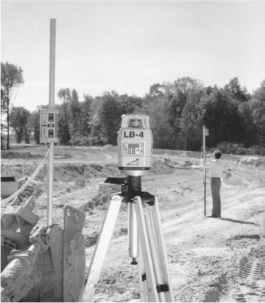
Tracking Level. The grade laser tracking level is mounted on a substantial tripod, is leveled, and delivers a rotating beam of laser light. When set for automatic operation, its beam passes over the whole area of a construction site at 6 to 40 revolutions per second (rps).
Each work crew that needs grade checks has a stadia rod, and a target with rechargeable battery that can be clamped to it, similar to that shown in Fig. 2.20.
It is of course very important that the laser beam elevation be accurate. The instrument is set up in somewhat the same manner as a self-leveling engineers’ level, by adjustment of three leveling screws. It is turned on, and allowed a 2-minute warmup period before being placed in automatic rotation.
This rotation may shut off automatically if the instrument is disturbed.
A rod and target are set on a benchmark, and a reading is taken. If the elevation is a fractional number, it can be rounded off for greater convenience by lifting or lowering the laser slightly, using a fine vertical adjustment on top of the motor head.
The laser may have a distance range adjustment, which should be correct for job conditions. It may cover an area from 600- to 2000-foot (183- to 610-meters) in diameter.
Oscillation. When work areas are typically long and narrow, as in trenching or highway jobs, the laser head may oscillate from side to side, in an arc of 30° or more, instead of rotating.
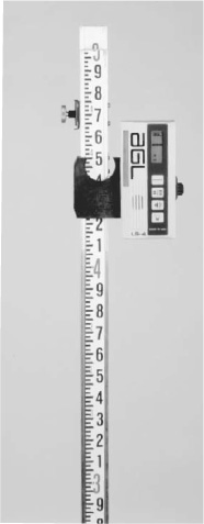
FIGURE 2.20 Target on surveyor’s rod. (Courtesy of AGL Lasers.)
FIGURE 2.21 Grade Laser Beacon and targets. (Courtesy of Laser Alignment Inc.)
This oscillation may be quite rapid, and is used more often in automatic control of depth of excavation than as a reference for work crews.
Grade Laser Beacon. The Grade Laser Beacon manufactured by Laser Alignment Inc. is useful in a variety of ways on agricultural and construction jobs. The model shown in Fig. 2.21 is being used for site grading. Seen in that figure are uses with a target on a surveyor’s rod and a receiver mounted on a grading machine. The beacon is portable and self-leveling, and indicates when elevation changes have occurred by a disturbance. It is waterproof, can be set for two separate alignment sights, and is workable for an area of 2,000-foot (610-m) diameter. In addition to site preparation work, it is useful for agricultural land leveling, construction slope control, and ditch excavation.
The laser beam rotation control can be adjusted to 6, 12, 20, or 40 revolutions per second (rps) for optimum performance. It would be set at lower rps to save battery life, but the higher speed is needed for use with fast-moving equipment using the laser beam received by hydraulic sensors to adjust for cutting grade. This use with equipment will be explained shortly. The manual adjustments by the equipment operator may be done with a slower laser rps. But the faster the beam rotation, the quicker the grading equipment response, preventing a washboard effect on the graded surface.
For slope control the Grade Laser Beacon is directed up perhaps a 2:1 or 3:1 slope to guide the grading machine or surveyor’s rod holder. The slope grade can be set at a range from –4 to + 50 percent. This instrument can be set with two grades set simultaneously on the illuminated grade display. That is useful when two pipelines coming together have different slopes, for example, the feeder lines and the main pipeline. In another case the side slopes for a ditch will probably be steeper than the bottom area running to the water trickle channel.
Automatic Grade Control. The basic application of the rotating laser beam is the direct, automatic control of cutting depth (or filling height) of grading machines.
The machine to be controlled must have hydraulic lift for its cutting edge or parts. A vertical mast is erected on a frame resting on the edge, and is kept vertical by a pendulum-controlled valve and hydraulic minicylinders. It has a telescopic adjustment for height.
The mast carries a receiver with a number of cells sensitive to the laser light, which are wired to a solenoid valve that controls the hoist for the cutting edge. This valve opens almost instantaneously when activated by the receiver cells.
Center cells are neutral or on grade indicators, and do not activate the valve. Those just above or just below center will open the valve for 50 milliseconds or  second. The top and bottom ones open it for 200 milliseconds or ⅕ second.
There may be additional cells to activate a control that will swivel the mast to keep the receiver facing the laser.
The mast height is adjusted so that the center of the receiver is in the plane of the laser beam when the cutting edge is exactly on grade, as seen in Fig. 2.22.
The machine is then driven and steered in the normal manner. If the blade drops slightly below grade, the hoist valve will be opened for second to raise it. This action will be repeated 5 times per second until it is on grade.
If the drop is enough to activate the top cells, they will open the valve for ⅕ second. If the demand for lift is repeated when the beam returns, the valve will stay open continuously until correction shifts the work to the -second adjustment, or to neutral.
If the blade moves above grade, similar action will put the valve in the down position. Lights keep the operator informed of the actions of the system.
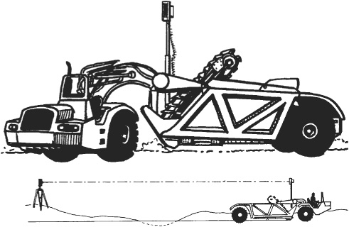
FIGURE 2.22 Laser-controlled scraper.
A refinement for fast-moving machines (scraper or dozer) is a proportional current system, responding to the 10-sweeps-per-second or faster laser. In this, the opening of the valve is proportional to the amount of correction needed.
Repetition of automatic adjustments 5 or 10 times per second results in running a very accurate grade, usually within 0.02 or 0.04 of specification. Accuracy is greatest close in, and declines within these limits to a distance of 1,000 feet (305 m), the longest recommended.
With increasing distance, the beam widens so as to lose its pinpoint accuracy, and problems with diffraction become more likely. Errors caused by curvature of the earth’s surface are given in Fig. 2.28.
Applications. This system is well adapted to automatic control of ditchers, landplanes, scrapers, dozers, tube and cable plows, and graders.
The grader requires an additional cross-slope sensor. The laser controls the lift cylinder for the leading edge, while the slope regulator keeps the trailing edge in proper relationship.
Automatic control is largely limited to finishing operations, as it is not designed to sense loads, and may therefore tend to make a machine dig into more material than it can move.
When the automatic control overloads the machine, the operator can override it, and raise the blade. The operator can then return for additional manually controlled passes, finally returning it to automatic for trimming.
Excavating Trench. To excavate a trench to a given depth and in a specified alignment, Laser Alignment Inc. provides a laser instrument called the Depthmaster, depicted in Fig. 2.23. It can be attached to the dipper stick of a hydraulic excavator and gets direction from a laser beacon, described previously, set up nearby.
The Depthmaster gives readings for vertical alignment and depth of cut. The vertical alignment is noted by the three lights at the bottom of the readout panel. If the middle light shows, the excavating dipper is in alignment, whereas the left or right light would indicate that a move to extend or retract is needed. The depth of cut is indicated by the display of light in the strip of lights up and down on the panel. When the dipper is not in the laser beacon’s beam because it is too high, or low, no depth light will be lighted. If the light with a horizontal bar on it is lighted, then the bucket in a horizontal digging position is at the correct excavating depth. If one of the upper or lower lights is lighted, then the bucket will have to be lowered or raised to be on grade.
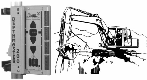
FIGURE 2.23 Depthmaster—attached to excavator. (Courtesy of Laser Alignment Inc.)
The Depthmaster gives a constant accuracy “on grade” to ± 1/6 inch or ± ½ inch (+/–4.2 mm or +/–12.7 mm) depending on the job site requirements. It has 9 inches (229 mm) of vertical receiving cells and can receive from any laser in all directions, that is, 360° horizontally. The power used for this instrument is 11 to 30 volts direct current, and its operating range is 1,000 feet (305 m) from the laser. The operator can have a readout panel in the cab of his or her hydraulic excavator in case there is difficulty reading the Depthmaster on the dipper stick.
The global positioning system (GPS) is a satellite-based system developed for military use but successfully transferred for many civilian uses. GPS makes use of 24 satellites. Commercial uses include land surveying, vehicle navigation and tracking, mining and construction, agricultural systems, and many other applications.
GPS Methods. Mobile GPS receivers can be mounted on earthmoving or agricultural equipment. The receivers obtain positions by using the signals from the GPS satellites. Two-dimensional positions (latitude and longitude) use the signals from three satellites, and three-dimensional positions (latitude, longitude, and elevation) require signals from four satellites. GPS positions are based on a technique called trilateration, which is similar to triangulation but is based on the distances to the satellites, not angles. GPS hardware has very accurate clocks, so timing of these satellite signals is known very accurately. The GPS receiver calculates the distance to satellites, using the signals from them and their location in the sky. Those distances are then used to calculate the receiver’s location on earth.
Differential GPS. A technique called differential GPS (DGPS) is used for guiding earthmoving, mining, and agricultural equipment. DGPS can be used to obtain positions with the accuracy and dynamic positioning needed for vehicle guidance. DGPS requires a base station with a precisely known location. This base station calculates its GPS position from the satellite signals, compares the calculated position with its known position, and generates correction data. The correction data are broadcast by radio in real time to the GPS receivers nearby, for example, on earthmoving equipment. All mobile GPS receivers within range of the radio broadcast can use correction from a single base station. See Fig. 2.24.
Accuracy. High-quality GPS receivers can receive two types of signals from the satellites: C/A code or carrier phase. With DGPS, the accuracy for C/A code receivers can be improved to ½ meter (1.64 ft), and can be up to 10 meters (32.8 ft) at ranges over 1000 kilometers (621 miles) from the base station. Carrier-phase receivers can have an accuracy to 5 millimeters (0.2 inches), and move out to 5 centimeters (2 inches) at ranges of 10 to 15 kilometers (6.2 to 9.3 miles) from the base station. The important development of real-time kinematic (RTK) allows users to obtain centimeter-accuracy GPS positions in the dynamic mode. With RTK, land surveyors can accurately map property boundaries by simply walking or driving around the property. The location of a piece of earthmoving equipment can be monitored on a real-time basis by the operator.
Mobile Unit Links. Several types of communication links can be used between the base station and the mobile GPS receiver. The contractor can use UHF and VHF radio modems or cellular phones to establish the link between the base station and the mobile receiver. Near coastlines and navigable waterways, governments broadcast DGPS correction data on frequencies between 283.5 and 325 kilohertz. In addition, in many areas there are commercial services which broadcast DGPS data on an FM subcarrier or by satellite.
Construction Uses. In earthmoving, the main uses of GPS for machine guidance are for grade control on dozers, scrapers, and motor graders. Traditionally, the transfer of engineering design from the drawing board or computer design to the field has relied on the accurate placement of stakes by survey teams. With the use of centimeter-accuracy guidance on board the earthmoving machine, the operator can visualize the position of cut-and-fill surfaces in relation to the earthwork design. This allows a complete digital link from design to layout and reduces the time for which expensive machines stand idle or need to move the earth material a second time. Moreover, real-time information can be obtained on the location and productivity of earthmoving equipment, allowing improved management of the construction site.
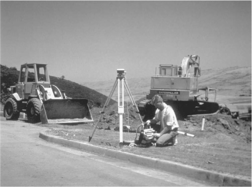
FIGURE 2.24 Setting a GPS base station. (Courtesy of Trimble Navigation Limited.)
Connected Community. The Trimble Navigation Ltd company has developed this ability for the construction community of players in conjunction with their GPS systems. It provides a means of getting new plan information to all players who need to know the information, i.e. players on the job site or in the office, inspectors, suppliers, et al.
The introduction that makes this possible is a rugged controller and office software linked to Trimble’s LM80 Layout Manager, which links, in real time, two-way data transfer between project designers in the office and the construction personnel in the field. The LM80 creates a digital replica of the project blueprint. Therefore, design engineers can make authorized changes immediately available to the construction personnel and the other players who need to know of them so they can be implemented.
Automatic control systems are now available for ditchers, i.e. trenchers, land planes, scrapers, dozers, tube and cable plows, and graders. The Leica Geosystems features trench tool modes that guide the operator where to trench or backfill and helps him or her to avoid over-digging. The AccuGrade developed by Caterpillar can have a variety of guides for motor-grader operators. The basic system provides cross grade slope control. When combined with AccuGrade elevation controls, it provides automatic elevation controls for both ends of the grader’s blade. Apache Technologies has developed their CB52 dual control box that controls the lift and tilt of a skid steer loader, compact track loader, or dozer blade.
Specific Equipment Applications. For cutting a specified slope accurately for earthwork, Topcon’s Touch Series 5 (TS5) can be used. It involves a Touch Control Panel (TCP) at the operator’s station on the excavator, a valve control box on the machine to regulate the hydraulic system of the excavator, and three machine sensors to direct the required angles of the machine parts (boom, dipper stick, and bucket, see Fig. 2.25) to achieve the desired positions as set on the TCP. The automatic controls set the excavator so it does not overcut nor undercut the slope, making for extra work to get the desired result.
The TCP can also be programmed for a fixed depth of basement, footing, or the bottom of a pipe trench. with a display screen to show the bucket position relative to the desired grade, even when the excavator is making “blind cuts,” where the operator cannot see the bottom.
Another application is for the TS5 instruments on a grader to automatically grade the subgrade for a pavement. The TS5 consists of a control box, like the TCP, four machine sensors, and an all new High Flow hydraulic valve package. The sensors are on the blade and supports in all their positions for grading. The grader operator uses the control box to enter the desired elevation and slope that TS5 will maintain.
When the machine begins grading, information from each of the four sensors is sent to the control box where comparisons are made to the desired grade entered by the operator. If necessary, the control box sends out correction signals to the hydraulic valves to adjust the blade to the required grade. The TS5 actually performs the measurements and corrections more than 30 times a second so that the grader can move at a relatively high speed.
The Leica Geosystems GPS base station receives time and place information from the GPS satellites in the sky. The base station, which is standard, modem survey equipment, communicates via radio modem to all machines. The precise position is computed on the machine relative to the base station and is then combined with slope and other sensors to determine the exact position and heading of the grader’s blade.

FIGURE 2.25 Depth and slope control. By knowing the lengths of each machine member and accurately measuring the angles between them, the control system precisely and automatically positions the bucket to any depth and slope. (Courtesy of Topcon Positioning Systems.)
By comparing these values to the project data stored in the computer on board the grader, corrections for height and cross slope are transmitted to the SonicMaster blade controller, also on board, freeing the operator to concentrate on steering. Only one or two passes are required to get to final grade. And the result provides accuracy of +/– 0.10 feet (+/– 3 cm) in height for rough grading. A more refined Grade Star TPS solution provides accuracy to +/– 0.02 feet (+/– 6.1 mm) in height and +/– 0.04 feet (+/– 12.2 mm) for position.
Distance from the roving grader is constrained by the strength of the radio link, from 1,000 feet (305 m) up to six miles (9.7 km).
Several battery-powered instruments are available that can read the distance to a target by measuring reflection time of multiple-phase signals.
The short-range Cubitape uses a modulated infrared light source, for distances up to 6,000 feet (1.83 km), with differences in range depending on the type of target and atmospheric conditions. The target is located by means of a built-in telescope.
The distance is automatically displayed in digits for feet (or meters) and their decimal fractions. See Fig. 2.26.
The Electrotape (Fig. 2.27) uses a microwave beam for distances of 100 feet (30.5 m) to 30 miles (48.3 km). Two identical instruments are used, with built-in short wave communication between them for the operators. The readings are taken first by one unit, then by the other, as an accuracy check.
These instruments measure direct line-of-sight (slope) distances. If there is a difference in elevation between the points, the horizontal distance must be calculated.
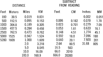
Correction for the curve of the earth’s surface is needed if elevations are required. An approximate formula, good up to distances of a few hundred miles, is
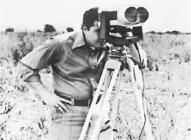
FIGURE 2.26 Cubitape. (Courtesy of Cubic Industrial Corp.)
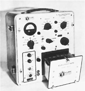
FIGURE 2.27 Electrotape. (Courtesy of Cubic Industrial Corp.)
FIGURE 2.28 Corrections for curve of earth’s surface.
Figure 2.28 is a table for various distances. The correction is subtracted from the apparent eleva -tion indicated by the instrument. It will be noted that the curvature is very slight within ordinary survey distances, but must be considered in long sights.
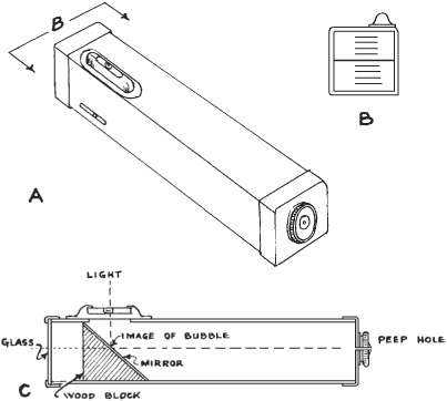
Hand Level. Rough levels may also be run with hand levels, such as the one shown in Fig. 2.29. This consists of a sighting tube, in the top of which is a small spirit level parallel with the line of sight. A slanted mirror reflects the spirit level so that it is seen vertically beside the field of view. The object glass is marked with a centerline, and may have two or more stadia lines.
This level is used by holding it to one eye, and tipping it up or down until the bubble is centered at the centerline on the glass. Any object cut by this line is then on a level with the observer’s eye, and nearby elevations may be determined and levels run in the same manner as with an instrument.
Results are much less accurate, but in rough work this may be more than compensated by the ease of use.
The eye height of the observer may be used as a unit of measurement. In taking the height of a hill, as in Fig. 2.30, the observer holds the level to her or his eye, while the rod operator moves up or down the hill in response to instructions, until the bottom of the rod, a stick, or the operator’s shoe rests on the ground at eye level. The spot is marked, the observer moves to it, standing with his or her heel on it, and the rod operator moves uphill, repeating the process. When the top is reached, the last observation should be taken on the rod, or a ruler or tape, to show the distance from the hilltop up to eye level. The height of the hill is the height of the observer, multiplied by the number of observations, less the rod reading on the last observation.
In working downhill, Fig. 2.30(B), a target fastened at the top of the rod, or a mark on a long stick, is sighted and moved until it is level with the eye. The observer then moves to that spot, while the target is moved downhill until level with the new position. On the last sight, the distance from the ground to eye level is measured.
Each observation covers a drop equal to the height of the target minus the height of the observer, and they will all be equal except the last one, which should be separately figured and added to the others.
An individual’s eye height, measured from the heel when she or he is in erect position, will seldom vary more than an inch, which is not too large an error for rough work. Care should be taken that the heel, and not the ball of the foot, is placed on the mark.
Level Clinometer. The clinometer is a special type of hand level which can be used to measure slopes and vertical angles. The spirit level is hinged so that it can be rotated about 45° in either direction, and a pointer and scale indicate the angle between the spirit level and the line of sight. The bubble will appear at the centerline of the object glass when the hand level is held at the angle indicated by the scale. The scale is usually graduated to indicate both angles and slopes.
The angle of a slope may be measured by setting a target at eye height at one end and sighting it from the other. With the centerline on the target, the spirit level may be adjusted until the bubble is beside the line. The pointer on the scale will then indicate the slope of the hill.
It may also be used as an inclinometer by placing it on the slope to be measured, and setting the spirit level until the bubble is centered. It is usually good practice to lay a board on the ground surface and take its slope to eliminate the effect of small irregularities.
String Level. A string level is convenient to use over short distances. It is a spirit level fitted with prongs by which it can be hung from a string stretched tightly between two marks. Elevations may be taken from the end of the string, or by measuring down from any part of it, as illustrated in Fig. 2.31.
The string used should be strong enough to take sufficient pull to remove all sag. If it is at all slack, it will give false readings, showing slope at the ends of a level stretch and level somewhere near the middle of an inclined string. A special need is depicted in Fig. 2.32.
FIGURE 2.30 Using a hand level.
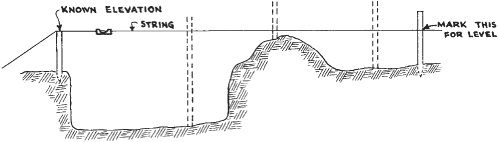
FIGURE 2.31 Using a string level.
FIGURE 2.32 Figuring string heights on banked curve. (Courtesy of CMI Corp.)
Most string levels use flexible prongs which are easily bent by light pressure. It is therefore best to check such a level before every use, and occasionally during a job. This is done by leveling a string according to it, slacking the string and reversing the direction of the level on it, and tightening the string to the same marks. If the reading is the same, the level is all right. If it disagrees, bend a prong sufficiently to move the bubble one-quarter of the way to the center, then move the string to center the bubble. Reverse the level on the string, and repeat the procedure as above, until the reading is the same both ways.
Carpenters’ Level. A carpenters’ level may be used to level a string, although not as conveniently. A string leveled by a carpenters’ level may be used for direct adjustment of a string level.
Altimeter. Altimeters or barometers which are small enough to be carried, and sensitive enough to react to small changes in elevation, may be used for taking preliminary levels.
The most convenient altimeters are mountaineers’ pocket models, the size of a large watch. Engineers’ models, which are rather rare, have a glass for magnifying the scale, for fine reading.
An altimeter is set for correct or assumed altitude when work with it is started. As it is carried up- or downhill, the hands will point to higher or lower altitudes on the scale, and notes may be made of the reading whenever desired. It is advisable to tap the instrument before each reading.
Altimeters provide the quickest and easiest means of finding heights and depths in rugged and overgrown country. They are not accurate enough to be used in setting grades, except in very experienced hands.
A stringline is a string or wire that indicates location, grade, or both location and grade. Its use in construction is widespread and very old. A familiar example is string stretched between batter boards for reference in laying foundations and pipes.
A stringline may serve as a visual guide for a machine operator to prevent him or her from running off-line between widely spaced stakes. If the machine is equipped with a pointer or a suspended plumb bob on the frame of its grading blade, ditching wheel, or other grade-making tool, it can be adjusted so that following the string accurately with it ensures working to proper alignment and grade.
The principal and increasing use of stringlines has been in automatic control of grading, excavating, and paving machines. These controls, which are described in Chapter. 19, are usually made up of a tracer or wand that stays in contact with the string, and a sensor that reacts to any change in tracer position by actuating hydraulic valves to restore proper relationship with the string.
A machine may need two stringlines, one at each side. However, if it has an automatic cross-slope control, only one line is required.
Accuracy in locating such stringlines is of the utmost importance, as line and grade produced in the automatic operation are absolutely dependent on it.
There are various ways of setting up a stringline. The following description follows a booklet, Stringline Manual, published by CMI Corporation.
Apparatus. The string holder is made up of a metal stake [standard length 42 inches (107 cm)], a sliding bracket that can be secured to the stake with a setscrew, and a horizontal rod that slides in the bracket, and can be locked in it with another screw. One end of the rod is notched to hold the string.
The string is usually a special yellow polyethylene selected for strength, stretch characteristics, visibility, and rot resistance. Regular strong white cord may be substituted in an emergency.
The string is carried between jobs on storage reels. When in position, it is tightened by means of take-up reels, one at each end. See Fig. 2.33.
An engineers’ steel rule is used to measure the distance from string down to the top of the grade stake (tack line). This distance has been previously determined, and it is the same for each grade stake in a section.
A plumb bob may or may not be used for horizontal alignment.
Location. The stringline is placed outside the strip or lane being graded. In highway work, this usually means in the shoulder, 2 or more feet (0.61 or more meters) beyond the edge of the lane. It is preferably 18 to 30 inches (46 to 76 cm) above grade, although some machines can use higher and lower settings. It should be at least 5 inches (12.7 cm) above the ground.
It may be possible to use one setting for up to three processes—subgrade finishing, laying selected subbase, and paving. Clearance from lane edge must be sufficient to accommodate windrowing and removing of waste material, passage of machine tracks if outside the lane, and minimum tracing arm lengths.
Stakes are driven about 1 foot outside of the line proposed for string, alongside marking hubs or grade stakes.
Hubs (Grade Stakes). Hubs are usually 2×2 (51×51 mm) wood stakes, placed by surveyors along the line of the string, parallel to the roadway centerline. They are driven to grade (bluetops) or to some fixed distance, the same for each stake, above grade. They are usually spaced 50 feet (15.2 m) apart for uncomplicated work, and 25 feet (7.62 m) for superelevations, vertical curves, and other special situations.
Reference grade is level with the centerline on straightaways. On superelevated (banked) curves, the reference is to the tipped plane of the cross section, so that it will be lower than the near edge on the inside of a curve, and higher than it on the outside (Fig. 2.32).
A tack is driven into the top of each hub for precise location of horizontal alignment.
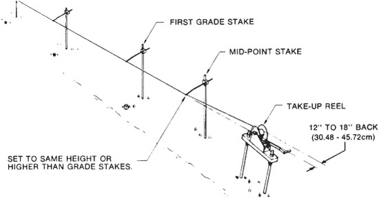
FIGURE 2.33 Stringline and take-up reel. (Courtesy of CMI Corp.)
Setting Up. A string stake is driven alongside each hub, about 1 foot (0.305 m) to the outside. It must be vertical, and driven deep enough for good stability. The rod should extend directly toward the stake, and can be slid inward or outward until its slotted end is directly over the tack. The bracket is raised or lowered until the rod is ¼ (6.4 mm) inch above the selected stringline height. Adjustments are locked with setscrews.
A steel engineers’ rule is used to measure the height of the rod, and to check its location over the tack.
Take-up reels are then placed, 25 feet (7.62 m) before the first stake in the section, and 25 feet (7.62 m) past the last stake. These should be offset 12 to 18 inches (30 to 46 cm) beyond the end of the line of the string, with the crank to the outside. The reel is first located on the ground, stakes are driven through holes in its base, and it is then raised to a convenient cranking height, and clamped.
A metal midpoint stake is driven in line with the string stakes, halfway between the last (or the first) one and the reel. The rod may be at stringline grade, or higher.
The string itself is reeled off a storage reel (or two reels if there are two lines) held on a bar on a truck. It is anchored by winding about 25 feet (7.62 m) onto one of the take-up reels, and is paid out as the truck drives to a few feet beyond the other end. The string is cut and secured to that reel.
The string is pulled taut by hand and by turning the reels. Then it is inserted into each rod notch. It should slip into them easily, but require moderate force to be pulled out. Slot openings can be widened with a screwdriver, or narrowed with pliers. There should be no visible sag between stakes.
Using an engineers’ rule, adjust the rod brackets so that the string is at its exact height above the tacks, and with a plumb bob to make sure it is in line. Sight down the completed line, and recheck any break in a smooth flow.
Visual inspection should be repeated just before use, and occasionally as work progresses.
Any breaks in the string can be repaired by relaxing the tension, tying the broken ends together with a square knot, and retightening.
Distance. Surface distances may be measured approximately by pacing, stadia, or car speedometer; or more exactly by tape (chaining), the distance meters mentioned earlier, or measuring wheel.
Distances may also be read off job plans or maps. But a possibility of an error in a map, or in interpreting it or its scale, must be guarded against.
A measuring wheel is a convenient and sufficiently accurate means for measuring both short and long distances. Small wheels are hand-rolled along the ground, while large ones may be either hand-rolled or towed slowly by a vehicle. A counter registers the distance covered in feet (5.1 cm). Readings down to 2 inches (5.1 cm) may be obtained. See Fig. 2.34.
Bank. A bank of earth or other material may be measured before and during the time it is dug away. This is usually done to establish a basis for payment to the owner of the land, or from the job to which it is being hauled.
A grid is established before digging starts. Ten- or even 5-foot (3.05-m or even 1.52-m) intervals are used between stakes for close measurement of rough ground, and wider spacing for more even ground and less exact work.
Benchmarks and reference points are established well outside of the digging area. Then the elevation of the ground is taken at each stake. Elevations are also taken of humps or hollows lying between the stakes. A contour map is usually made, and ground elevations are plotted on cross-section paper. Vertical scale may be exaggerated. This original surface, called grade, is a solid line, as in Fig. 2.35. Any desired profile or section that does not follow the stake lines can be made up from the contour map. The new elevations are plotted on the same paper as the originals, and are usually indicated by dotted lines, as illustrated.
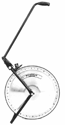
FIGURE 2.34 Measuring wheel. (Courtesy of Rolatape, Inc.)
Excavated material has been removed from between the solid and the dotted lines on each of the profiles. This area is measured by counting squares, dividing into rectangles and triangles, or mechanical methods. If the horizontal scale is 1 inch (25.4 mm) to 25 feet (7.6 m), and the vertical scale 1 inch (25.4 mm) to 5 feet (1.52 m), a square inch indicates 125 square feet (11.6 sq.m). It is best to keep the figuring in feet until the end, for greater accuracy.
The vertical area is determined for each profile, then areas are added and the total is divided by their number to obtain an average. This average is multiplied by the length of the excavation at right angles to the profiles. This gives the amount excavated in cubic feet. Dividing it by 27 reduces it to cubic yards, bank measure.
The same procedure is followed each time the bank is measured. On all calculations after the first it is usual to determine both the amount removed since the previous measurement, and the total amount removed since the job began.
Pile. An experienced estimator can often judge the volume of a pile quite accurately by inspection, without measurement. However, appearances are often deceptive, and most people are safer if they make at least approximate measurements as a check.
Piles can often be conveniently measured by calculating the volume of regular masses of similar outline, and making plus or minus adjustments for differences.
A pile of clean, dry sand may have a conical shape, or be a ridge with a triangular cross section, ending in half cones. Measurements should be taken to determine base size and height. See Fig. 2.36.
The area of the circular base of a cone is found approximately from the circumference by the formula
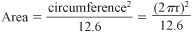
and from one-half the diameter by
Area = 3.14 × radius2
The volume of a cone is the height times one-third the base area.
The long part of the pile is figured by the formula

A long pile will have the volume of the center section, plus the volume of one cone, as each of the ends is a half cone.
When the pile shape is flattened, different, or irregular, profiles and cross sections are taken in the same manner described for banks.
In the construction industry the word “production” is assigned the same meaning as “output,” which is defined in the dictionary as “the quantity or amount produced, as in a given time.” Perhaps a better definition for these words in construction is “useful work accomplished,” as in the early stages of a job the chief product is likely to be destruction and upheaval.
Production may be figured in at least three ways. First is on the basis of job requirements. If a time schedule allows 200 working days to move 3,000,000 yards (2,300,000 cu.m) of earth, the contractor’s earthmoving machines must move or “produce” 15,000 yards (11,500 cu.m) per day. Second, the production of a certain machine is measured or estimated, to determine the number of such machines needed to meet the production required. If a certain scraper can move 1,000 yards (765 cu.m) a day under this job’s conditions, the contractor must keep at least 15 of them working at that rate.
The third way of figuring production is in terms of cost. This is the final and important calculation, as it is the basis on which contracts are let, and on which contractors ride in Cadillacs or go broke. But cost calculations are unlikely to be accurate or useful until job conditions and equipment are known.
Earthmoving quantities may be measured in terms of bulk of material, weight of material, area to be worked, or lineal feet or yards processed.
Cubic Measure. Most earthmoving is computed in cubic yards. A cubic yard is a cube 3 feet (0.91 m) long, 3 feet (0.91 m) wide, and 3 feet (0.91 m) high. It is about 6 inches (15.2 cm) greater in each dimension than the space occupied by a card table.
“Cubic yard” may be stated and written in full, but is usually shortened to “yard” or abbreviated to cu. yd. or cy. The full designation is used in discussions where the type of yard might be in doubt, as where there is a possibility of confusion with square yards or linear yards. Abbreviations are used in formulas, figuring, and texts where terms are frequently repeated.
Cubic yards may refer to bank, loose, or compacted measure. This will be discussed under Swell and Shrinkage.
Many dimensions in field measurements and contract plans are in feet, so that if they are multiplied together to obtain bulk, results are obtained in cubic feet.
These are usually changed to cubic yards by dividing by 27 [there are 27 cubic feet (0.76 cu.m) in 1 cubic yard]. Of course it is also possible to divide the original linear measurements by 3 to convert them into yards, and then multiply, but this may lead to working in fractions, decimals, and mixed numbers.
Most countries use metric measures. See pages A.4 and A.18. One meter is 39.37 inches, 3.2808 feet, or 1.0936 yards. A cubic meter is 35.315 cubic feet or 1.308 cubic yards, a bit less than ⅓ yards.
Measurements are sometimes given in feet and inches. A cubic inch is too small a unit to be used for dirt (it takes 1,728 of them to make a cubic foot, 46,656 of them to make a cubic yard), but it is used in measurements of engine and compressor displacement and other mechanical descriptions.
It is difficult to multiply feet and inches by feet and inches, so the inches are expressed as either regular or decimal fractions of feet. Regular fractions (⅔,  , etc.) are more accurate, decimals are more convenient.
Weight. In highway jobs, cellar excavation, and site preparation the estimator is chiefly interested in the bulk and digging characteristics of the material to be moved. Its weight has importance chiefly in figuring loading and gradability of haulers, and is only occasionally used as the basis for estimating. See Fig. 3.5.
In mines and quarries weight is likely to be a more important factor than bulk. Products such as coal, crushed stone, cement, ores, and ore concentrates are usually sold by weight, and therefore are measured by weight as they are dug. There are exceptions, however. Some open-pit mines compute their operations on a yardage basis. Others figure ore by the ton and overburden by the yard.
The standard weight measurement is the short ton of 2,000 pounds (907 kg). There is also a long ton of 2,240 pounds (1,017 kg) that is used in some mines. It should always be specified as a long ton, and the unmodified word “ton” should mean short ton only.
Other measures are the hundredweight of 100 pounds (45.4 kg), and the British stone that weighs 14 pounds (6.36 kg). In the metric system a kilogram, often called a kilo, is 2.2046 pounds, say 2.2 for short. A metric ton is 1,000 kilograms, or 2,204.6 pounds, about 10 percent more weight than in a short ton, and a little less than a long ton.
Area. In many operations, bulk and weight do not provide a suitable basis for measuring the amount of work. For example, with any given land-clearing condition, the time and cost of the work vary with the area. Clearing is usually measured by the acre, which is 43,560 square feet (4,047 sq.m). Many estimators do their figuring in acres of 40,000 square feet to simplify arithmetic, and make allowance afterward for the difference of almost 10 percent.
Grading land where cuts and fills are shallow is likely to show costs in relation to area rather than bulk of soil to be moved. But when cuts and fills are deep, bulk becomes more important than area. Exact grade requirements increase grading costs in proportion to area. The estimator must keep track of these factors.
Topsoiling and seeding are figured mostly on the basis of area, although of course the depth of topsoil and the heaviness of seeding are important in determining the rate per square yard.
In the metric system the square yard is replaced by the square meter. This contains 10.76 square feet or 1.196 (say 1.2) square yards. The next larger measure is the “are” that contains 100 square meters, 119.6 square yards, or .0247 acre. Then there is the hectare, that contains 10,000 square meters, 11,960 square yards, or 2.451 (say 2½) acres. The largest measurement is the square kilometer, 1,000,000 square meters, 245.1 acres, or .3861 (say ⅖) square mile.
Lineal Measurement. Work such as ditching, installing pipe, tile, and fencing is measured by the lineal or running foot, yard, or mile. There are 3 feet in a yard, and 5,280 feet or 1,760 yards in a mile. Metric measures are the meter, 39.37 inches, 3.28 feet, or 1.09 yards; and the kilometer, that is 1,000 meters, 3,281 feet, 1,094 yards, or .6212 (slightly more than ⅗) mile.
From both a time and cost viewpoint it is of course necessary to know also the width and depth of the ditch, the soil and other special conditions, the size and type of pipe, and the type and quality of fencing.
Drilling is usually measured by the lineal foot (or meter), with the size of hole specified.
A construction machine may work in an intermittent cycle, in a continuous flow, or in ways that are intermediate between the two types. Figure 2.37 shows the category in which various types of equipment fall.
Intermittent Cycle. This group includes the most important machines used in primary excavation. They each have a bucket, bowl, or body that is loaded, moved, dumped, and returned to the loading point. One complete set of operations is called a work cycle.
For example, a revolving shovel digs in the bank, swings the bucket over a truck body, dumps it, swings back to the bank, and positions the bucket to dig. A scraper loads in the cut, travels to the fill, dumps, turns, returns to the cut, turns, and gets in position to load. In each case, the set of operations is a cycle.
Production rate depends on the size and efficiency of the earthmoving container, whether bucket, bowl, blade or belt, and the time it takes to go through a complete cycle. The cycle time in turn, depends on the rate at which the container is loaded, moved, dumped, and returned to the loading point.
The distance the load must be moved may be a few feet (meters) in the swing of the shovel, or a number of miles (kilometers) in truck haulage. Distance is often the determining factor in the production cycle.
The size of the container is rated by the manufacturer, usually for level and for heaped loads. Container efficiency is the amount of actual load in relation to rated load, and will be discussed later.
The probable production of a machine can be calculated by multiplying its actual capacity by the number of times it can go through its cycle in a given period. Actual production may be found by measurement in the bank, the haulers, or the fill of material removed during a measured time, and/or by measurement of individual loads and timing of cycles.
Continuous Flow. Continuous flow is found chiefly in equipment using belts, pumps, and/or pipes. It includes machines such as wheel ditchers that dig by means of individual buckets, but which have a number of buckets digging at the same time. The individual bucket cycles overlap, and production is continuous.
Production of a belt machine is found by averaging a number of measurements of the cross section of the load on the belt, and multiplying this figure by the speed of the belt in feet per minute.
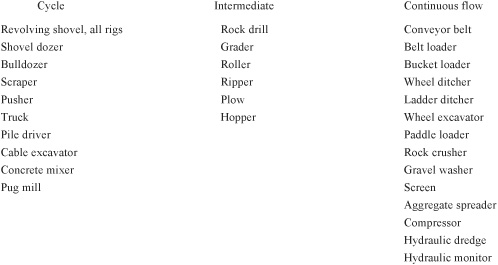
FIGURE 2.37 Cycle classification.
The cross section is usually measured in square feet (sq.m), so the result is divided by 27 to obtain loose cubic yards (cu.m).
Ditchers, bucket conveyors, and other machines using numerous small buckets may be checked by multiplying bucket capacity by the number of buckets per minute, or by measuring the load going through a discharge belt or chute.
Measurements may also be made in the bank, in haulers, or in the fill.
In dredging, the volume of water handled is computed by multiplying a cross section of the stream in the pipe by the rate of flow. This production in cubic feet or cubic yards of water per minute is then multiplied by the percentage of solids in the water—usually 10 to 20 percent—to obtain useful production.
Each belt or pipe might be considered to be a container with a measurable capacity. However, this capacity is related to haul distance rather than rate of production. A conveyor belt carrying a load with a cross section of 2 square feet (0.19 sq.m) and traveling 500 feet per minute (152 m/min.) will deliver 1,000 cubic feet per minute (28.3 cu.m/min.), regardless of whether it is a 10-foot (3 m) feeder belt or a half-mile-long (0.80 km long) hauler. The only production difference is the extra time—practically 5 minutes—that it will take to reload the longer belt after unloading it at the end of a shift.
The cost of belt construction and maintenance varies almost directly with the length if width, load, and support requirements remain the same.
Intermediate. This class of machines requires individual methods of study to determine production.
A grader is a continuous flow machine in sidecasting until it reaches the end of a work area and must turn or reverse. If the area is very short, or it is pushing material bulldozer fashion, it has a cycle. Most grader work is measured by the area processed, either as square yards or as linear feet of roadway of a specified width. Production may be figured on a basis of width processed times speed.
A drill will cut continuously to the end of its stroke, but steels are changed and/or new holes are started frequently. Measurement is by speed in feet per minute or per hour, less nondrilling time.
A hopper often serves to convert intermittent cycle loads to continuous flow, as in a dragline feeding a conveyor belt. Its production rate is usually that of either the excavator or the belt, as it can be adjusted to almost any rate of feed within its capacity.
A special application is in speeding up truck loading. A 2-yard (1.53 cu.m) excavator might load sand into a hopper at the rate of 3 yards (2.3 cu.m) a minute, and the hopper might be able to fill a 15-yard (11.5 cu.m) truck in 1 minute. It serves to convert a rapidly repeated 2-yard (1.53 cu.m) shovel cycle into a slower 15-yard (11.5 cu.m) truck cycle.
Noncycle Time. There is almost always a wide gap between production that should be obtained on a basis of cycle speed and capacity, and what is actually produced. Checking the cause of these delays is a drawn-out matter that can usually be best done by studying lost-time reports made out by operators or checkers. Some, however, are frequent enough to be included in brief time studies.
For a shovel there are cleanup and move-up operations, and waits for trucks. Trucks wait to get into loading position, are delayed by traffic, and get stuck. Scrapers wait for pushers, have traffic problems, and sometimes get stuck.
If a breakdown occurs, it is useful to make a note of its nature, and of how long how many machines are put out of action or slowed down.
Swell. When soil or rock is dug or blasted out of its original position, it breaks up into particles or chunks that lie loosely on each other. This rearrangement creates spaces or voids and adds to its bulk. This increase from bank yards to loose yards is called “swell.”
Swell is expressed as a percentage of the bulk in the bank. If 1 bank yard puffs up to ¼ loose yards, the swell is ¼ × 100 percent, or 25 percent.
When converting bank yards to loose yards, the measurement is increased by the percentage of swell. In the above example, 10 bank yards (7.65 bank cu.m) could be converted to 10 + 10 × .25, or 10 × 1.25, giving 12.5 loose yards (9.56 loose cu.m).
Swell Factor. The swell factor is the percentage of bank yards in loose yards. The contractor uses it to make a conversion on paper of the loose yards being hauled back to the bank yards for which he or she may be getting paid. The swell factor is found by dividing the bulk of a bank yard by the bulk of a loose yard, per the formula

If the swell is 25 percent,

The percentage of voids is found by subtracting the swell factor from 1.00.
The tables provided in Fig. 2.38 show average swell, swell factor, and voids for various classes of soil. It also shows the shrinkage factor, which is the reduction in bulk to compacted yards in a fill.
Shrinkage. When soil placed in a fill is thoroughly compacted by rolling, it will shrink, the amount of shrinkage depending on its character, its structure in the bank, the thickness of fill layers, and the weight and type of roller. Blasted rock may retain some swell, while ordinary loam may be reduced to 80 or 90 percent of bank volume. Measurement in the fill is described as compacted yards, or yards after shrinkage.
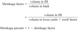
Shrinkage may also occur in undisturbed soil on which fills are placed, particularly if 50 tons (45,400 kg) plus superrollers are used. Such shrinkage may be calculated by the following formula, if more exact information is lacking:

This is just an averaging of maximum compaction at the top and zero compaction just below where the effect is felt. This depth would be about 48 inches (1.2 m) in a clay loam soil under a 50-ton (45,400 kg) roller. Such soil may have a shrinkage factor of .2, so by this formula

FIGURE 2.38 Soil swell and shrinkage.
In wet conditions, or on steep slopes, displacement of subgrade material to the side may reduce its useful bulk much more than its compaction does.
Exceptional Soils. Soils composed of volcanic ash or pumice, and soils built up by streams on flats in arid regions, may show very peculiar behavior. Particularly, they may show excessive compaction, sometimes to 40 percent of bank volume. In some cases, they even show shrinkage during digging, so that loose yards are heavier than bank yards (cubic meters).
Such soils are found only in limited areas where contractors may be aware of their possibilities. However, they constitute a hazard for the estimator, and any indication of their existence on a job should be carefully checked.
One western state highway department in the United States has adopted a policy of paying for highway borrow by weight rather than by volume to avoid unpleasant surprises for either the budget or the contractor when such materials appear in borrow pits. The necessity of measurement before starting work is avoided also. Portable truck scales that can be set up in a few minutes are used for measurement of pay quantities.
“Container” is used here as a broad term to include transporting boxes such as truck bodies, digging and carrying buckets or bowls as in shovels and scrapers, and digging and pushing blades on dozers and graders. But it does not include belts or pipes.
Measurement. Most buckets and bodies are rated by the manufacturer as to carrying capacity in loose yards. This rating may be water level (the yardage of liquid which could be carried if it did not leak out), line of plate or struck measure, which is water level plus any space between parts of the rim which project above its low point, or heaped.
Shovel dipper buckets and highway truck bodies are normally rated at water level, carrying scrapers and off-the-road trucks at both struck and heaped measure, and clamshells at water level, line of plate and heaped.
Body capacity should be indicated by a printed plate. It is usually in yards, but may be in cubic feet. It ordinarily does not include sideboards, or other removable extensions which increase its volume. The extra load between added boards may be found by the proportion between the heights of the body wall and of the board. For example, if a straight-sided body with 4-foot (1.2 m) sides holds 8 yards (6.1 cu.m), a 1-foot (30.5-cm) sideboard added on each side will increase capacity by one-fourth, or 2 yards (1.5 cu.m).
If there is no plate, size can be determined by measurement of the inside length, width, and height, usually in feet and fractions of feet. These are multiplied together, to obtain cubic feet that are divided by 27 to get cubic yards.
Heaps. The heap on top of a load can be measured only approximately because of its shape. It is usually calculated on the basis of an assumed even slope of the material. The slopes from opposite sides are continued until they meet. In general, the volume of a heap is determined by the slope of the material and the area of the body. A steep slope and a wide body give it maximum yardage.
According to S.A.E. (Society of Automotive Engineers) standards, a heap is figured on a basis of slopes of 3 to 1 (3 horizontal feet to each foot of rise) inward from the top of the body walls. This covers most conditions, but some materials will stack up much higher, particularly if the trip is short and smooth, as in a dragline bucket, which a few will slide or flow to flatter slopes as the container is moved or shaken.
Truck Bodies. Bodies such as are mounted on highway trucks have a rectangular floor and vertical body walls, with provision for increasing the height of sidewalls by adding wood or metal extensions. The rear wall (tailgate) is hinged to dump the load when the body is raised at the front. Most of such bodies are 7 feet (2.1 m) wide inside. Some standard heights and capacities are shown in Fig. 2.39.
Bodies of off-the-road trucks are difficult to measure, as they may slope outward from bottom to top and the sloped fixed tailboard ends at a much lower level than the body sides. Ratings generally assume a load struck off by a plank resting on the two sides and moved from front to rear. In the absence of indications to the contrary, manufacturers’ ratings for struck load may be accepted.
The more important rating for off-the-road trucks is capacity in tons. This is usually 1½ times the rating in yards. The trucks are designed to carry a certain payload, and the body is designed to carry that load in material that weighs 3,000 pounds (1.360 kg) to the loose yard. Lighter materials can be heaped, heavier materials should not fill the body completely. Bodies can be purchased in special sizes for regular handling of material of very different weights.
Capacity Tests. When a capacity test is to be run, the bank is trimmed and measured and a number of approximately equal loads are taken and counted. The bank is then trimmed off and measured again, and the difference calculated in yards. Then
FIGURE 2.39 Capacity of standard truck bodies.
Such tests should be run on the largest practical volume for best accuracy. Minimum amount would be about 200 yards (153 cu.m). Counting of excavator bucket loads during the test will supply container and output data for it also.
Scraper Bowl. Scraper bowls are irregular in shape and in height of rim. Manufacturers’ rating on struck load may be accepted if known. If not, inside measurements are taken and capacity is worked out, making allowance for curves and irregularities.
Scrapers are usually rated for heaps with 1-to-1 slopes, 3 times as steep as the S.A.E. standard. Dirt may stand a little more steeply above a scraper because of the way it is crowded up from the bottom, but there is no justification for assuming that it can stand on such a slope, either at the moment of loading or during the shaking and vibration of a haul. Also, such slopes are never carried up to peaks.
A good rule of thumb is to take the scraper’s maximum heap at one-half the manufacturer’s rating. That is, a scraper rated at 20 yards (15.3 cu.m) struck and 28 yards (21.4 cu.m) heaped can be assumed to have a heaped capacity of up to 24 loose yards (18.4 cu.m), unless there are definite indications to the contrary. If swell factor were .80, the heaped load would contain 19.2 bank yards (14.7 cu.m). Extensive checking by the U.S. Bureau of Public Roads indicates that scraper loads in bank yards seldom equal their rated struck capacity, so this works out well enough.
Push loading compacts material, so for the same heap a scraper carries fewer bank yards if it is loaded from the top.
Shovel Bucket. Shovel buckets are rated at struck measure, in yards and fractions of yards. Size can be checked fairly accurately by measuring and multiplying length, width, and height, as in the case of the truck body. Taper, curves, and extension of the lip can be used to increase the result to the nearest ¼ yard (0.19 cu.m). Heaps, when digging conditions permit, range between one-eighth and one-fourth of struck capacity.
Hoe buckets are rated and measured in the same manner. Heaps are usually small or absent. Width is an important factor in loading efficiency. Deep narrow buckets may average loads less than one-third of rated capacity.
The open front of the dragline bucket makes it difficult to measure accurately, as the capacity is determined largely by the steepness of slope of the load. A chunky mud that can bulge over the teeth and pile steeply over the top may have almost as much in the heap as there is in the struck load.
Clamshell buckets may be rated water level with the end plates, struck measure along the tops of the sides, or heaped. Another rating that may be important is that of deck area—the length and breadth of the space on a level floor occupied by the bucket when fully open. The same space is required between braces in a trench.
Loader Bucket. Front-end loader buckets are rated at struck capacity across the sidewalls. If the bucket can be tipped back 20 degrees or more at ground level, and digging conditions and tractor stability permit, it can carry a very large heap, perhaps 50 percent of struck capacity. A bucket that will not tip back seldom can take one-eighth more than struck capacity. However, in hard digging few buckets can pick up even a struck load, and tractor stability may not permit carrying an overload. On the average these buckets are underloaded by loose measurement more often than they are heaped.
Dozer Blade. The capacity of a bulldozer blade cannot be computed exactly. The blade forms only one of the six sides of a shapeless payload. Since the load must slide or roll along the ground, friction is a very important limiting factor on load size. Materials with low internal friction or light weight, and downhill pushing favor big loads. Pushing through a slot or between windrows, or with the blade almost touching that of another dozer, increases load by reducing side spillage.
A good average load may be said to be 20 percent more than would be measured by the full width and height of the blade, with a forward slope of 1-to-1. The actual load would be higher in the center and skimped in at the corners, averaging out as above. See Fig. 2.40.
The blade on a 25-ton (22,700 kg) bulldozer might be 12 feet (3.7 m) wide and 4½ feet (1.4 m) high. The profile of the theoretical load would be a right triangle 4½ by 4½, with an area of 10.25 square feet (0.95 sq.m). Multiplying this by the 12-foot (3.7 m) blade width, we have 123 cubic feet (3.5 cu.m). Adding 20 percent for center bulges, this would be 148 cubic feet (4.2 cu.m) or 5.5 loose cubic yards. Different manufacturers rate blades of this size at 5 to 7½ loose yards (3.8 to 5.7 cu.m).
Under very good conditions the load might average 6 inches (15.2 cm) higher than the blade top, and extend forward on a 1½-to-1 slope. Then the profile would be 5 feet × 7½ feet or 37.5 square feet (3.5 sq.m). Multiplying by 12-foot (3.7 m) width, we get 230 cubic feet (6.5 cu.m) or about 8½ yards loose.
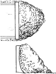
FIGURE 2.40 Bulldozer blade load.
Capacity of a blade is greatly affected by grade. Downhill the load tends to slide along with minimum pressure; uphill its friction rises and it spills more off the sides. Possible load, both from standpoint of power to push it and ability to keep it in front of the blade, increases about 4 percent for each percent of down slope. That is, a dozer might push double its normal load down a 25 percent grade.
Uphill the load falls off at first almost as rapidly, but the decline slows with steeper grades. A half load might be pushed up a 20 percent grade, and a quarter load up 100 percent.
When a job is in progress, dozer blade capacity can be checked by counting the number of full passes required to dig a known yardage of a bank, or by counting loads pushed into a pile and measuring the pile.
The first result will be in bank yards, the second in loose yards (cubic meters).
Container Efficiency. A machine may go through many production cycles with less than its rated load. The ratio of the container’s capacity to its actual load in loose yards is called the efficiency factor of the bucket, bowl, or body.
An excavator may not be able to load its bucket or bowl fully because of hard digging, inadequate power, improper design, dull teeth, traction, heavy material, operator’s haste or carelessness, or combinations of these and other unfavorable conditions.
A truck may be run partly empty to enable it to climb steep grades, to reduce strain on rough ground, to cross soft ground, to increase haul speed, or because of poor mechanical or tire conditions.
When material is coarse in proportion to bucket size, chunks may be partly supported by the sides and each other, leaving excessive voids and reducing the actual load below that indicated by the capacity of the container and the bulk of the load. The container efficiency factor (CEF) formula is
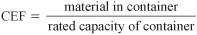
The amount of material in the container may be determined by careful measurement and/or weighing of a number of individual loads, or by measuring either the bank or the fill to determine the amount of material moved in a certain number of cycles.
For example, a ½-yard (0.4-cu.m) backhoe might dig a ditch section 2½ feet (0.8 m) wide, 6 feet (1.8 m) deep and 12 feet (3.4 m) long in 25 cycles, removing 180 cubic feet (5.1 cu.m) or 6.67 cubic yards bank measure. Dividing 6.67 by 25, we have an average bucket load of .267 yard (0.2 cu.m). Since the rated capacity of the bucket is .5 yard (0.4 cu.m), we have

The efficiency factor in loose yards would be greater by the percentage of swell. In clay loam with 20 percent swell (see below) the loose yards would be 6.67 × 1.20, or 8.0 (6.1 cu.m). Dividing by 25 cycles, we would have an average load of .32 loose yard (0.24 cu.m). Then

It is important to always specify whether any container efficiency factor is for loose yards or bank yards. One may be readily converted to the other, the loose yards figure almost always being the larger, as it is increased by the percentage of swell.
Work Cycles. The work cycle may be timed as a whole in figuring output for existing conditions. For accuracy it is necessary to take the average of a large number of passes as there may be a considerable variation among them.
If a study is made of a cycle, either to find a way to speed it up, or to use its time intervals as a basis for figuring production under different conditions, it can be broken down into individual operations which are timed separately.
A study of bulldozer and of scraper operation may include some or all of the divisions listed below. Each one should be timed. Digging and traveling distances should be measured. A record should be made of all grades, as these machines are much less efficient going uphill than downhill.
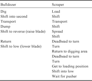
Machine Efficiency. Nonworking time such as delays for moving the machine, minor repair ad justment, rest, getting instructions, or looking at grade stakes is not averaged into cycle time. It is considered separately as the efficiency factor of the machine. It may work out between 70 and 85 percent for short periods with expert operators on a properly run job, with machinery in good condition and weather favorable.
A convenient way of making rule-of-thumb allowance for efficiency of about 83 percent is to consider that 1 hour contains only 50 working minutes. On this basis, a machine with a 30-second cycle cannot be expected to perform it more than 100 times per hour.
If two machines are interdependent, the efficiency factor is usually lower so far as the job is concerned. If two 80 percent efficient machines are down at the same time every time, the efficiency factor remains at 80 percent. If they are down separately each time, the factor drops to 60 percent.
As the period under study becomes longer, efficiency drops steadily, as weather, work sequence stoppages, and major overhauls must be considered. Time losses can be further increased by in -efficient management, bad pit layout, poor morale of employees, or other unfavorable conditions.
Output Formulas. A formula which can be used for figuring production of any machine with a regular cycle is
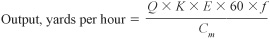
where Q = capacity, either struck or heaped
K = efficiency factor of bucket or body
E = efficiency factor of machine
60 = minutes in 1 hour
f = soil conversion factor
Cm = cycle time, minutes
If the result is to be in bank yards (cubic meters), f has a value obtained from observed swell, or from Fig. 2.38. If the result is to be in loose yards, f equals 1, and can be dropped from the equation. The factor K is not required when full, solid loads can be taken. If efficiency is approximated at ⅘, then 50 minutes are used instead of 60, for the hour.
Under these conditions, the following simplified formula can be used:
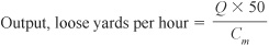
If a 45-minute hour is used, this formula is

When timing machines have a cycle less than a minute, it is more convenient to figure it in seconds. This is done by multiplying the number of minutes by 60, and using Cs—cycle time in seconds—instead of Cm. With these substitutions, the formula will be
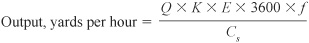
Or simplified for a 50-minute hour to

For a 45-minute hour we would have
Additional data on output will be found in Chapter. 11 and the Appendix, and included in discussions of particular machines.