
Amo, amas, amat; amamus, amatis, amant. Three persons, each both singular and plural, make Six. For Latin lovers, Six is sex, and in soixante-neuf, even the numeral is erotic. Those Indo-European roots suggest that Six, like sex, is connected with cutting and dividing. Six is the first number with more than one factor, capable of division in different ways. It is the number of choice, change and chance.
Life depends on the nucleus with six protons, surrounded by an outer electronic shell which is just half-empty, half-full. The twos and fours of quantum mechanics allow the carbon atom to bond to oxygen. But carbon dating works energetically with other atoms, with just the right chemistry for the complex molecules of life. Equally penetrating and penetrated, carbon atoms bind happily to other carbon atoms, with what in the Sixties was called polymorphous perversity.
Diamonds may be your best friend, but there are alternative forms of bonding. In 1985 a new form of pure carbon, called C60 for its 60 atoms, was identified. It’s odd that it took chemists so long to spot this molecule, because, like quasi-crystals, it had already been anticipated in theory, and because the polyhedral geometry was so familiar after the 1970 World Cup. Many had been getting their kicks with Six:
Every carbon atom in a molecule of C60 lies on one pentagon and two hexagons. It turned out that this secret passage from Five-ness to Six-ness had been sitting in burnt toast all the time, unrecognised.
Six is two threes, and six is three twos. The multiplication of numbers is insensitive to order: first doubling and then tripling is the same as first tripling and then doubling. If we add further structure, two threes are not the same as three twos. In music, Holst evokes mercuriality in ‘Mercury’ by suddenly shifting from 2 × 3 to 3 × 2 rhythm (and also hopping unexpectedly by six semitones from Bb to E). This is rather contrived, but more natural three-against-two effects are common in Latin American dance. As a crossover compromise, West Side Story has the cross-rhythm of ‘I want to live in America’.
There is an analogue in a sort of twisted multiplication which first occurs when Six comes into the picture. There is a problem in geometry that could crop up when assembling furniture from a flatpack. Suppose you have a flat triangular piece which has to slot into the rest of the design, but you cannot see which way round or even which way up it goes. There are six possibilities to try out. On top of the general difficulty of following flatpack instructions, an inescapable mathematical fact can make this totally confusing. Rotating the triangle, then flipping it over, does one thing. But giving it the flip first, and then the rotation, ends up with something else. Operations, unlike numbers, are sensitive to order. As soon as Galois, Abel and Hamilton started writing symbols for operations, a serious new algebra began with twisted multiplication: a × b may not be the same as b × a.
We have already touched on this twisting with the quaternions in Chapter 4. They have just this ‘non-commuting’ property, because they represent rotations in three dimensions. The flatpack operations can be thought of as picking just six quaternions which form a closed group. The question of how many such sets of operations exist, starts off a huge area of modern algebra which must be indicated with just a few images. One picture is of the crystals and their symmetries in three dimensions. Crystals are classified by rotation and reflection symmetries, and the reason why quasi-crystals were such a surprise, is that being aperiodic they failed to fit into this classification. But crystals are only the start: there are rotations in spaces of any number of dimensions, and the analogues of crystals. The non-commuting of rotations in the quark’s colour space is an essential feature underlying the confinement of the nuclear force. This in turn points the way to the geometry of string theory, where physicists hope to find symmetries related to the fundamental particles and forces.
There is a wonderful image of the complexity of such questions in the Rubik cube, with its non-commuting twisting operations. It was the Sudoku of the 1980s. For the standard 3 × 3 × 3 Rubik cube there are, it turns out, 43252003274489856000 possible positions. Solving the puzzle amounts to finding a path from one position to another amongst this number, the order of twisting operations being crucial. Like Sudoku, it also gave a thought-provoking image of how fascinating logical puzzles can be, in a way that official education completely misses. Schools banned it, and young people developing an amazing intuition for its geometry were laughed at.
Meanwhile, in the 1980s, algebraists were finally sorting out what turned out to be a kind of Rubik cube at the centre of mathematical reality. There are certain structures, enormous extensions of the flatpack problem, which are to rotations rather as the primes are to numbers: these are the finite simple groups. They are very special, definite, extremely large and complicated structures, still full of mysteries and new discoveries. They culminate in the Monster group which has 246 × 320 × 59 × 76 X 112 X 133 × 17 × 19 × 23 × 29 × 31 × 41 × 47 × 59 × 71 = 80801742479451 2875886459904961710757005754368000000000 elements, rather than the six of the flatpack.
Sudoku is a very much simpler problem, but it still presents huge numbers of ways in which the numbers 1 to 9 can be combined, to be sorted out systematically. The number Six is a good starting point for seeing how changes and choices combine. They naturally lead on to the questions about chances. Less obviously, they will also lead back to the duality of growth and oscillation, and from there to primes, powers, dimensions and spheres, and then back to life.
In Killer Sudoku you may find a box of three cells where the numbers must add to 6. The numbers then must be 1 + 2 + 3 = 6 (thus showing 6 as a triangular number). But the 1, 2 and 3 may be in any of the six orders: 123, 132, 213, 231, 312, 321.
There are six orders because 6 = 1 × 2 × 3, and this fact is what makes 6 the starting point for permutations and combinations. Before embarking on this, it’s worth remarking on the coincidence that
6 = 1 + 2 + 3 = 1 × 2 × 3.
This property is tantamount to the fact that six is what the Greeks called a perfect number. Constance Reid chose this feature for Chapter 6 of From Zero to Infinity, leading into an unexpected tale about the ‘Mersenne primes’. We will return to this in Chapter 8. In this chapter, we explore the complexity rather than the perfection of Six.
We say that 6 is ‘3 factorial’ and write 3! as shorthand for 1 × 2 × 3. Why is this the number of orderings of three things? It is easy to write them out and count them, but it is better to argue systematically. The first can be 1, 2 or 3; once this is chosen there are two possibilities for the second, and then there is only one choice for the third. This is like a tree with three branches, each dividing into two, and each of these ending in one leaf: this gives a total of 3 × 2 × 1 leaves. The same argument works for the number of ways of ordering four things:
4! = 4 × 3 × 2 × 1 = 24.
Instead of working these out from scratch, we can recycle the work already done: 4! is 4 × 3!, and then 5! is 5 × 4!, and so on:
5! = 5 × 4 × 3 × 2 × 1 = 5 × 4! = 120
6! = 6 × 5 × 4 × 3 × 2 × 1 = 6 × 5! = 720
7! = 5040, 8! = 40320, 9! = 362880.
This last number gives the total number of possible rows (or columns, or subsquares) of Sudoku.
You can get a picture of these numbers from the task of ringing the changes on a set of bells. Enthusiasts take about three hours to toil through the 5040 permutations on seven bells; to do justice to eight bells would take a day. If you are an interrogator for the ‘American-led coalition’, given to playing continuous music to your captives to induce them to confess, you might consider an interesting variant. In the atonal twelve-tone music popularised by Schönberg, a composition is based on the twelve notes of the chromatic scale arranged in some order. There are 12! = 479001600 such ‘tone rows’ and it would take around 30 years to play them. After this, a new generation of interrogators could take over in the long task of fighting the war on terror.
Alternatively, Sudoku could provide a suitable life-long task. By developing these counting procedures, it has been found that there are 6670903752021072936960 patterns for 3 × 3 Sudoku: in solving a puzzle you are rejecting all but one of these possibilities. However, you might say some of these patterns are essentially the same. They differ only through the permutations of columns or rows, a rotation of the square, or a renaming of the symbols. The accepted figure for the number of essentially different patterns is 5472730538.
EASY: For n ≥ 5, n! always ends with a 0.
DIFFICULT: There are many zeroes at the end of 100! and 1000!
- how many? (Hint: do not work these numbers out.)
A cube has complete symmetry between its six faces. This symmetry determines the properties of dice, with six equally likely outcomes, each having a probability of 1/6. In passing, it is worth noting that there are four other shapes with such complete symmetry: tetrahedron, octahedron, dodecahedron and icosahedron. But they lack the practical convenience of cubes. So that six-faced cube makes a natural link between the counting of possibilities, and the measuring of chances through the theory of probability.
The meaning of ‘probability’ and ‘randomness’ is not as simple as one might like. Sometimes probability is used as if equivalent to frequency or prevalence. That’s absolutely true, as far as anyone knows, when randomness derives from a quantum-mechanical measurement. In the case of dice, however, randomness means only that the outcome depends in such a complicated way on how they are shaken and thrown that in practice it cannot be predicted. This, ultimately, depends upon the chaotic nature of physical systems, and the sensitive dependence of outcomes on initial conditions. So it has its limitations.
If dice-throwing was studied as intensively as golf swings, perhaps there would be champions in achieving double-sixes. (Conversely, if I played golf the results would be about as good as throwing dice.) An example on the borderline of randomness arises in the playing of roulette. This is intended by casino operators to be a game of pure luck, but in the 1980s a group of scientists noticed that because bets can be placed after the ball has been set rolling, it is actually possible to make a quick prediction and take advantage of it. They smuggled in a computer, and until thrown out of Las Vegas, made good money out of science.
A deeper problem is that sometimes the word ‘probability’ is used for describing a state of belief, rather than something observed and measured. This question of whether probability is objective or subjective goes back to its earliest days. It is natural to use this more subjective meaning in situations where there will only be one outcome, as yet unknown—for instance, the future climate of the planet. Controversy about the forecasts of the Intergovernmental Panel on Climate Change has so far not focused on its definitions of probabilities, but it is worth noting that this is a difficult question, taken very seriously by climate scientists. They have developed methods for calculating probabilities for outcomes, based on taking large ensembles of slightly different models, parallel Earths with slightly different assumptions. The IPCC also includes a more subjective element in its quantification of expert confidence in the conclusions reached. It is hard to see quite how these numbers can be tested by any actual measurement, or based on frequency.
It is a relief to turn from an area where probability is vitally important, but difficult to rationalise completely, to one which is generally foolish, but crystal clear. Probability has a perfect illustration in the casino, and for many people their most intense encounter with numbers comes in—well, the numbers game. And as it happens, the past decade has seen an explosion in the gambling business, with the British government promoting it as an economic lifeline for regions such as Manchester which were once proud centres of science and industry. (A parallel development of gaming and gambling has changed the agricultural and manufacturing America known to Constance Reid in the 1950s.)
In the British national lottery, the prizes depend on guessing which six numbered balls will be spewed out randomly (as far as one can judge) with much razzmatazz from an urn of 49. Neglecting all questions of bonus numbers and secondary prizes, we can ask how many possibilities there are for these six balls, and so the probability of guessing them correctly.
There are 49 possibilities for the first ball to emerge from the urn, then 48 for the second, 47 for the third; 46, 45, and 44 for the remaining three. This makes 49 × 48 × 47 × 46 × 45 × 44 possibilities. But this is overcounting: the order in which they emerge is irrelevant. There are 6! possible orders, so the complete number of possible sets of six balls is

This is written more neatly as

and this expression tells a story: it shows a symmetry between the 43 and the 6. This is a basic yes-or-no symmetry inherent in the problem. When you fill in the lottery card, you may do it either by choosing the six to be marked, or the 43 not to be marked, and the result will be the same.
This number can be worked out as 13983816. Assuming these outcomes are equally likely—as they are unless the lottery is as corrupt as football—a punter buying one card and marking it with six guesses has a chance of one in 13983816 of winning the lottery prize.
If you play over and over again, the average value of the entry card will be the value of the prize, divided by 13983816. This is less than the price of the card, but of course people don’t buy lottery tickets for their average value, but for the pleasure of knowing that there is a non-zero probability of their lives being transformed by wealth. (They can also derive satisfaction from contributing to the arts, sports and community projects funded from the lottery profits.)
The lottery promoter caters further to irrationality by publicising the numbers that have come up more often in the past. I do not know whether punters consider it a good idea to choose such numbers because they are lucky, or whether they believe such numbers should be avoided because ‘by the law of averages’ they are less likely to appear in the future. Both lines of thought are misguided: assuming that the balls are juggled properly, the past record has no influence on the future. If Mars or Mithras have a soft spot for you, and can nudge electrons to make the balls in the urn emerge in line with your ticket, then you are on to a good thing. Otherwise, there are no lucky or unlucky numbers. Your best bet is to pick numbers that you think other, more foolish people will avoid. Then in the unlikely event of winning, your prize will not be shared.
As the lottery shows, combinatorial numbers based on just a few elements can easily reach astronomical proportions. Another example comes in solving anagrams for crossword puzzles. A fifteen-letter anagram can need up to 15! = 1307674368000 possibilities to be considered. In Umberto Eco’s novel Foucault’s Pendulum there is a discussion of a ‘giant computer’ for such tasks. But you don’t need a computer, still less a giant one, for crosswords. This is because you can break these numbers down as quickly as they are built up, using features of language to eliminate huge numbers of possibilities at once.
This is why code-breaking is possible. Simple cryptograms, based on substituting one letter for another, can be made in 26! different ways, which means that to break one you have to locate the correct solution out of 403291461126605635584000000 possibilities. This figure suggests an impossible task, but you can solve such puzzles with a message of 30 or so letters, by such observations as that E is the most common letter, QKZ is an unlikely pattern, and so on. In contrast, the four-digit PIN security used on mobile phones cannot be broken down, so that celebrity-stalking journalists are forced to go through 10000 possibilities to get at their targets unless they can make a lucky guess.
These ideas, and the number six in particular, have played a vital part in world history. The Enigma enciphering machine, as adapted for German military use during the mid-1930s, had three rotors which could be used in any order, giving six possibilities. Polish mathematicians developed a brilliant method for breaking the resulting ciphered messages, but this depended on there being only these six rotor-order choices. When in 1938 the Germans added two alternative rotors, the choices went up from 3 × 2 × 1 to 5 × 4 × 3, a tenfold increase. The Poles had to pass the problem on to the British, who soon developed code-breaking into a great strategic asset, but were likewise stretched by a further increase to 8 × 7 × 6. These numbers were critical: the code-breaking process was on a knife-edge of practicability. If there had been 10 × 9 × 8 rotor choices from the start, the Poles would never have been able to get going.
The general point lying behind these figures is that if combinatorial numbers have to be matched by the scale of physical resources (in the number of people, pieces of equipment, or time taken) then the task may well be impossible. The German designers of the military Enigma believed they had devised a scheme that would ensure just such security. The complexity of the machine was enhanced by an extra plugboard which performed a further scrambling operation. A typical plugboard setting consisted of a choice of ten pairs of letters. Since every such choice created a different code, the code-breaker had to work out what choice had been made. The number of ways of choosing ten pairs out of 26 letters is

which is indeed astronomical.
DEADLY: Why is this? If 13 pairs were used rather than 10, would the number of possibilities be increased?
Sometimes people refer to these enormous figures as ‘the odds against breaking the Enigma’. This is highly misleading. One would not measure the odds against completing a crossword puzzle by looking at the probability of finding the solution by filling in letters at random. The structure of a crossword puzzle can be broken down, and so, it turned out, could the logic of the plugboard.
Alan Turing, who has already made more than one appearance, was the British mathematician who achieved this feat. He and another mathematician, Gordon Welchman, found a logical method of dealing with all plugboard choices at once. It was remarkably similar to the work of solving Sudoku by following a chain of logical deductions based on consistency requirements. Turing’s method depended on knowing for certain the plaintext for around 25 letters of an Enigma message, very like the 25 or so numbers generally given as initial information for a Sudoku puzzle. You might wonder whether this means that Enigma-solving could be used as a newspaper puzzle. There are two reasons why not: one is that the technicality of the Enigma wirings, needed for the logical deductions, makes this infeasible as a pencil-and-paper problem. Another is that Turing’s method for attacking an Enigma message required solving not just one Sudoku-like puzzle, but perhaps millions. (The scale of this number is given by 8 × 7 × 6 × 263, the number of possible rotor settings.) Still, the difficulty of Sudoku gives a good picture of the logical complexity of Turing’s method. The fact that it could be implemented on a machine with 1940s technology, breaking a message in hours rather than weeks, was vital to the SecondWorld War.
All animals and plants have evolved to cope with uncertainty. Using probability theory to enhance human capacities doesn’t mean behaving recklessly: it means using reason and patience. Turing’s probability theory gave vital extra tools for adding up faint clues to Enigma-enciphered messages: it was the appliance of science. But culture has a problem with probability, and displays highly ambivalent and contradictory attitudes. Entrepreneurs reward themselves as risk-takers, yet the markets are said to hate uncertainty. ‘Security’ is the word round which governments spin.
Ambivalence about gambling is particularly conspicuous. Being based on pure chance, involving no skill whatsoever, and pandering to irrational arguments, the lottery has emphasised the dubious value of reason and education. It is, for some reason, greatly encouraged. But other games require enormous skill, and are, equally unaccountably, considered disreputable. Poker, which has boomed through Internet gaming, is one such.
Although the hands dealt in any one game are a matter of chance, a serious player will in the long run succeed by rational application of the laws of probability. Online play eliminates the human element of poker-face nods and winks, although it introduces the problem of not being able to see whether other players are colluding. It is a model of what business is supposed to be like, rewarding patience, investment, rational strategic decisions and a cool nerve in the face of occasional loss. Cool students rightly find this more a rewarding form of income than stacking supermarket shelves or providing escort services.
Notwithstanding these observations, an English court adjudicated in January 2007 that as the cards are shuffled, poker is a game of luck and not of skill. This is a judgment which is tantamount to rejecting the 500 years of mathematical probability theory, not to mention the insurance and financial industries which depend on it. (One of the most striking developments of mathematics since the 1980s, now providing lucrative employment for many graduates, is in the ‘stochastic theory’ of mathematical finance. It is based entirely on concepts of random behaviour.) Meanwhile the American legislature effectively criminalised on-line poker, sending its London-based finances into a nosedive.
The law can be an ass, but the laws of probability are rational, and poker gives good examples of how they can be applied. A typical problem, found on a poker website, is: ‘What is the probability that a five-card poker hand contains at least one ace?’ To solve it, consider the chance of a no-ace hand. The calculation can be summarised like this: there is a probability of 48/52 that the first card is not an ace, then 47/51 that the second is not an ace, and so on for the remaining three cards. The probability of five not-ace cards is the product (48 × 47 × 46 × 45 × 44)/(52 × 51 × 50 × 49 × 48) = 0.658842 … so the chance of at least one ace is 0.341158…
The analysis of problems like this is much assisted by the idea of conditional probabilities. Given that you have one ace, what is the probability that an opponent has two? Such calculations can be used to measure the value of information. Indeed, Turing’s deepest contribution to the code-breaking work lay in showing how to define this measure by objective, numerical procedures, and so turn it from an art into a mathematical science.
Valuable mathematics can be found even in the much simpler game of Snap. Two packs of 52 cards are shuffled and each dealt out one at a time simultaneously: a snap is when the two cards coincide. This is a game for children (such as I played with my granny while Constance Reid was writing her book in the 1950s) but let’s be grown-up and pretend we are betting on the number of snaps that occur during the stretch of 52 cards. If this was a television programme I could dramatise this tame game as Strip Snap, or as some globetrotting tale about defusing bombs or Russian roulette. More seriously, you might see it as related to real problems like matching segments of DNA.
In fact, suppose we are placing bets on there being no snap at all in the 52-card run. What odds should you accept? Is a snap virtually certain, or most unlikely?
This question is easier to investigate for packs not of 52 but of fewer cards. If there are only two cards, then there are only two possibilities: we can take the first pack to be in the order AB, and the second one is either AB or BA. So the probability of no-snap is 1/2. If there are only three cards, then we can take the first pack to be in order ABC, and there are six possible orderings for the second pack. Of these, only BCA and CAB have no snap. So in this case the probability of no-snap is 1/3. For four cards, the no-snap orderings are the nine BADC, BCDA, BDAC, CADB, CDBA, CDAB, DABC, DCAB, DCBA out of the 24. The probability of no-snap is 9/24 = 3/8 = 37.5%.
For five cards, there are 44 no-snap possibilities out of 120 (36.67%), and for six cards there are 265 out of 720 (36.81%). If you try to write these down you will realise that you need a more systematic way of counting them. This is not so easy and I’ll give the answers for seven, eight and nine cards in a way that shows the pattern:
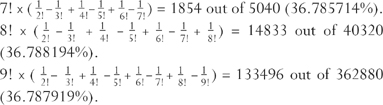
The pattern shows that it hardly makes any difference to the answer whether there are 52 cards or only five. The proportion of non-snap orderings gets closer and closer to the number given by
which to twelve decimal places is.367879441171…
There is thus a probability of about 37% of no-snap, 63% of at least one snap. The 37% figure is not an amazing number, being a middle-of-the-road figure like the proportion of people believing in the imminence of Armageddon, the dinosaurs in Noah’s Ark, and abductions by aliens. But this is one of the most fundamental numbers in mathematics. This limiting proportion of no-snap orderings (called ‘derangements’) has a special name. Actually the name is given to its reciprocal, the odds against no-snap in an infinite run. This is called e. So that probability of about 37% is called e−1, while e itself is the number 2.718281828459…
There is another fact about coincidences which is generally found astonishing: in a group of 23 people, it is more likely than not that two of them share the same birthday. But if you know about e, this should not come as such a surprise. Here is a rough (not a precise) argument: in a group of 28 people there are 378 pairs of people whom you can introduce and ask if they share a birthday. In each case there is a chance of 1/365 that they do, so your knowledge of e leads you to expect a better than 63% chance of hearing the words ‘Oh that’s incredible!’ In a group of 23 the chance is lower, but it is not surprising that it is just over 50%.
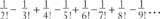
We can re-express e−1 in a more elegant way which brings out a pattern involving all the integers:

This makes sense if we define 1! = 1 and 0! = 1, so that the two extra terms just cancel each other. Remember that we have used the pattern 4! = 4 × 3!, 3! = 3 × 2!, so we can fix 1! and 0! by consistency with 2! = 2 × 1! and 1! = 1 × 0!.
The beauty of this is that by changing all the minus signs to plus signs we get another true formula:

The number e is unique in having this simple relationship between powers and permutations. The duality between + and – in these formulas should suggest a connection with the symmetries of Chapter 2. The two formulas can be rolled into one by the fuller statement that
This formula comes in naturally when we extend the scope of investigation away from simple Snap.
To do this, we return to the question of the lottery. Remember that the chance of any player winning is 1 in 13983816. Suppose first that there are exactly 13983816 players taking part. You would be right to think that the average number of winners is then 1. But in any draw, there might be 1, 2, 3 … winners—or none at all. If there are no winners, the lottery prize money is ‘rolled over’ to the next draw. What is the chance of this happening? For any individual player the probability of not winning is 13983815/13983816. Assuming that the 13983816 players make their guesses independently, the probability that they all fail to guess correctly is (13 9 8 3 8 1 5/13983816)13983816. So this is the probability of a rollover.
It turns out that this number is (almost exactly) e−1 again. Rather than try to work it out, consider the sequence of numbers (1/2)2, (2/3)3, (3/4)4, (4/5)5, (5/6)6, (6/7)7 … Your calculator will give
.25,.296296,.316406,.327680,.334898,.339917,.343609,.346439,.348678…
You can see these numbers converging, though much more slowly than the no-snap probabilities, to e-1. The more general formula comes in like this: if r × 13983816 players are participating, then the probability of a rollover is (almost exactly) e-r.
A closely related problem is this: spammers and phishers rely on there being a sucker born every minute. Suppose this is true: not that they are born regularly every 60 seconds, but randomly with an average rate of one a minute. What is the probability of a minute elapsing without a sucker being born? It is e−1. What is the probability of r minutes elapsing without a birth? It is e-r.
Another classic example of e lies in the vicious circle associated with compound interest. If tempted to consolidate your credit with the Lone Shark Finance Co., as advertised on daytime television, you should watch out. Suppose the rate is 100% per annum, with the small print saying that there shall be no lower limit on the time period on which compound interest is computed. How much interest can Mr Shark demand on £1000 after a year?
At first sight you might think it was £1000. But Mr Shark’s small print has got teeth. He could argue that the interest should be added daily, and that each day the debt increases by (1 + 1/365). At the end of the year the debt would then be £1000 × (1 + 1/365)365. At this point you might fear that by demanding hourly, minutely, secondly, nanosecondly interest the debt could be made as high as Mr Shark wanted. But e comes to your rescue—the limit as the calculation gets finer and finer is just £1000 × e. If Mr Shark’s interest rate is not 100% but r × 100%, then the limit is £1000 × er.
The last example, of vicious compound interest, shows how the number e is related to growth. This means it is also intimately connected, by the duality of growth and oscillation we met in Chapter 2, to the concept of cycles and circular motion. The full understanding of this relationship requires the full story of the complex numbers, but it is possible to pick out some illustrations without giving this complete picture. In particular, e is related to the more famous number π.
Using the complex numbers, a single, famous equation defines the relationship:

Here i means exactly the same as the complex-number pair (0, 1), described in Chapter 2 as the square root of −1. Alternatively, without using complex numbers, this equation is exactly equivalent to asserting the two properties of π:
Rather than try to go further with complex numbers, I’ll point out the way that these expressions, involving powers of π and factorials, are related to the ideas about many-dimensional spaces which have appeared in the earlier chapters.
You may be familiar with the formula that says that π is the area enclosed by a circle with unit radius. But the geometrical meaning of π is not confined to circles. It turns out that π2/2! is the hypervolume enclosed by a unit-radius 3-sphere in four dimensions, as defined in Chapter 4. The same pattern continues, so that the hypervolume enclosed by a unit (n −1)-sphere in n dimensions is:

This formula looks as if it makes no sense for odd values of n. But for n = 3, it gives the correct answer for the volume of a unit sphere (4π/3), if (3/2)! is defined to be 3/4 ×  .
.
This turns out to be a completely consistent definition: in fact (−1/2)! =  , so that (1/2)! = 1/2 × (−1/2)! = 1/2 × , and so indeed (3/2)! = 3/2 × (1/2)! = 3/4 × . The rest follow on the same pattern, giving a correct value for all the hypervolumes.
What we have done here is to extend the meaning of the! symbol for factorials, so that it is no longer defined by the number of ways of permuting a number of objects. This is very similar to the way that the concept of a power was extended in Chapter 4 from positive integers to zero, negative integers and fractions. It gives a beautiful example of how mathematics grows in surprising directions, as more subtle inter-relationships are discovered. A definition of z! can likewise be given for almost all values of z, in such a way that the relationship z! = z × (z − 1)! always holds good. This is true for complex-number values as well. One must say ‘almost all values’ because z cannot be a negative integer.
Thus the number opens the way to the measurement of hypervolumes enclosed by hyperspheres. That might seem at first sight to be of no use whatsoever, but many-dimensional spaces can be thought of as game-strategy spaces, stock-control spaces, fashion-following spaces, and generally anything from the complexity of life. A hyper-sphere is defined by extending Pythagoras’s metric into many dimensions, so the hypervolumes are all to do with sums of squares. If you are assessing how well customer demand has fitted your stock-ordering policy, then this adding up of squares is a good way to do it.
Measuring the hypervolume of a hypersphere can be thought of as measuring the probability of a random point lying inside it. So hypervolumes are naturally connected with the probability of complex events happening: statisticians use such n-dimensional spaces (called ‘degrees of freedom’) all the time. The exact mathematical result is this: suppose you have random numbers evenly spread over the range from −1 to 1. Take n such numbers, and add up their squares. The probability that this sum is less than 1 is

DIFFICULT: Work out the values for n = 2, 3, 4, 5 … Why do they decrease as n increases? How are the probabilities related to this picture?

There is an even more natural setting in which comes into life’s choices and chances. Imagine taking a random walk along a street: for each step you toss a coin to decide whether to go forward or backward. This you can take as a metaphor for the up-and-down nature of life, or as something that enters into almost any situation where many random changes are combined, for instance in the behaviour of gases, the rounding errors in a spreadsheet, or the spread of an epidemic. If you take n such random steps, it is just possible, but very unlikely, that you will go n steps in one direction. It is much more likely that you will end up near where you started. How likely? How near?
There is a useful way of visualising the possible outcomes: the Pascal Triangle. This is easily written down because every number is the sum of the two above it.
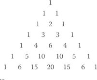
The nth row now gives the distribution of probabilities for the various possible outcomes of your n steps. Another way to visualise this triangle is as a pinball machine, with balls falling from the top and knocked randomly to left or right as they cascade downwards. They are more likely to end up in the middle than at the edge, and the numbers in the triangle give an accurate account of the distribution.
EASY: The rows add up to the powers of 2. Why is this? Find diagonals on which the entries sum to the Fibonacci numbers.
The triangle also has a direct connection with the lottery calculation we did earlier. This is because the (r + 1)th number in the nth row gives exactly the number of ways of selecting r things out of n. For instance, 13983816 would appear as the seventh number in the 49th row. I do not recommend checking this but the 6 in the fourth row gives the number of ways of choosing two out of four, and you can check there are six: (12) (13) (14) (23) (24) and (34).
As you look at larger and larger values of n, the shape made by the numbers, like the stack of balls at the bottom of a huge pinball machine, settles down to a very specific shape—often called ‘the bell curve’. Gauss discovered the universal character of this curve, which makes it the foundation of all serious statistical analysis. The formula for it involves e and π, and here is one fact which illustrates it: after an even number of steps, there is a definite probability of your random walk being back exactly where it started. (This is equivalent to the height of the central point of the pinball machine stack.) What is that probability? After n steps, it is very close to

The point is that π should not be thought of just as the measurement of a circle. It is a deep structure embedded in the numbers, bound up with growth, probability, permutations, complex numbers, and many-dimensional geometry. These subtle relationships lead to means by which it can be calculated.
The number π has always got a good press, and gets a boost from people who take great pleasure in finding and even memorising huge numbers of decimal digits, starting with 3.141592653589793238462643383279502884197 … But a question that is not so often asked is that of how these decimal digits are actually found. Although it is vaguely known that mathematicians can ‘calculate it’, how would you even begin to do the calculation? Certainly it is not obtained by measuring circles! Measurements can only have limited accuracy. Besides, general relativity tells us that space-time is everywhere curved, so the concept of a perfect circle is inconsistent with the actual physical world. The expression for e in terms of factorials gives a picture of the kind of infinite formula that must be found. But π doesn’t have such a convenient expression, and mathematicians from Archimedes onwards have been led into deeper water in trying to find practical formulas.
The startingpoint is that π is a logarithm. In fact, π is the imaginary part of the logarithm of (−1) to base e, as follows from the complex-number relation eiπ = −1.
The logarithm is the inverse of an exponential, and there are ways of inverting the formula for er, as given earlier, to obtain formulas for logarithms. These in turn lead to formulas for π. They give striking pictures of how π is interwoven with the integers, even though they are not very practical for calculations.
First comes a classic formula for squaring the circle:
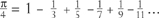
But it has a more advanced version:
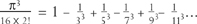
There is a similar series for every odd power. But new strange factors come in:
The numbers 1, 1, 5, 61, 1385, 50521, 2702765, 199360981, 19391512145, 2404879675441 … are the Euler numbers. They make a beautiful illustration of the interconnectedness of π with permutations, which calls for another excursion into the world of music to explain. Most well-known tunes can be identified simply by whether successive notes of the melody rise or fall. Now, in ringing the changes on six bells, sometimes the tune goes down-up-down-up-down, as for instance in the sequences:
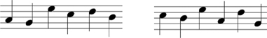
If you count the number of tunes with this property you will find just that Euler number 61. For eight bells there are 1385, for ten bells 50521, and so on.
There is a another relationship between the Euler numbers and π.
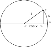
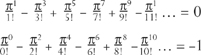
Take a circle of unit radius. Mark off a part of the circle of curved length x. It defines a straight length called cos x, as shown. As x increases from 0, cosx decreases from 1. The exact way that this happens is given by the formula:
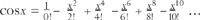
which you may notice is closely related to the formula for ex, a further aspect of the duality of growth and oscillation. If we turn this upside down, the Euler numbers appear:

You may have noticed that after the initial 1, the Euler numbers end alternately in 1 and 5. This pattern continues for ever and the final two figures also repeat in a cycle of length 10. Seeing why this is true is a more than SUPER FIENDISH puzzle. It is left as a further tantalising picture of how the patterns of primes, powers and permutations are tangled up with the number π.
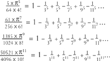
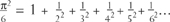
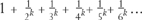
A closely related formula found by Euler, bringing us back to the number six, is
This formula is the starting point for another, quite unexpected, connection. It is related to the prime numbers. Seeing this connection needs one of the slickest pieces of algebra in all mathematics, again something found by Euler. It is as perfect as 1 + 2 + 3 = 1 × 2 × 3, turning addition into multiplication. In fact, this is just what we will do.
The first step transforms the infinite sum into an infinite multiplication:

The truth of this statement depends on the Fundamental Theorem of Arithmetic we met in Chapter 1. To see how it works, take a particular term in the infinite sum, say 1/842. It can be written as
and this product corresponds to just one of the terms that results from multiplying out all the factors in the infinite multiplication. The same applies to every integer.
The second step is to simplify these factors using a formula for infinite additions, borrowed from Chapter 9:
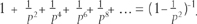
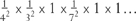
The result is best appreciated when turned upside down:
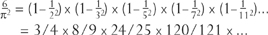
Each of the factors can be interpreted as a probability. Imagine that we pick two integers at random. The first factor, 3/4, is the probability that two numbers are not both even. The second factor, 8/9, is the probability that they are not both divisible by 3. The third factor is the probability that they are not both divisible by 5, and so on. The product of all the factors is the probability that two randomly chosen integers have no prime in common. Equivalently, it is the probability that the highest common factor of two integers is 1. This probability is.6079…, a curiously mediocre answer for such an extraordinary question.
You may wonder how probability can come into statements about primes and factors: numbers don’t have any uncertainty in their factors. The answer is that the randomness goes into the method for picking the numbers, not into the properties of the numbers you pick. It is worth spelling out what this means. First, take the numbers 1 to 9, and assume you have a method for picking one of them randomly and with equal probabilities. Choose a pair of numbers by using this method twice over. Of the 81 possible pairs, just 55 of them have a highest common factor of 1—which gives a 68% probability. The statement is that if you do the same thing for the numbers 1 to n, the proportion gets closer and closer to 6/π2 as n gets larger and larger.
There is similar argument for the probability that k integers have no prime factor in common, namely the reciprocal of
When k is even, this can be summed to a term involving πk and one of the Bernoulli numbers. These are closely connected with the Euler numbers, to the geometry of circles, and to the counting of up-and-down tunes (with an odd number of notes). The next step is to ask what happens if k is something other than an even number.
The question is closely connected with the distribution of prime numbers, which gradually become rarer and rarer. Gauss had already seen that the density of prime numbers near n behaves like the logarithm (to base e) of n. This means that for 100-figure numbers, about 1 in 230 is prime; for 200-figure numbers about 1 in 460 is prime, and so on. Other mathematicians had begun to explain this pattern, but it was Riemann who made a great advance in 1859. His method was analogous to the extension of the factorial to non-integer values. Riemann took the probability that k integers have no prime factor in common. He extended k not just to odd integers, or half-integers, but to all complex numbers. This defined the Riemann zeta-function. Using the duality of growth and oscillation, Riemann could then express the thinning out of the primes in terms of a series of waves. The mathematician Marcus du Sautoy has called these waves ‘the music of the primes’. Riemann saw that if the music takes a very particular form, much could be learnt about the infinite sequence of primes, and the exact way they thin out. This conjecture about the waves is the Riemann hypothesis.
The truth of the Riemann hypothesis is still a conjecture, and the subject of another Millennium Prize. In fact it has been a prominent problem for 100 years, and is much the oldest to attract the million-dollar bounty now. It seems to mark a frontier of the landscape that is carved out by starting with e and π, and which embodies the connections between growth, rotation, natural numbers and primes.
In a sense it is surprising that it remains unsettled because such completely new insights into numbers have emerged since Riemann’s time. Amongst all the contributors, one utterly magic figure is that of Srinavasa Ramanujan. He wrote to Hardy out of the blue from Madras in 1912—13 with a gallery of completely new formulas, presented as faits accomplis, since he rarely gave proofs. For Hardy it was rather like Turner getting a preview of the Turner Prize. Ramanujan had an extraordinary intuition not just for numbers, but for relationships which emerge on going beyond the landscape of the exponential function, and into the mountain range formed by the elliptic functions. This is territory which, 100 later, is central to mathematical discovery.
As a glimpse of new relationships, he could see why  is almost an integer, being 3964 − 104.000000177 … On the basis of this, Ramanujan found a formula for π, which gives a far quicker way of calculating it:

Ramanujan noted this in about 1913, but it was proved only in the 1980s. Similar formulas, slightly more complicated, are even better and are used for calculating huge numbers of decimal places. A splendid book by David Blatner, The Joy of Pi, prints a million decimal places as found by these means. There are many such formulas, but they always agree. It is a striking fact that the consistency of mathematical truth, of what Hardy said ‘is so’, can be used as a powerful practical principle: the agreement is used to check that computers are working properly.
What is it that makes the elliptic functions go beyond the exponential? As a rough picture, the difference is that they are based not on the geometry of planes and spheres, but of surfaces like the torus, with holes. They are vital to string theorists, for whom such surfaces are the starting point. They are also related to the advanced structures used by Andrew Wiles to prove Fermat’s great conjecture. A bigger surprise, at the end of the twentieth century, was the discovery of a close connection with the algebra of the finite simple groups, including the Monster group. The discoveries so far must be only the first steps in exploring this territory, the analogues of what Bernoulli and Euler did 300 years ago. A reincarnation of Ramanujan would find enormous scope for exercising magical insight.
Most things that happen are highly unlikely. If you play bridge, it is almost certain that each new deal sets up a game which has never been seen before in the history of the world, and will never be seen again. There are (52!)/(13!)4 possible bridge hands, which is more than 1028, and it would take ten billion bridge parties, each playing a million trillion games, to work through them.
There are no likely lads or lasses, since the sexual splicings of DNA are like card deals. Everyone has been dealt a highly unlikely hand. Richard Dawkins, in The Ancestor’s Tale, points out how few of us are alive compared with those who could have been. Dawkins’s general description of evolution is that of climbing Mount Improbable, his message being that the improbable is not as impossible as it looks at first, or perhaps noughth, sight.
Snap shows how although an individual coincidence may be surprising, to have a coincidence somewhere is not surprising at all. A similar argument may be made about coincidence in ordinary life: there are so many surprising things that might happen in a day, that it is not remarkable at all to have one surprise. The origin of self-reproducing DNA precursor molecules may have been a very improbable chemical coincidence, unlikely to be reproduced in a laboratory, but if there were enough opportunities for the coincidence to occur then it is no miracle. Astrological predictions will be right now and then, and if you only take note of the successes, you will be impressed by them.
Unlikely events give rise to irrational arguments. Suppose Adam and Steve both buy a lottery ticket, and forget which is which. One of the tickets turns out to win the jackpot. Adam says: ‘Steve, the chance of your winning the lottery was one in thirteen million, it can’t be you.’ Steve says: ‘Adam, the chance of your winning the lottery was one in thirteen million, it can’t be you.’ The right answer is that the conditional probability of either of them winning, given that one of them did win, and in the absence of further information, is 1/2. They should share the money equally. This may seem obvious, but it is not. In 1999 a mother was convicted of the murder of her child by a jury bamboozled by the ‘expert’ argument that there were enormous odds against it having been an accidental ‘cot death’. The subsequent controversy focused on the enormity of the odds given by the expert, which were 73 million to one, as opposed to the odds given by other experts of a few thousand to one. But what the jury needed was the ratio of this unlikelihood, whatever it was, to the unlikelihood of the alternative explanation, namely murder. Without a comparison with this figure (and the probability of a mother murdering her children is certainly small) any judgment is as fallacious as the self-serving arguments given by Adam and Steve.
A special case arises if one of the probabilities is actually zero. Examination of the ratio then boils down to Sherlock Holmes’s dictum: when the impossible has been eliminated, whatever remains, however improbable, must be the truth. But the courtroom has not yet caught up with conditional probability, even though important legal cases hang on the probabilities of DNA matching, and other such forensic evidence.
Another example of the dubious use of probability lies in the expression ‘the balance of probabilities’, which is used to decide civil cases, but which is also urged as a means of allowing more scope for detentions without trial. It is supposed to mean that a probability of more than 1/2 decides the case. Suppose that the cases coming before a court range evenly from open-and-shut cases with probabilities of 0% or 100%, to ‘nothing-to-choose-between-them’ cases, with probabilities of 50% either way. Then one quarter of the decisions made will be wrong. If, more realistically, the cases occur mostly in the difficult centre ground, then nearer to half the decisions will be wrong, and it would be a lot cheaper to toss a coin for it. I doubt whether this statement of the outcome would command the same respect for the majesty of the law, as does the resounding verbal expression of ‘balance’. But I suspect that few legal practitioners would think of putting their principle into cold numerical terms.
In contrast, exact and scientific accounts of probability are distrusted or laughed out of court. A notable case arose in a paper in the medical journal, The Lancet, in October 2006. The authors reported that ‘We estimate that between March 18, 2003, and June, 2006, an additional 654965 (392979∓942636) Iraqis have died above what would have been expected on the basis of the pre-invasion crude mortality rate as a consequence of the coalition invasion.’ The range from 392979 to 942636 is a ‘95% confidence interval’, fully justified by mathematical probability. But that theory, depending as it does on the work of Gauss, on hyperspheres, e and the square root of π, can readily be discounted as ‘extrapolation’ and ‘academic’. It is of course true, as with any kind of random sampling survey, that if the sample had been biased in favour of locations with heavy death rates, then the 95% confidence in the result would be unjustified. Some critics alleged just this, although the authors of the survey offered detailed defences of their fieldwork. But the argument against believing the results on the basis of it being merely a projection, or merely academic, is essentially an argument against the validity of mathematical or scientific knowledge.
Probability tells you what to expect from a fair lottery, the science of statistics looks at the outcomes and asks how sure we can be that the lottery is fair. Statistics, in the grownup sense of the word, does not mean the making of lists of figures, nor damned lies, nor proving anything with certainty, but making the best efforts at the rational deduction of cause from effect. Those efforts may err because of faulty assumptions, but at least mathematics makes those assumptions explicit, so that they can be identified and corrected. Even this achievement is highly worthwhile, because people generally adhere to their a priori beliefs, and accept or reject evidence according to how well it fits in. Fortunately for the Anglo-American powers, the authorities of Nazi Germany took this approach to the Enigma.
Code-breaking in the Second World War gave a superb example of deducing the message from the scrambled signals. Science means breaking the code of Nature. But it’s hard to decide whether its secret lies in Six, or in—
