Chapter 6
Jet Aircraft Basic Performance
The performance capabilities of an aircraft depend on the relationship of the forces acting on it, where the principal forces are lift, weight, thrust, and drag. If these forces are in equilibrium, as shown in Fig. 6.1, the aircraft will maintain steady‐velocity, constant‐altitude flight. If any of the forces acting on the aircraft change, the performance of the aircraft will also change. To better understand the relationship between these forces and performance, we will study aircraft performance curves in this chapter. Some of the items of performance that can be obtained from these curves are:
- Maximum level flight velocity
- Maximum climb angle
- Velocity for maximum climb angle
- Maximum rate of climb
- Velocity for maximum rate of climb
- Velocity for maximum endurance
- Velocity for maximum range
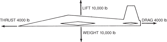
Figure 6.1 Aircraft in equilibrium flight.
Chapter 6 and 7 show the construction and use of the performance curves for thrust‐producing aircraft. Power‐producing aircraft (propeller‐driven aircraft) are discussed in Chapters 8 and 9.
THRUST‐PRODUCING AIRCRAFT
Some aircraft produce thrust directly from the engines; turbojet, ramjet, and rocket‐driven aircraft are examples of thrust producers. Of course, this thrust must be generated to overcome the drag of the airplane, or in the case of a rocket the weight (mass x acceleration of gravity). As a mass of gas is accelerated, thrust is generated possessing both magnitude and direction. Depending on the mass that is accelerated, and the velocity difference between the entrance and exit velocities of the jet engine, the magnitude of the thrust will vary. The efficiency of this process will affect fuel consumption as well as several important flight requirements. Fuel consumption is roughly proportional to the thrust output of these aircraft and, because range and endurance performance are functions of fuel consumption, the thrust required is of prime interest and will be the focus of our discussion.
A turbojet engine is a turbine engine that works by compressing subsonic air, then mixing the fuel with the compressed air in the combustion chamber, and after burning the mixture passes the hot, high‐pressure air through a turbine to drive the compressor and discharge from the exit nozzle at the highest possible velocity (Fig. 6.2). Thrust is produced when kinetic energy is created from the internal energy of the burning gases.

Figure 6.2 Turbojet engine.
U.S. Department of Transportation Federal Aviation Administration, Airplane Flying Handbook, 2004
A turbofan engine is a turbine engine that is very similar to a turbojet, but differs from a turbojet in that it contains an additional component, a bypass fan. Powered by the turbine section of the engine, the fan accelerates some of the intake flow of air around the combustion chamber and out the nozzle mixing with the hot, exhaust gases (Fig. 6.3). The bypassed air creates a more efficient thrust then the exhaust gas thrust due to the greater mass of the air that is being moved. Though the form drag of the greater intake area of the turbofan engine contributes to more parasite drag, the more efficient engine at subsonic speed has become a common engine design on Part 121 transport category equipment.
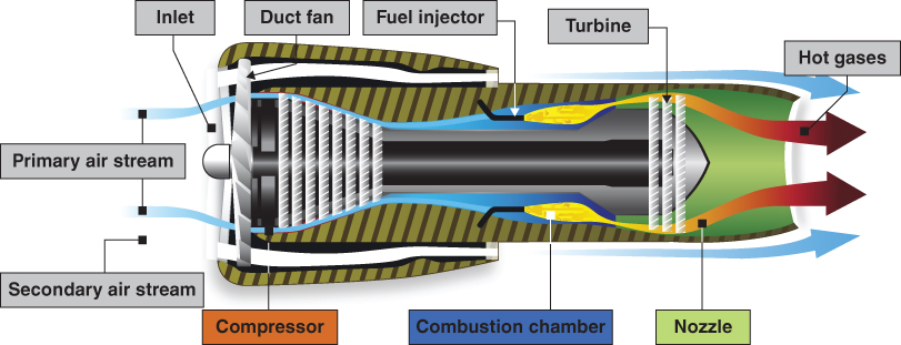
Figure 6.3 Turbofan engine.
U.S. Department of Transportation Federal Aviation Administration, Pilot's Handbook of Aeronautical Knowledge, 2008
Thrust‐Required Curve
Each pound of drag requires a pound of thrust to offset it; this is a very important consideration when depicting thrust using a graph. In Chapter 5 we discussed how the drag curve for an aircraft is drawn. We can now call this same curve a thrust‐required curve, or the minimum thrust required to maintain the aircraft in level flight. The curves used to illustrate the drag or thrust‐required (Tr) curves in this chapter are for the T‐38 supersonic turbojet trainer that is still in use today. Because this aircraft encounters a large amount of compressibility drag at high speeds, a sharp increase in the thrust required will be noted in this region.
Figure 6.4 shows the drag curve for the T‐38. The drag curve shows the amount of drag of the aircraft at various airspeeds. Figure 6.4 shows that the aircraft has a drag of 2000 lb at the buffet limit (stall speed), which is close to 160 knots, and at about 485 knots the drag is also 2000 lb. Minimum drag occurs at  , the bottom of the thrust‐required curve, which is at 240 knots velocity for aircraft of this weight, and has a value of 830 lb. As mentioned above, the thrust required is equal to the drag at this speed. The curve shown in Fig. 6.5 is identical to the one shown in Fig. 6.4, except the induced and parasite drag curves are omitted and the vertical scale is relabeled as “thrust required.” The curves in Figs. 6.4 and 6.5 are drawn for a 10,000‐lb airplane in the clean configuration at sea level on a standard day.
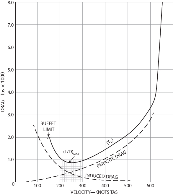
Figure 6.4 T‐38 drag curve.
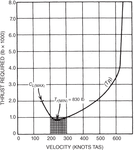
Figure 6.5 T‐38 thrust required.
PRINCIPLES OF PROPULSION
All aircraft power plants have certain common principles, based on Newton's second and third laws. You will recall that the second law can be written as  . Simply stated, an unbalanced force F acting on a mass m will accelerate a the mass in the direction of the force. The force is provided by the expansion of the burning gases in the engine. The mass is the mass of the air passing through the jet engine or through the propeller/rotor system. Thrust is directly proportional to density; as the density increases then so will the available thrust. The acceleration is the change in the velocity of the intake air per unit of time.
Newton's third law states that for every action force, there is an equal and opposite reaction force. This reaction force provides the thrust, T, to propel the aircraft:
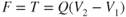
where
| T | = | thrust (lb) |
| Q | = | 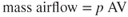 (Eq. 2.10) (slugs/sec) (Eq. 2.10) (slugs/sec) |
| V1 | = | inlet (flight) velocity (fps) |
| V2 | = | exit velocity (fps) |
Figure 6.6 shows a schematic of the process of producing thrust in a jet‐type engine. Ta represents thrust available.

Figure 6.6 Engine thrust schematic.
Equation 6.1 means that the thrust output of an engine can be increased by either (1) increasing the mass airflow or (2) increasing the exit velocity/flight velocity ( ) ratio. The first alternative requires that the cross‐sectional area of the engine be increased to allow more air to be processed. The second alternative requires increasing the relative velocity,
  . This imparts higher kinetic energy to the gases. The kinetic energy is wasted in the exhaust airstream, resulting in decreased efficiency of the engine.
Propulsion efficiency, ηp, can be expressed by

As V2 increases, propulsion efficiency goes down. This is shown in Fig. 6.7.

Figure 6.7 Propulsion efficiency.
Early turbojet engines were used on jet fighters. To keep the drag of the engines within reason, the engines could not have a large frontal area. This limited the amount of air that could be processed, and high exhaust velocities were required to obtain the needed thrust. As larger aircraft were developed, it was possible to use larger engines. Fanjet engines with large Q values improved the efficiency of jet engines, and now high‐bypass turbofans with large bypass ratios are much more fuel efficient than turbojets and even low‐bypass turbofans.
THRUST‐AVAILABLE TURBOJET AIRCRAFT
Turbojet aircraft engines are rated in terms of static thrust. The aircraft is restrained from moving, and the thrust is measured and converted to standard sea level conditions. It can be seen from the thrust Equation 6.1,  , that as the aircraft gains velocity, the mass flow increases, but the acceleration through the engine decreases (V2 is nearly constant). As we can see, if density increases then so will the thrust (Q is larger for the same intake area and V1).
The thrust available is nearly a constant with airspeed and is considered to be a constant in this discussion. Thrust varies, however, if the rpm of the engine is changed from the 100% value. The reduction of thrust is not linear with the reduction of rpm (Fig. 6.8). Thrust is also reduced with an increase in altitude. Equation 6.1 indicates that the mass flow decreases as the density of the air decreases. Temperature is also involved. Lower temperatures at altitude improve efficiency, so the loss in thrust is not as great as the decrease in density (Fig. 6.9).
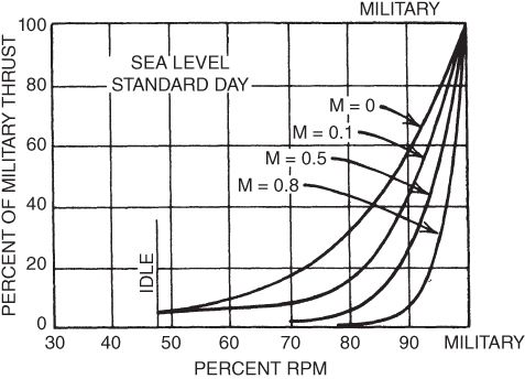
Figure 6.8 T‐38 installed thrust.
Figure 6.9 T‐38 thrust variation with altitude.
SPECIFIC FUEL CONSUMPTION
To move an aircraft through the air, a propulsion system must be used, and in this case our turbojet moves through the air as thrust is produced. In order to meet mission requirements, it can be imperative to understand the amount of fuel that is used to accomplish this process. Specific fuel consumption is an efficiency factor used to indicate the efficiency of an engine. Low values of ct, are desirable, and this is calculated by finding the fuel flow per pound of thrust developed by a jet engine:
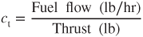
Turbojet engines are designed to operate at high rpm and will produce low specific fuel consumption values in this region. Figure 6.10 shows the variation of ct with rpm. The lowest values of ct occur between 95 and 100% rpm, and the increase in ct is very rapid as rpm is decreased. This does not mean you are consuming less fuel at higher levels of rpm, only that you are consuming less fuel per pound of thrust.
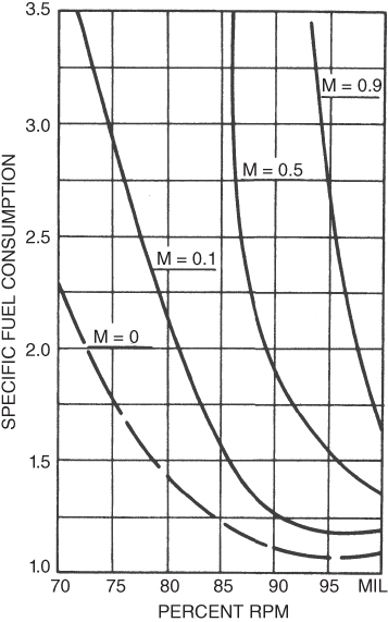
Figure 6.10 T‐38 ct–rpm.
The beneficial effect of lower temperature at altitude results in decreased specific fuel consumption (Fig. 6.11). Above the tropopause the temperature is constant, so no reduction in ct will occur. In fact, the compressor will not operate efficiently because the air density is reduced, causing an increase in ct.
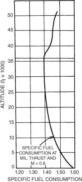
Figure 6.11 T‐38 ct–altitude.
FUEL FLOW
The total fuel flow, FF, equals the thrust of the engine, T, multiplied by the specific fuel consumption, ct; hence Equation 6.3 has been rearranged. As we can see in Equation 6.4, the greater the specific fuel consumption (or thrust for a given ct), the greater the fuel flow.

Thrust varies with rpm and altitude (Figs. 6.8 and 6.9). Specific fuel consumption varies with these same factors (Figs. 6.10 and 6.11). Fuel flow at altitude as a ratio of that at sea level, at a fixed rpm, is shown in Fig. 6.12.
Figure 6.12 T‐38 fuel flow–altitude.
THRUST‐AVAILABLE–THRUST‐REQUIRED CURVES
Performance depends on the relationship of the thrust‐available and thrust‐required curves. If the thrust available is equal to the thrust required, the aircraft can fly straight and level, but cannot climb or accelerate. An excess of Ta over Tr is required in order to accelerate, climb, or even turn the aircraft if maintaining level altitude is desired. The thrust‐available and thrust‐required curves are plotted for the T‐38 at 10,000 lb gross weight, clean configuration at sea level, in Fig. 6.13. The thrust available is plotted for two different conditions (100% rpm and 95% rpm) at sea level. The reduction of Ta with rpm was explained earlier (Fig. 6.8).
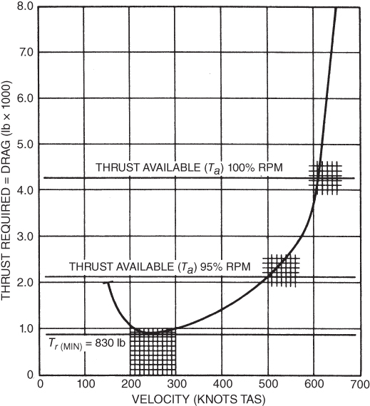
Figure 6.13 T‐38 thrust available–thrust required.
Figure 6.13 shows that a 5% reduction in rpm results in a reduction of Ta from 4200 lb to 2100 lb, close to a 50% reduction in thrust. This aircraft could not maintain altitude at any speed if the thrust is reduced below 830 lb as this is the minimum thrust required for the total drag in order to maintain level flight. This is a ratio of  of the Ta at 100% rpm, sea level conditions. Figure 6.8 shows that this occurs at about 88% rpm at sea level and Mach
  . Absolute ceiling occurs when Ta falls to 830 lb, indicating no excess thrust is available; Figure 6.9 shows that this occurs at about 47,500 ft.
ITEMS OF AIRCRAFT PERFORMANCE
Straight and Level Flight
When an aircraft is in steady (unaccelerated) level flight, it must be in equilibrium. Lift must be exactly equal to the weight of the aircraft, and the thrust on the aircraft must be exactly equal to the drag. The thrust is equal to the drag when the thrust available is equal to the thrust required. This happens when the Ta and Tr curves intersect. There are two possibilities for such an intersection. One is at the high‐speed region of flight and the other is at the low‐speed area. Our focus here will be on the intersection during the high‐speed region of flight; the problems in the low‐speed area will be discussed in a later chapter.
For nonafterburner flight the thrust available for the T‐38 is 4100 lb. From Fig. 6.13 it can be seen that the high‐speed intersection point of Ta and Tr is at 605 knots TAS, and if there is a reduction in rpm to 95% the value of Vmax decreases to 500 knots TAS.
Climb Performance
Every flight requires that the pilot climb the aircraft to some altitude. Mission requirements dictate the climb schedule. For instance, an intercept mission would require that altitude be gained as rapidly as possible, while a mission of long range would require that much distance be covered in the climb.
There are two basic types of climb: delayed climb and steady‐velocity climb. In a delayed climb the pilot builds up airspeed (kinetic energy) before starting to climb. The pilot then “zooms” the aircraft to altitude, which converts some of the kinetic energy to potential energy (height). This maneuver is used mostly by fighter aircraft pilots in intercept tactics, setting climb to altitude records, and other maneuvers.
Steady‐velocity climb is used much more often and exists in an equilibrium condition with all the forces along the flight path being balanced (Fig. 6.14). The forces acting along the flight path are thrust, T, and drag, D. Lift acts 90° to the flight path and the weight, W, acts toward the center of the earth. The climb angle is designated by the Greek letter gamma, γ. The weight vector is replaced by two other vectors. One is perpendicular to the flight path (W cos y) and the other is parallel to the flight path (W sin γ) and realistically acts at the aircraft's CG. For steady velocity the forces along the flight path must be balanced, and as we see thrust must now balance with the addition of the weight for a given climb angle plus the total drag. Thus,
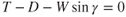
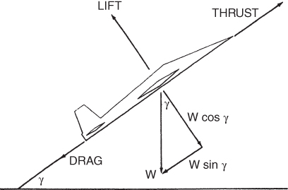
Figure 6.14 Forces acting on a climbing aircraft.
Angle of Climb
For the angle of climb, Eq. 6.5a is rewritten as
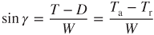
As an angle increases in size, the sine of the angle increases in value. The maximum climb angle will occur at the point where maximum thrust is at an excess  . For a turbojet, with the thrust available assumed to be constant with velocity, this will be where Tr (drag) is a minimum, which must be at
  (Fig. 6.15).
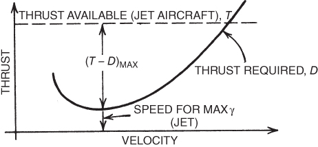
Figure 6.15 Velocity for maximum climb angle.
When an aircraft is in steady flight, horizontally, the lift is equal to the weight of the aircraft. Figure 6.14 shows that the lift is less than the weight if the aircraft is in a climb. This is possible because some of the thrust supports some of the weight of the aircraft. The steeper the climb is, the less the lift supports the weight. The extreme case occurs when the aircraft climbs straight up ( ). Then the lift would be zero and the thrust would support the entire weight of the aircraft and overcome the drag. A thrust/weight ratio of at least 1 is required for this maneuver. Obstacle clearance is affected by headwind and tailwind, as shown in Fig. 6.16. Once the airplane is airborne, the groundspeed is reduced by a headwind and increased by a tailwind. With reduced groundspeed, the time to reach the obstacle is increased, and more altitude is gained.
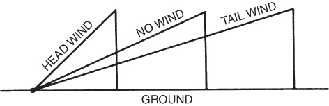
Figure 6.16 Wind effect on climb angle to the ground.
Rate of Climb
One other factor in obstacle clearance is the time required to reach the  velocity. After the jet takes off, it must accelerate to this velocity and, in doing so, precious ground distance is used up. Even though the jet is finally climbing at its highest climb angle, it may not clear the obstacle. The aircraft may clear the obstacle if the climb is started sooner, at a lower speed, and at a lesser climb angle (Fig. 6.17).
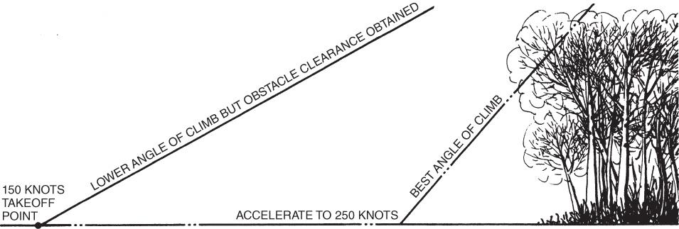
Figure 6.17 Obstacle clearance for jet takeoff.
The aircraft on the left in Fig. 6.18 is flying at maximum climb angle. The airspeed of this aircraft is relatively slow compared to the aircraft on the right. The aircraft on the right is flying at a smaller climb angle, but the much higher airspeed more than compensates for the lower angle, and it is at a higher altitude. The aircraft on the right has a higher rate of climb, ROC. This is shown in Fig. 6.19.

Figure 6.18 Climb angle and rate of climb.
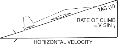
Figure 6.19 Rate of climb velocity vector.
We can solve the right triangle in Fig. 6.19 for the rate of climb:
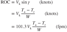
The velocity for maximum rate of climb cannot be determined by a simple examination of the  curves. Equation 6.6 shows that ROC depends on velocity and excess thrust, both of which are variables. However, by selecting various airspeeds and finding the corresponding values of Ta and Tr from Fig. 6.13, then solving Eq. 6.6, a plot of ROC versus velocity can be made similar to Fig. 6.20 and the velocity for maximum ROC can be found.
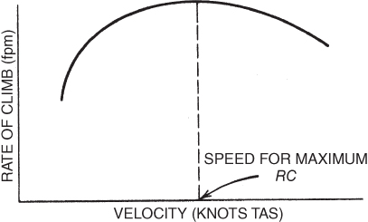
Figure 6.20 Velocity for maximum rate of climb.
Endurance
The endurance of an aircraft is the amount of time that it can remain airborne, and is independent of distance covered. It is useful when holding due to weather, air traffic, and so on, or to extend the time available for alternate airport diversions and to troubleshoot an emergencies. Since endurance is a function of fuel consumption, it is inversely proportional to fuel flow; thus long endurance times result from low fuel flow.
Figure 6.21 shows the thrust‐required curve for the T‐38 with the fuel flow also plotted on the vertical scale; note that Tr is 830 lb. The minimum fuel flow occurs at the point of minimum thrust required, which is the minimum drag point of the curve, so  . As a function of minimum fuel flow, maximum endurance for a jet aircraft occurs at
  .
.
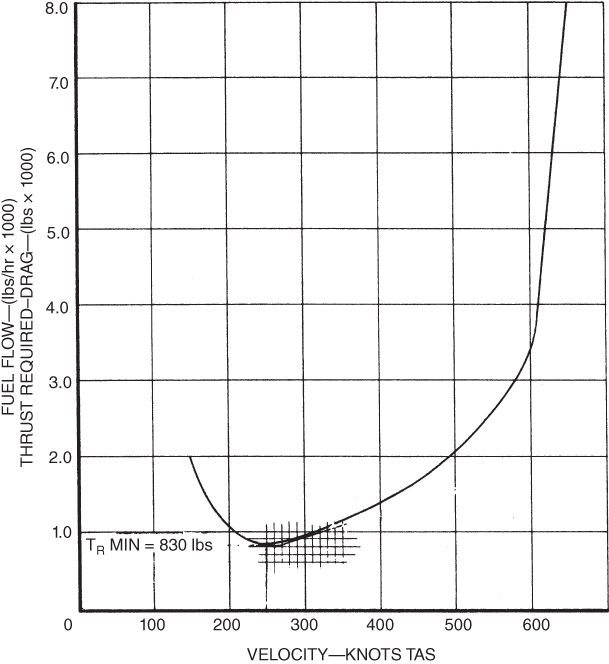
Figure 6.21 Finding maximum endurance velocity.
Specific Range
To get maximum range, an aircraft must fly the maximum distance with the fuel available, so we are looking for the maximum speed per fuel flow. Specific range can be defined by the following relationship:
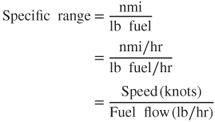
which means that
Graphically, the maximum specific range point can be shown on a fuel flow versus velocity curve, such as that in Fig. 6.22. Select any point on the Tr curve, such as A. Draw a straight line from A to the origin and drop a vertical line from A to the velocity scale. Label the angle at the origin of the resulting right triangle, angle θ1. The tangent of θ1, equals the opposite side of the triangle divided by the adjacent side. The opposite side is a measure of the fuel flow, and the adjacent side of the triangle is the aircraft's velocity:


Figure 6.22 Finding the maximum specific range velocity.
Hence, if FF/V is a minimum, tan θ must be a minimum, which means that θ must be a minimum. Only one point on the curve meets this requirement—the point where the line from the origin is tangent to the Tr curve at point B. θ2 is a minimum at B, and maximum specific range will occur if the aircraft is flown at this velocity, ∼300 kts. Maximum specific range occurs at a velocity corresponding to the tangent point of a straight line drawn from the origin to the curve. This is not  , but is the point where
  is a maximum.
Wind Effect on Specific Range
An aircraft flying into a headwind is in an unfavorable environment and thus should fly at higher true airspeed to reduce the effect of the headwind. Likewise, an aircraft flying with a tailwind is being helped on its way and thus should slow down to take advantage of the wind.
How much the airspeed should be altered is shown in Fig. 6.23. This illustration shows the correct airspeed for maximum range with a 100‐knot headwind or tailwind. To find the corrected airspeed for a 100‐knot headwind, plot the headwind on the velocity scale to the right of the origin. Use this point as a new origin and draw a tangent line to the curve. This will give the new airspeed for best range. In the example the no‐wind airspeed for maximum range was 300 knots and the corrected airspeed is 320 knots.
Figure 6.23 Wind effect on specific range.
Correcting for a tailwind is done similarly. The tailwind is plotted on the velocity scale, but to the left of the origin. A new tangent line will show the correct airspeed of 290 knots.
Total Range
The total range of an aircraft depends on the fuel available and the specific range. Specific range is a variable, and is affected by the gross weight of the aircraft, altitude, aircraft configuration, and pilot technique. As the weight of an aircraft decreases with fuel consumption, the specific range improves. We will see in the next chapter how velocity must be adjusted as weight changes in order to maintain maximum range. This variation is shown in Fig. 6.24. The total range is measured by the area under the curve, between the beginning and ending cruise weights. A way of approximating the total range is to find the average specific range and multiply it by the fuel burned.
Figure 6.24 Total range calculation.
Summary
For jet aircraft, we have seen that the following items of performance occur at (L/D)max:
- Minimum drag
- Maximum engine‐out glide range
- Maximum climb angle
- Maximum endurance
It is extremely important to know the airspeed or AOA for  for your aircraft. The airspeed will vary with aircraft weight, but AOA will not. With respect to altitude, indicated airspeed for
  will not change.
SYMBOLS
| ct | Specific fuel consumption (lb fuel/hr per lb thrust) |
| FF | Fuel flow (lb/hr) |
| Q | Mass airflow (slugs/sec) |
| ROC | Rate of climb (fpm) |
| SR | Specific range (nmi/lb fuel) |
| Ta | Thrust available (lb) |
| Tr | Thrust required |
| V1 | Intake (flight) velocity (fps) |
| V2 | Exit velocity |
| γ (gamma) | Climb angle (degrees) |
| ηp (eta) | Propulsion efficiency (%/100) |
EQUATIONS
- 6.1

- 6.2

- 6.3
- 6.4

- 6.5a

- 6.5b

- 6.6
PROBLEMS
- The equation
 shows that
- you can get more thrust from a jet engine by using water injection.
- you can get more thrust from a jet engine by decreasing the exhaust pipe area.
- Neither (a) nor (b)
- Both (a) and (b)
- Q in
 is the mass flow (slugs/sec). The mass flow depends on
- the cross‐sectional area of the turbojet engine inlet.
- the engine inlet velocity.
- the density of the air at the same point.
- All of the above
- The equation
 shows that decreasing the exhaust pipe area will
- decrease the propulsive efficiency of a jet engine.
- increase the propulsive efficiency.
- increase the thrust of the engine.
- decrease the thrust of the engine.
- Specific fuel consumption of a turbine engine at 35,000 ft altitude compared to that at sea level is
- less.
- more.
- the same.
- The thrust available from a jet engine at 35,000 ft altitude compared to that at sea level is
- less.
- more.
- the same.
- Fuel flow for a jet at 100% rpm at altitude compared to that at sea level is
- less.
- more.
- the same.
- A pilot is flying an airplane at the speed for best range under no wind conditions. A tailwind is encountered. To get best range now the pilot must
- speed up by an amount less than the wind speed.
- slow down by an amount equal to the wind speed.
- slow down by an amount more than the wind speed.
- slow down by an amount less than the wind speed.
- To obtain maximum range a jet airplane must be flown at
- a speed less than that for
 .
. - a speed equal to that for
 .
. - a speed greater than that for
 .
.
- a speed less than that for
- Maximum rate of climb for a jet airplane occurs at
- a speed less than that for
 .
. - a speed equal to that for
 .
. - a speed greater than that for
 .
.
- a speed less than that for
- Maximum climb angle for a jet aircraft occurs at
- a speed less than that for
 .
. - a speed equal to that for
 .
. - a speed greater than that for
 .
.
- a speed less than that for
- A single engine turbojet aircraft is flying at 296 knots TAS at sea level. The mass flow rate through the engine is 10 slugs/sec. The exit velocity from the engine is 800 fps. Find:
- The thrust of the engine
- The propulsive efficiency
- A jet airplane has thrust available as shown in Fig. 6.13 and specific fuel consumption as shown in Fig. 6.10. Find the fuel flow at sea level (military rpm and
 ).
). - Using Fig. 6.12, find the fuel flow for the airplane in Problem 12 at the tropopause.
- A jet airplane has the
 curves shown in Fig. 6.13. The airplane data are gross weight
  , standard sea level day, and clean configuration. Find:
- Vmax at 95% rpm
- V for maximum climb angle
- Sine of maximum climb angle
- Rate of climb at 400 knots
- V for best endurance
- V for maximum range
- V for maximum range with 100 knots of headwind