Neural Decoding II
Continuous Variables
Pascal Wallisch
In this chapter, you will look at how to decode a continuous, time-varying stimulus from neuronal signals. Specifically, this chapter will address how to decode the instantaneous hand position from a population of motor cortical neurons recorded from a macaque monkey. You will also see how information about how the hand position changes over time can be used to improve your decoding.
Keywords
kinematic; mean spike count; Bayesian statistics; maximum a posteriori estimation; recursive Bayesian estimation; state equation; observation equation
22.1 Goals of This Chapter
The preceding chapter explored methods of decoding movement direction from neuronal signals. The movement direction was a discrete stimulus, taking on one of eight possible values. In this chapter, you will look at how to decode a continuous, time-varying stimulus from neuronal signals. Specifically, this chapter will address how to decode the instantaneous hand position from a population of motor cortical neurons recorded from a macaque monkey. You will also see how information about how the hand position changes over time can be used to improve your decoding.
Note that this chapter assumes completion of Chapter 17, “Neural Data Analysis I: Encoding,” Chapter 18, “Neural Data Analysis II: Binned Spike Data,” and Chapter 21, “Neural Decoding I: Discrete Variables.”
22.2 Background
We previously discussed how neurons in the motor cortex carry information about upcoming movements. In the last chapter, you were able to use this information to decode the direction of a movement made to one of eight targets. But what do you do if movement isn’t so constrained as it is in the center-out task? Another common experimental paradigm in motor control literature can be described as the “pinball” task: a target appears somewhere in a 2D playing field, and as soon as the participant moves the cursor within this target, a new target appears at a different, randomly selected position. There are no hold times in this task, unlike the center-out task, so the hand is constantly moving. You are interested in decoding the trajectory of the hand, meaning you want to know X- and Y-positions of the hand at each time point. X- and Y-positions are examples of kinematic variables, meaning they describe the motion of the object (the hand), but not the forces that generated the motion. Considering just the limb kinematics is easier than considering the full limb dynamics, which requires a model of how muscle forces and the physical properties of the limb interact to produce motion.
What method can you use to decode these kinematic variables? You could just modify the algorithms you have already seen. Recall that the population vector has a magnitude as well as direction. If you assume this magnitude is proportional to the instantaneous speed, you could simply compute a population vector for each time bin and then add them tail to tip to create an estimate of the trajectory. This was, in fact, an early approach to the problem (Georgopoulos, 1988).
In this chapter we will take a couple of different approaches. We mentioned previously that a simple neuronal encoding model assumes the firing rate varies linearly with stimulus intensity. You can apply this to motor cortical neurons and assume they fire linearly with the instantaneous hand position. For decoding, you simply invert this equation and derive an estimate of hand position using a linear function of firing rates. Another approach is to divide the X- and Y-axes into a grid and then use the same maximum likelihood method we used for center-out data to determine which grid square the hand is located in. As you will see, the fact that the hand position varies smoothly as a function of time introduces some new wrinkles.
Load the dataset for this chapter, available on the companion web site (data courtesy of the Hatsopoulos laboratory). There are two main variables: kin stores the X- and Y-positions (sampled every 70 ms), and rate stores the number of spikes in each 70 ms bin. Now look at the relationship between just one kinematic variable (Y-position) and one neuron’s spike count. Notice how the indices are offset to create a vector of spike counts that lead the kinematics by two time bins (or 140 ms):
| lag=2; | %Lag between neural firing and hand position |
| y=kin(lag+1:end,2); | %Y-position of the hand |
| s=rate(1:end-lag,36); | %Corresponding spike count of one neuron |
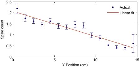
We are interested in how the spike count varies as a function of hand position (for simplicity, right now we only focus on position in the Y-direction). However, if you were to plot the position versus the raw spike count as a scatter plot, the result would be confusing, because the spike counts are highly variable. It is better to look at how the mean spike count varies as a function of position. To do this, we will divide the position variable into 15 1-cm wide bins, and average the corresponding spike counts. We will also keep track of the standard deviation, so we can compute a standard error: this is equal to the standard deviation divided by the square root of the number of data points. We can then plot a confidence interval for the empirical mean, as the “true” mean should fall within two standard errors of empirical mean 95% of the time. The error bars corresponding to a confidence interval can be plotted using the MATLAB® function errorbar.
The following code uses that function to plot the mean spike count as a function of the position of the hand:
| yEdge=[0:15]; | %Bin edges |
| for ii=1:length(yEdge)-1 | |
| ind=find(y>yEdge(ii) & y<=yEdge(ii+1)); | %Find positions within bin |
| meanS(ii)=mean(s(ind)); | %Mean of spike counts for this bin |
| stdS(ii)=std(s(ind)); | %Standard deviation |
| errS(ii)=stdS(ii)/sqrt(length(ind)); | %Standard error |
| end | |
| yCenter=yEdge(1:end-1)+.5; | %Center of each bin |
| errorbar(yCenter,meanS,2*errS,’.’) | %Plot mean with error bars |
In this case, the mean spike count seems to vary roughly linearly with the position. If you fit the spike counts as a linear function of position using polyfit (see Chapter 17) and plot the fit, you will end with something like Figure 22.1.
22.2.1 Linear Filter
You now have a decoder relating one neuron’s spike counts S to the instantaneous y-position Y, which takes the familiar linear form, Y=mS+b, where m and b are the coefficients returned by polyfit. But what exactly is the MATLAB software doing when you run polyfit? It is determining the optimal linear regression that minimizes the squared residuals (which are the differences between the fitted data and the actual data). The optimal linear regression can be expressed analytically. If you express the linear relationship in matrix form as Y=Sf, where Y is the kinematics, S is the spike counts, and f is the decoding filter (the y-intercept b has disappeared, but you will add a column of 1s to S to account for this), then minimizing the squared residuals is the same as solving the following equation:
 (22.1)
You can use this to solve for the desired decoder:
 (22.2)
A matrix inverse can be computed in MATLAB with the function inv, and a transpose is denoted with an apostrophe. Compare this solution to the values you derived with polyfit:
| p=polyfit(s,y,1) | %Linear regression |
| s=[s ones(length(s),1)]; | %Add a row of 1’s to allow y-intercept |
| f=inv(s’*s)*s’*y | %Analytical linear regression |
The advantage of this approach is that you can easily add more neurons or more kinematics to the model: you just add more columns to S and Y. The following code shows how to fit a linear filter to the training data for this dataset, using all of the kinematics and all the neuronal firing rates lagged two time bins (140 ms):
| numBin=length(kin); | %Number of datapoints |
| yTrain=kin(lag+1:numBin,:); | %Kinematic training data |
| sTrain=rate(1:numBin-lag,:); | %Neural training data |
| sTrain=[sTrain ones(numBin-lag,1)]; | %Add vector of ones for baseline |
| f=inv(sTrain’*sTrain)*sTrain’*yTrain; | %Create linear filter |
Once you fit the linear filter to the training data, load the test data and use the following code to see how well the decoder performs (remember, you always want to test on different data than you trained with to prevent over-fitting):
| numBin=length(kin); | |
| sTest=[rate(1:numBin-lag,:) ones(numBin-lag,1)]; | %Test neural data |
| yActual=kin(lag+1:numBin,:); | %Actual test kinematics |
| yFit= sTest*f; | %Predicted test kinematics |
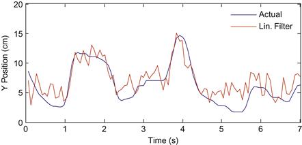
If you plot the actual Y-position versus the estimated position, the linear filter seems to be doing a pretty good job (Figure 22.2). This approach of using a linear filter as a decoder was used in 2002 to show that a macaque monkey could successfully control a computer cursor with neuronal signals (Serruya et al., 2002) and again in 2006 to show that a human with tetraplegia could control a variety of neural prosthetics with neuronal signals (Hochberg et al., 2006). Of course, the linear filter can be used on data recorded outside the motor cortex. For example, it has been used to decode visual information from retinal ganglion cells (Warland et al., 1997).
22.2.2 Maximum a Posteriori (MAP) Estimation
We just saw that a linear filter can be used to generate a continuous estimate of the position of the hand from neural data. This is different, though, than what we did in Chapter 21, where we computed the probability of the neural data given each movement direction and picked the direction which corresponded to the most likely data. Can we use that approach here? Yes; however we will simplify the problem by approximating the continuous estimate with a discrete one, by binning the hand position. Since the targets were 1 cm square, we can try to decode the position at a 1 cm resolution. How do we do that?
First, we need a prediction of the neural firing rate. In Chapter 18, we introduced log-linear models, which can be fit with generalized linear model techniques using the function glmfit. This has the advantage of always predicting a non-negative firing rate. We will use that here to fit an encoding model relating the Y-position to neural firing (recall that we assumed fixed lag of 2 time bins, or 140 ms). We can then use this model to predict the firing rate of each neuron at one of 15 evenly spaced Y-positions which cover the playing field.
| yCenter=[0.5:1:14.5]; | %Discrete set of positions |
| numNeuron=size(rate,2); | %Number of neurons |
| for n=1:numNeuron | %Loop over all neurons |
| coeff(n,:)=glmfit(yTrain(:,2),sTrain(:,n),’poisson’); | %Fit the encoding model |
| sFit(n,:)=exp(coeff(n,1)+coeff(n,2)*yCenter); | %Predict firing rate |
| end |
We already assumed that the neuronal firing rates are Poisson distributed for the encoding model. If we assume all neurons are conditionally independent, then the probability of a vector of spike counts is just the product of the probabilities of each spike count given our prediction (see Equation 21.4). We mentioned in Chapter 21 that it is sometimes advantageous to work with the sum of the logs of probabilities instead of the product of the probabilities, but it doesn’t turn out to be an issue with this data. What this gives us is the conditional probability (discussed in Chapter 20) of observing a vector of spike counts S given we are at position Y: P(S|Y).
| for t=1:length(sTest) | %Loop over all trials |
| frTemp=sTest(t,1:numNeuron); | %Select spike counts for one time bin |
| prob=poisspdf(repmat(frTemp’,1,15),sFit); | %Prob. of each count given position |
| probSgivenY(t,:)=prod(prob); | %Prob. of all counts given position |
| end |
We aren’t done yet, though, because this isn’t actually the probability we are interested in. Rather, we want the conditional probability of the position Y given the observed spike counts S: P(Y|S). This is more useful, because to decode position, we just select the position Y with the highest probability. But how do we convert from one to the other? Recall from Chapter 20 that conditional distributions can be written in terms of a joint distribution: P(S|Y)=P(S,Y)/P(Y) and P(Y|S)=P(S,Y)/P(S). We can make a simple substitution to come up with an expression known as Bayes’ rule:
 (22.3)
When people talk about Bayes’ rule or Bayesian statistics, they often talk about prior and posterior distributions. In the context of this decoding problem, the prior distribution is P(Y). That is, the prior represents whatever prior knowledge we have about the position of the hand, before we see the neural spike counts. We then use Bayes’ rule to incorporate this prior with the information we get from neural data. The result of this combination is P(Y|S), called the posterior distribution. This represents all of our knowledge of the position of the hand after we get to see the neural firing rates.
What prior information do we have? To start with, we can just look at how long the cursor dwells near one of the 15 discrete positions, and compute a histogram. If we then normalize the histogram to sum to 1, that gives us P(Y). Now, the expression above also contains P(S), but it turns out we don’t actually have to calculate this, because we don’t care about what the probability of a given position actually is, we just want to know which position is most probable. This strategy is known as maximum a posteriori (MAP) estimation. “A posteriori” is just the Latin name for knowledge possessed after making an observation (in this case, of neural spike counts), whereas “a priori” refers to knowledge possessed before making an observation. The MAP estimate of the position is shown below (the hat over the Y indicates it is an estimate of position and not the actual value Y):
 (22.4)
The code below determines the prior distribution P(Y) and the MAP estimate of the position:
| probY=histc(yTrain(:,2),[0:15]); | %Histrogram of position values |
| probY=probY(1:15)/sum(probY(1:15)); | %Convert to a probability |
| for t=1:length(sTest) | |
| probYgivenS(t,:)=probSgivenY(t,:).*probY’; | %P(Y|S) is proportional to P(S|Y)P(Y) |
| [temp maxInd]=max(probYgivenS(t,:)); | %Find index of maximum |
| mapS(t)=yCenter(maxInd); | %Find position with highest P(S|Y) |
| end |
The results of the MAP decoding are shown in Figure 22.3 for the first few seconds.
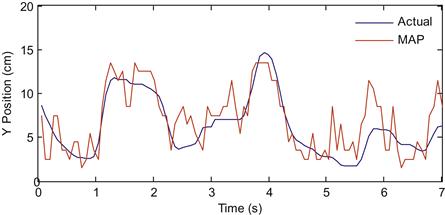
Figure 22.3 The actual Y-position of the hand (blue) compared to the reconstruction using maximum a posteriori (MAP) estimation (red).
While the MAP estimate does okay, it is a little disappointing that it appears to do worse than a linear filter, but takes more effort to compute. How can we improve on this algorithm?
22.2.3 Recursive Bayesian Estimation
Our MAP estimate contained two components: P(S|Y) and P(Y). The first expression, P(S|Y), is called the observation equation, because it details the probability of observing a given set of spike counts S given the position at Y. This is the same as the encoding models we developed in Chapter 18. But what about the prior distribution, P(Y)? If you actually look at values for the variable “probY,” computed above, you’ll see that all it says is that the hand is more likely to be in the middle of the playing field than at an edge. That’s not a lot in terms of prior information. An alternative way to determine the prior distribution for Bayes’ rule is to use a state equation, which describes how the position of the hand evolves as a function of time. The hand can only move so much during a 70 time bin, so we will make the assumption that the position of the hand in the next time bin yt+1 is a function of the hand in the current time bin Yt, plus some error term et+1 (which in this case is the hand’s velocity).
 (22.5)
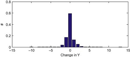
So what kind of distribution can we define for this error term? We can look at this by simply differentiating the position for our training data, and looking at what kind of values we see. Since the Y-position is more or less between 0 and 15 cm, the error term should be between −15 and +15 cm/bin. So we will compute a histogram of the observed errors between the position terms for each time bin.
| yDiff=diff(yTrain(:,2)); | %Compute error term |
| yDiffEdge=[-15.5:15.5]; | %Define edges |
| yHist=histc(yDiff,yDiffEdge); | %Compute histogram |
| probDiffY=yHist(1:31)/sum(yHist); | %Convert to probability |
| bar([-15:15],probDiffY); | %Plot probability |
Your output should look like Figure 22.4.
What is interesting about this figure is how tightly clustered it is around zero. In fact, over 97% of the bins have an absolute change in position of less than 2.5 cm. So the position doesn’t change that quickly as a function of time. This means that if we have a good estimate of where the position is in the current time bin, we also have a pretty good estimate of where it will be in the next time bin. How do we actually calculate the probability of cursor position of the next time bin if we know the probability of the current time bin? We just have to add up all the different combinations which could lead to a given position. For example, if I know the probability of being at each position now, what is the probability of being at 5 cm one time step from now? We just need to sum the probabilities of all combinations which add up to 5: start at 5 and stay there, start at 6 and move down one, start at 4 and move up one, etc. This kind of procedure is known as convolution, which we touched on in Chapters 16 and 20. Basically, we just need to take the probability distribution of the position at the last time point, and “blur” it by how much we think the position can shift in one time step. The probability of the current position at location j can be written:
 (22.6)
In MATLAB, we could use a loop to evaluate this expression, but it is faster to use the built-in function conv. We can use this probability distribution as an alternative form of the prior information about position at the current time point t: P(Yt). We generate this prior information from our previous best estimate of the position at the last time point t−1: P(Yt−1). This is what is meant by recursive Bayesian estimation; the estimate of the current time point is based on an estimate of the last time point to create prior information, which is incorporated with neural data using Bayes’ rule. Given Bayes’ rule, we can describe the probability of the current position Yt given all the neural observations up to the current time point S1:t as the following:
 (22.7)
We’re going to make a few assumptions to simplify things. First, we assume that the current position only affects the current neural observation (or rather, the neural observation at a specific lag), which means we can replace  with
with  . Second, for the expression
  we will make use of the state equation, which assumes that the position at the current time is a function of the position of the last time point. However, we don’t know the exact position at the last time point, but we will assume that we have probability distribution of the position given past neural observations:
  . We can convolve this expression with the velocity term in our state equation,
  , to come up with a prior distribution of position for the current time point:
  . Finally, we will ignore the normalizing factor
  , and look at a proportionality (designated with an “
 ”) instead of an equality. Because we are dealing with a discrete set of positions, we can normalize by forcing the probabilities to sum to 1. Thus, we can combine these assumptions to come up with the following expression for our a posteriori (after we see the neural observations) estimate of position:
 (22.8)
The expression for our a priori (before we see neural data) knowledge,  , is found by convolving the last estimate,
  , with the error term (Et) in our state equation, as we did earlier:
 (22.9)
There is one curious thing about this expression—we always reference the last estimate  . But what do we do on the first time step? Well, it turns out we just need to make a guess, and the estimate will converge to a better estimate over a few time steps. For simplicity, we can assume a uniform distribution over our 15 possible positions for the first time step:
  . We then convolve this with the error distribution we determined earlier. In MATLAB, we can do this with the following code:

However, when we convolve, this actual gives use a distribution of positions from −14 cm to 30 cm. We are assuming the position can only be between 0.5 and 14.5 cm, so we trim out the middle portion of the distribution, and re-normalize so the probabilities sum to one.
This gives us the prior estimate of position. To get the posterior estimate, we just need to multiply (element by element) this prior distribution with the probability of the neural data S given the position Y, which we already computed for the MAP decoder. Again, we will normalize to make the probabilities sum to 1. Finally, instead of picking the most likely position, our estimate will be a probability-weighted sum of the possible positions.
| probPostY(1,:)=probPriorY(1,:).*probYgivenS(1,:); | %Combine prior with neural data |
| probPostY(1,:)=probPostY(1,:)/sum(probPostY(1,:)); | %Normalize probabilities |
| bayesY(1)=sum(probPostY(1,:).*yCenter); | %Bayesian estimate of position |
That’s just the first time point, though. For the rest of the time points, we do the exact same thing, but we proceed recursively, always building off of our previous estimate.
%Convolve last estimate with error term for prior
probTemp=conv(probPostY(t-1,:),probDiffY);
probPriorY(t,:)=probTemp(16:30)/sum(probTemp(16:30));
%Combine prior with neural data for the posterior
probPostY(t,:)=probPriorY(t,:).*probYgivenS(t,:);
probPostY(t,:)=probPostY(t,:)/sum(probPostY(t,:));
%Convert distribution to a single estimate of position
If you compare the recursive Bayesian estimate to the actual position, your results should look similar to those shown in Figure 22.5. Notice how the estimate is much less jerky than the MAP estimate or the linear filter, because we enforce continuity of the position trace with our state equation.
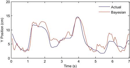
Figure 22.5 The actual Y-position of the hand (blue) compared to the reconstruction using recursive Bayesian estimation (red).
There are some caveats to this comparison. First, the linear filter doesn’t traditionally make use of just one time bin’s worth of data. Instead, the linear filter can make use of all neural data going back as much as a second. This averages out some of the noise inherent in measuring spike counts, so the position estimate becomes much smoother. You will look at the effect of adding more neural data to the linear filter in the exercises. Second, our recursive Bayesian decoder only looked at position tuning in the neural data, even though we know that neurons also encode velocity. You will also add velocity to the Bayesian decoder in the exercises.
One drawback of the discrete Bayesian decoder we present here is that the computational requirements increase quickly as you add more degrees of freedom. Here, we have 15 possible states for the Y-position. If we wanted to track X and Y concurrently, we would have 15^2=225 possible states, and tracking X and Y velocity would increase the state space even further. For this reason, real-time Bayesian decoding for brain machine interfaces often makes use of a Kalman filter (Wu et al., 2004), which provides a computationally efficient, closed-form solution to the decoding problem, if certain assumptions are made (linear observation and state equation; Gaussian noise). The advantage of discrete Bayesian decoding is that the observation and state equation can be changed to anything you want, so they can handle nonlinearities. You can explore that in the project for this chapter, where you will design and implement your own decoder.
22.4 Project
Create your own decoding algorithm. The simplest scenario would involve modifying the state or observation equations for the recursive Bayesian decoder. For example, perhaps neural firing is actually a non-linear function of the hand position or velocity (the function nlinfit might be useful). Or perhaps the current position is a function of more than just the previous position. You could also try your own techniques, as long as they are optimized solely from the training data. Comment on the assumptions that you are changing, and why you think this is an improvement. Report both the mean-squared error and the correlation coefficient of your fit for Y-position of the test data.
