25.1 ROUNDOFF AND TRUNCATION ERRORS
A computing machine is finite, both in size and speed; and, as you have seen, mathematics regularly uses the infinite, both (1) in the representation of numbers and (2) in processes such as differentiation, integration, and infinite series. When we try to carry out our mathematical operations on a machine, the finite size of the machine gives rise to roundoff\ and the finite processes used by the finite-speed machine give rise to truncation errors.
As an example of roundoff, consider the representation of the number one-third as a decimal in an eight-decimal-digit machine:
![]()
There is roundoff due to the dropped digits past the last retained digit. Thus, most numbers that arise during a computation will be rounded off. The effect of roundoff appears most seriously when two numbers of about the same size are subtracted; then, because the leading zeros are shifted off (in scientific work), the rounded digits move over into the more significant digit positions of the number.
Example 25.1-1
Due to roundoff effects, you can sometimes get spectacular results. Suppose that ![]() is so small that
is so small that ![]() 2 is less than 10–8. Then it follows that
2 is less than 10–8. Then it follows that
on an eight-decimal-place computer. Also, for a small number ![]() ,
,
(1 + ![]() ) – (1 –
) – (1 – ![]() ) = 2
) = 2![]()
At best the leading digits of this result are the first digits of ![]() , and there is a significant loss of relative accuracy.
, and there is a significant loss of relative accuracy.
Example 25.1-2
Consider
![]()
for large x. There will be a great deal of cancellation, but if you remember what you did when using the delta process for the function y(x) = ![]() you rearrange this in the form
you rearrange this in the form
![]()
which is easily evaluated without serious loss of accuracy.
The methods of rearranging a computation before evaluation to avoid serious loss of accuracy resemble, many times, the methods we used to rearrange an expression before taking the limit in the four-step ![]() process.
process.
Another tool that is sometimes useful in avoiding roundoff is the mean value theorem,
f(x + a) – f(x) = f′(θ)a
where θ is in the range x to x + a.
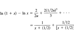
Example 25.1-3
Evaluate
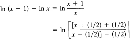
f(x) = ln (x + 1) – ln x
for large x. By the mean value theorem, we have that their difference is, for some θ in the interval 0 < θ < 1,
![]()
A reasonable choice of θ might be θ = 1/2. Hence we have, approximately,
![]()
Example 25.1-4
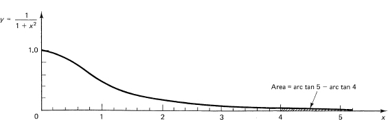
Evaluate, for large n (see Figure 25.1-1)
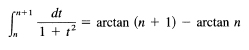
Figure 25.1-1
For large n, there will be a great deal of cancellation of the leading digits of the two numbers since both are near π/2. If we apply some trigonometry, we find that from the identity (16.1-16)
![]()
Taking the arctan of both sides gives
![]()
We now write θ = arctan a and ϕ = arctan b to get the identity we need:
![]()
Hence we have
![]()
which can be evaluated accurately, and furthermore involves only one arctan evaluation.
Rule. It is better to anticipate roundoff errors and rearrange the formulas than it is to try to force your way through stupid forms of writing and then evaluating the formulas. The claim that “double precision arithmetic is the answer to all roundoff problems on a computer” is only partly true. Often the methods in the calculus are necessary to handle the roundoff errors that arise.
A final tool from the calculus is the use of the power series representation of functions. The words “truncation error” come from the approximation of infinite series using only the leading terms, truncating the series. This is exactly what we did in the theory of infinite series. We studied the sequence of partial sums. In computing we are forced to settle for some finite sum, and we cannot take the limit. We will deal with this matter only slightly, as the serious theory is inappropriate for an elementary course.
We use Example 25.1-3 again.
Set x + 1/2 = u. We have the more symmetric form
![]()
But we have (set 1/2u = t)
![]()
and, using the power series expansions of the two logs, we get
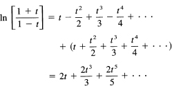
Using this expression, with t = 1/2u and u = x + 1/2, you get
and from the first term we have the same approximation as before (Exercise 25.1-3), but we now have some indication of the higher-degree correction terms in the approximation.
1. Evaluate for large x, ![]()
2. Evaluate for small x, (1 – cos x)/sin x.
3. Evaluate for large x, ![]()
4. Evaluate for large x, (1 + x)l/3 – x1/3.
5. For x near 4, evaluate ![]()
6. For x near zero, evaluate ![]()
7. For small x, evaluate (x – sin x)/(x – tan x).
8. Show that for small x, x{e(a+b)x – 1 }/{(eax – 1)(ebx – 1)} is approximately (a + b)/ab.
25.2 ANALYTIC SUBSTITUTION
Let us review how we handled past encounters with numerical methods. In Newton’s method, Section 9.7, we replace the curve locally with the tangent line that passes through the point and has the same slope as the curve whose zero we want. We replace an intractable function with one that we can handle (a straight line). We then simply find the zero of the straight line and use that as the next approximation to the zero of the function.
When we faced numerical integration (Section 11.11), for both the trapezoid and midpoint rules, we analytically substituted a local straight line for the given curve, the secant line in the trapezoid rule, and the tangent line at the midpoint of the interval in the midpoint rule. For Simpson’s rule (Section 11.12), we approximated the function over a double interval by a parabola and then integrated the parabola over the double interval as if it were the function (locally).
We immediately generalize and observe that we can make an analytic substitution of any function (that we can handle) for the given function (that we cannot handle), and then act as if it were the original function. The quality of the approximation is a matter that we will later look into briefly. Polynomials are widely used because they are generally easy to handle, but the Fourier functions, sin kx and cos kx, are increasingly being used. As you will see, the details of the derivation depend on the particular set of approximating functions you pick, but the form of the formula you derive is the same. Consequently, the amount of computing you will do when using the formula will be about the same (the formula will not directly involve the particular functions you use in the approximation process). The major tool will be the familiar method of undetermined coefficients.
We have used the method of undetermined coefficients several times to find local polynomials passing exactly through the data, and we have at times used polynomials to get a least squares fit. Thus, in setting out to create a formula to use in numerical methods you must decide:
1. What information (sample points, function, and/or derivative values) to use.
2. What class of approximating functions to use (polynomials, sines and cosines, or exponentials).
3. What criterion to use to select the specific function from the class you adopted (exact match at the given points, least squares, etc.).
4. Where you want to apply the criterion.
This last point is difficult to explain at the moment, but it may become slightly clearer as we go on.
We begin with the polynomial approximation of a function when we are given some data (samples) about the function. The samples may be at any place and involve the function as well as various values of derivatives. Although you tend to think that the derivative is usually messier than is the original function, when you ask about the computing time you find that, once you have the special functions (sin, cos, ![]() , In and exp), which arise in the original function, you also have most of the special functions that arise in the derivative; and it is the special functions that occupy most of the machine time on a computer even though each seems to be but one instruction. When you differentiate a function, no new awkward pieces arise, but a sine can give rise to a cosine, and conversely; generally, once you have paid the cost of evaluating the parts of a function, the cost of a derivative is cheap.
, In and exp), which arise in the original function, you also have most of the special functions that arise in the derivative; and it is the special functions that occupy most of the machine time on a computer even though each seems to be but one instruction. When you differentiate a function, no new awkward pieces arise, but a sine can give rise to a cosine, and conversely; generally, once you have paid the cost of evaluating the parts of a function, the cost of a derivative is cheap.
Example 25.3-1
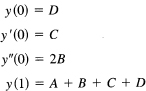
Suppose we want a polynomial that takes on the (general) values y(0), y(1), y´(0), and y´(1). With four conditions, we need four undetermined coefficients, a cubic:
![]()
The four conditions give rise to the four equations
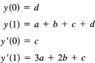
Eliminating c = y’ (0) and d = y (0), we get
![]()
These two equations are easily solved for a and b:
![]()
and we have the cubic through the given data.
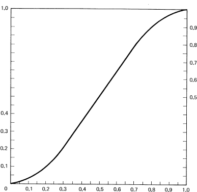
A specific, useful case occurs when y(0) = y´(0) = y´(1) = 0 and y(1) = 1 (see Figure 25.3-1). The coefficients are a = –2, b = 3, c = 0, and d = 0. The polynomial through the data is
y(x) = –2x3 + 3x2 = x2(3 – 2x)
It is easy to verify that this equation satisfies the given data.
Example 25.3-2
Suppose we use the general cubic polynomial (25.3-1) to analytically approximate a curve in the interval, and from this get an approximation to the integral (another integration formula)
Figure 25.3-1 y = x2(3-2x)
![]()
We integrate the approximating cubic of Example 25.3-1 to get
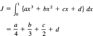
Direct substitution of the values of the coefficients produces the formula
![]()
This formula makes a very interesting composite integration formula for functions with continuous first derivatives, since it leads to
![]()
The two end derivatives are the only correction terms needed to gain the local accuracy of a cubic.
Suppose all you know about the function is y(0), y′(0), y″(0), and y(1), and you want the integral over the interval 0 to 1.
First you find the interpolating polynomial using undetermined coefficients:
y(x) = Ax3 + Bx2 + Cx + D
To get the formula, you impose the four conditions:
from which you get
![]()
and you have the interpolating polynoial.
To get the approximating integral, you integrate this polynomial:
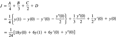
This is the approximation for the integral in terms of the given data.
1. Find the quadratic through (0, 1), (1, 2), (2, 3).
2. Find the quadratic through (–1, a), (0, b), (1, c).
3. Find the cubic through (0, 1), (1, 0), (2, 1), and (3, 0).
4. Using f(1/3) and f(2/3), find an integration formula of the form ∫01f(x) dx = af(1/3) + bf(2/3).
25.4 THE DIRECT METHOD
In all the preceding examples, the final formula was linear in the given data. If you think about the process, you see that this is inevitable; it is impossible that products or powers of the data will arise using the methods we have used (think about dimensional analysis). You know, therefore, that the form of the final answer is a linear expression in the given data. This suggests that by using the method of undetermined coefficients you can go directly to the final answer.
How can this be done? Since the interpolation formula is true for any data of the given form, the integration formula is also true for that data. In particular, the integration formula must be true for the particular functions y(x) = 1, x, x2,…. xm – 1, where m-1 is the highest power used in the interpolation formula. Conversely, since integration is a linear process, if the integration formula is true for the individual powers of x, then it must be true for any linear combination of the powers, for any polynomial of degree m – 1.
The plan is to set up the form with undetermined coefficients and then impose the conditions that the formula be exact for as many consecutive powers of x as there are coefficients, beginning with y(x) = 1, and going on to y(x) = x, y(x) = x2, … , as far as you can go.
Example 25.4-1
Derive by the direct method the integral in Example 25.3-2.
Given y(0), y(l), y′(0), and y′ (1), the form to choose is
![]()
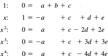
Next write out the equations for the conditions that the equation be exactly true for each power of x as indicated on the left. These are the defining equations:
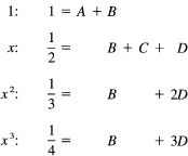
In the first line y = 1, so J = 1 and y(0) = 1, y(1) = 1, y′(0) = 0, and y′(1) = 0. Hence the A and B terms are present and the C and D terms are not. In the second line the integral of y(x) = x over the interval 0 to 1 is 1/2; y(0) = 0 for y = x, y(l) = 1, y′(0) = 1, and y′(l) = 1. Hence the B, C, and D are present, but the A is missing. Similarly, for the third line you use y (x) = x2 and for the fourth line you use y (x) = x3.
To solve these four equations, simply subtract the third from the fourth to get
![]()
Use that D in either of the bottom two equations, say the last one, and you have
![]()
From the top equation, you get immediately
![]()
Finally, from the second equation (the only one involving C)
![]()
and we have the same formula
![]()
as before, but with a great deal less labor!
Example 25.4-2
Given data for y(x) at x = –1,0, and 1, find an approximation for the integral
![]()
The form we use is
J = ay(-1) + by(0) + cy(1)
and we impose the three conditions that the formula be true for y = 1, for y = x and for y = x2. We need the integrals
![]()
For n = 0, it is an arcsine, and the value is π. For n = 1, the integrand is odd, so the integral is 0. For n = 2, the integral, when you use the substitution x = sin θ to get rid of the radical, becomes a Wallis integral with the value π/2 (remember both limits).
The defining equations are, therefore,
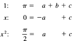
From the second equation, a = c, from the bottom equation, a = c = π/4, and from the top, b = π/2. Hence the formula is
![]()
This differs from Simpson’s formula by both (1) the front coefficient (now π/4 instead of 1/3), and (2) the middle coefficient is twice the end coefficients rather than four times as large. It shows the effect on the end coefficients due to the factor
in the integrand. Notice that we did not approximate the whole integrand by a polynomial, only the unknown function y(x).
Generalization 25.4-3
We see that given almost any data and any linear operation (integration, interpolation, and differentiation are examples of such operations), we can set up the defining equations that make the formula exactly true for f(x) = 1,x,x2, … , as far as there are arbitrary coefficients to be determined. We need to compute the moments of the linear operator, (typically, we have used integration with or without a weight factor and have at times used derivatives as well as function values). If the moments cannot be found analytically (in closed form), then you can find them numerically, once and for all, using some suitable formula such as Simpson’s, at a suitably small spacing. Once found, the moments are then the left-hand sides of the defining equations. The right-hand sides depend only on the given data locations; one side depends only on the form assumed and the other only on the formula being approximated. The solution of the linear equations determines the formula.
We see a further generalization: we did not have to use the powers of x as the criterion for exactness; we could use any set of linearly independent functions. In particular, we might use the first few terms of a Fourier expansion if that seemed suitable. The arithmetic to find the formula might be more difficult, but the arithmetic in the use of the formula would be the same; only the numerical values of the unknown coefficients would be different.
You are not restricted to integration formulas; the derivation of any linear formulas would go just about the same: find the “moments” of the operation on the left-hand side by some method, write down the terms on the right, solve the system of equations, and you have the formula!
This method will work even when there is no interpolating function through the data! The formula will still be exactly true for the functions that you imposed. The method is very general, and the generality is necessary if we are to cope with the vast number of possible formulas that can exist. You are now in a position to derive any formula you think fits the situation you face, rather than select a formula that happens to have been used in the past.
Example 25.4-4
Using polynomial approximation, find an estimate of the derivative at the origin of a function given the data y(–1), y(0), y (1), y´(–1), and y´(1). We set up the formula with undetermined coefficients:
y´(0) = ay(–1) + by(0) + cy(l) + dy´ (–1) + ey´ (1)
and impose the conditions that the formula be exact if the function y (x) = 1, x,x2, x3, x4. The defining equations (whose solution gives the formula) are, therefore,
Inspecting these equations suggests (after a little thought) that we should exploit the obvious symmetry in the problem. If we set a = – c and d = e, then we haveimposed two conditions but have eliminated the third and fifth equations. The top equation then gives b = 0. We have left to solve the second and fourth equations:
![]()
The solution of these two equations (it was clearly worth the thought to find the symmetry!) is d = –1/4 and a = –3/4. The formula is, therefore,
![]()
It is easy to verify that this formula is correct by checking that it does give the right values for the first five powers of x, beginning with the zeroth.
1. Find Simpson’s half-formula, ∫-10f(x) dx = af(–1) + bf(0) + cf(1).
2. Find the formula for –∫01f(x) ln x dx = af(0) + bf (1/2) + cf(1).
3. Find ∫0∞e-xdx = af(0) + bf(2).
4. Explain why the formula in Example 25.4-4 has no y(0) term.
5. Discuss finding the solution of the simultaneous equations independent of the operation you are approximating. Apply this to the given data y(–1), y(0), and y(l). Check your answer by applying it to find Simpson’s formula.
25.5 LEAST SQUARES
We have been finding the approximating curve to use in analytic substitution by making the curve exactly fit the given data. If you have a large amount of data and want to use an approximating curve that has comparatively few parameters, you are naturally attracted to the method of least squares. If the given data are “noisy,” then it is plainly foolish to have the approximating curve go exactly (within roundoff) through the data. The resulting curve will generally have many wiggles, and if you were trying to find the derivative of the data, the resulting derivative would hardly look reasonable. Integration, being a “smoothing” operation, is less vulnerable than is differentiation to wiggles in the approximating curve (but still violent wiggles are something to avoid).
Given any function values, the fitting of least squares polynomials has been discussed in Sections 10.5 and 10.8, as well as noting in Section 21.5 that the partial sums of the Fourier series approximation give the corresponding least squares fit. When you find the least squares fit and operate on it as if that were the original curve, you will get the answer.
Example 25.5-1
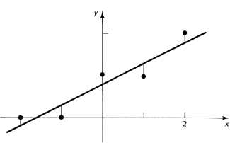
From the data (–2, 0), (–1, 0), (0, 1), (1, 1), and (2, 2), find the area under the curve from –2 to 2 using a least squares approximating straight line.
To find the line, we first make the table:
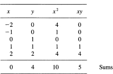
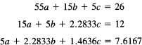
The normal equations for the straight line
y = a + bx
are
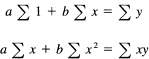
which are
![]()
From this we get a = 4/5, b = 1/2. The line looks about right, (see Figure 25.5-1), so we go ahead. Next, the integral
![]()
and we did not need the coefficient b, nor part of the table we computed. It pays to look ahead before you plunge into the routine details.
Example 25.5-2
Fit the given data (1, 5), (2, 3), (3, 2), (4, 1), and (5, 1) by the curve
![]()
Figure 25.5-1 Least squares line
and then estimate the derivative at x = 3, the midpoint.
This time (having learned from the previous example) we set up the normal equations first. We need to recall from Section 16.8 that we first write the least squares condition
![]()
to differentiate with respect to each parameter, and rearrange. We get for the normal equations
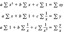
We now make the appropriate table:
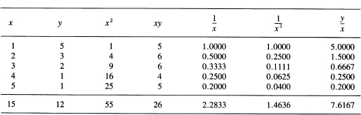
The normal equations are, therefore,
Before solving, let us ask what coefficients are needed? We have
![]()
Hence
![]()
We therefore eliminate b in the first stage of the solution. We get from the first two equations, and the second two equations,
![]()
From these c = 0.4096 and a = –0.9242. The derivative is, therefore,
y´(3) = –0.9697
It is worth finding b = 4.9855 to plot the data and curve to check the reasonableness of the derivative estimate (see Figure 25.5-2).
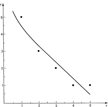
Figure 25.5-2 Least squares fit
1. Generalize Example 25.5-1 to 2N + 1 equally spaced points.
2. Find the integral under the curve in Example 25.5-2 [1, 5].
3. Given the data (0, 1), (1, 3), (2, 2), (3, 4), and (4, 4), find the integral under the least squares straight line from 0 to 4.
4. Using the data of Exercise 3, fit a quadratic and estimate the derivative at the origin.
25.6 ON FINDING FORMULAS
Which formula to use? That is a typical question in numerical methods when you stop and think about what you are doing. The direct method allows you to derive many different formulas to do the same job; for example, a low-order polynomial over a short interval or a higher-order polynomial over a longer interval (trapezoid over one interval and Simpson over a double interval are examples). The four questions raised in Section 25.2 must all be answered either consciously by choice or implicitly by picking a formula without thinking. We are better prepared to discuss the four choices now that a few numerical methods have been given.
1. What information to use? Generally, the closer the information is to where you are getting the answer, the better. It is almost true that a value of a derivative at a point is as good as another function value at some other place. As we noted, derivatives are apt to be much cheaper to compute than you at first think because of the large amount of machine time necessary to evaluate the special functions (including square root). As you can see from the direct method, each piece of information effectively determines one unknown parameter in the assumed form (Section 25.4).
2. What class of approximating functions to use? The great tendency of most people is to use polynomials without any careful thinking. But the direct method shows that the resulting formula is no more complex for other sets of linearly independent functions than it is for the polynomial formula. The derivation may be more difficult, but that is hardly a matter of great importance if the formula is to be used extensively. The right functions to use, generally, come from the nature of the problem and cannot be determined abstractly.
3. What criterion to use to select the specific function from the class? We have seen mainly exact matching and a little of least squares. There are other criteria such as minimax—the maximum error in the interval shall be minimum. This is an increasingly popular criterion as the faults of exact matching and least squares become better understood.
4. Where to apply the criterion? As you go on in numerical analysis, you will find that this question arises again and again, although it is often not explicitly stated but rather quietly assumed when you use the conventional methods. For example, when finding the zeros of a polynomial, is it the values of the zeros that you want to be accurate, the vanishing of the polynomial at the zeros to be accurate, or do you want to be able to reconstruct the polynomial from the computed zeros? Due to the inaccuracies of computing, these three things are not the same! Again, when finding a minimum, a broad curve leaves the position of the minimum ill determined, and a sharp minimum determines the location of the minimum quite well (see Figure 25.6-1). But when judged by the performance of the system, the broad minimum means that the performance is not degraded much for small changes, but the sharp minimum means that the system is sensitive to small changes. Which one do you want? Do not confuse, in numerical work with its inevitable small errors, accuracy in the solution values with accuracy in the property wanted.
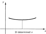
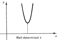
Figure 25.6-1
The author’s opinion is that with the direct method available we have reached the point in numerical methods where you should fit the formula to the problem, not the problem to the formula. In practice, the gathering of the data is usually so expensive in comparison to the data processing that care should be taken to get as much as you can from the given data.
1. Analyze the solution of the quadratic x2 + 80x + 1 = 0 for accuracy in the three senses given above, item 4.
2. Derive the equivalent of Simpson’s formula making it exact for 1, cos πx/2, and sin πx/2 for the double interval 0 ≤ x ≤ 1.
3. Derive the polynomial extension of Simpson’s formula when you use both the function and derivative values at each point. Discuss the corresponding composite formula.
25.7 INTEGRATION OF ORDINARY DIFFERENTIAL EQUATIONS
Once we can handle numerical integration, it is natural to turn to the numerical solution of ordinary differential equations. Frequently, the equations that arise cannot be solved in closed form, and numerical methods are necessary since the importance of the original problem is such that we must take some action. The numerical solution of ordinary differential equations is a vast subject, and we can give only the simpler methods and ideas involved.
The simplest method for integrating differential equations comes directly from the direction field (Section 23.2). You recall that after marking the slopes of the direction field you draw a smooth curve through them as best you can. This process can be mechanized easily. We will take a definite differential equation with a known solution (for check purposes) to illustrate the method before giving the general case.
Example 25.7-1
Given the differential equation
y' = 1 + y2 and y(0) = 0
find the solution. The slope at the point (0, 0) is, from the differential equation, 1. Suppose we go along this direction for a short distance, say ![]() x = 0.2. We will then be at the point
x = 0.2. We will then be at the point
(0.2, 0.2)
(see Figure 25.7-1). At this point the differential equation says that the slope is 1.04. We go along this direction for another step of ![]() x = 0.2 and get the point
x = 0.2 and get the point
(0.4, 0.408)
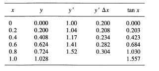
We repeat this process again and again. It is time to make a table of the numbers so we will not get lost, and so we can compare our solution with the known solution y = tan x.
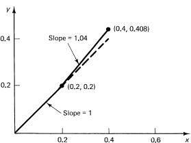
Figure 25.7-1 Numerical solution
TABLE 25.7-1
The answer is surprisingly good considering the step size. Obviously, decreasing the step size by a factor of 2 would decrease the error per step by about a factor of 4; but there would be twice as many steps, so the result would be about twice as accurate. Thus trying to get crude answers by this method is reasonable, but it is not a method for getting accurate answers without using a lot of computer time and incurring a lot of roundoff error in the process.
The fault of the method is immediately apparent: you are always using the slope that was and not the slope that is going to be. The crude formula we used cannot do what you did by eye in anticipating the new slope at the end of the interval as you drew the solution curve for the direction field solution. We need a better method that uses this simple observation.
Euler’s method does exactly this. It is a method that looks ahead, and then from the sample of the slope at the final end of the interval makes a new guess. In particular, with this new information Euler’s method tries again and does a better job at moving forward the step ![]() x by averaging the two slopes at the ends of the interval.
x by averaging the two slopes at the ends of the interval.
Let the equation and initial conditions be
y′ = f(x, y) and y0 = y(x0)
where we are starting at the point (xo, yo). We begin by assuming that the method is already going, and later we will discuss how to get started. We assume that you have the two most recent points on the curve (Figure 25.7-2). We will number the points by subscripts, which no longer are the arguments of the function. The formula
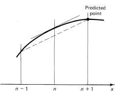
Figure 25.7-2 Euler´ predictor
![]()
reaches from the previous point yn-1, uses the current slope y′n, and predicts (hence the letter p) the next point (see Figure 25.7-2). At this point we make an estimate of the slope (from the derivative given by the differential equation):
![]()
Now using this slope together with the slope at xn, we can get an average slope for the interval [xn, xn+i], and hence the formula
![]()
gives a corrected value for the new point n + 1 (a more reliable point, probably, than the predicted value).
It remains to say how we can get started. One way is to realize that, when you differentiate the given differential equation, you get a formula for the second derivative at the initial point. Differentiation again gives the third derivative, and so on, so you can build up a Taylor series about the initial point and thus reach to the first point, which you need to get started.
Example 25.7-2
For the particular equation we are using
y' = 1 + y2
we have the successive derivatives
![]()
and at the point (0, 0) we have
![]()
Hence for the expansion about the origin we have
![]()
So at the point x = 0.2, we have, approximately,
![]()
as the first point from which Euler’s method takes off. We now make the beginning ofthe Table 25.7-2.
However, we note that the predicted value has an error of approximately ![]() x3ym(θ)/3 and the corrector has an error of about –(
x3ym(θ)/3 and the corrector has an error of about –(![]() x)3ym(θ)/12, so the difference is approximately
x)3ym(θ)/12, so the difference is approximately
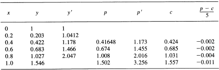
![]()
of which ![]() is due to the corrector (never mind that the θ values are not the same in the two formulas; we are only estimating an error). Thus we add this amount to the corrected value to get the final value
is due to the corrector (never mind that the θ values are not the same in the two formulas; we are only estimating an error). Thus we add this amount to the corrected value to get the final value
![]()
Correct value = 1.557; error = 0.011
This answer is significantly better than the answer from the crude method. This “mopping up” of the residual error in the corrector by adding (p – c)/5 is usually worth the effort as it is easy to do, and the computation of p – c gives you some control over the accuracy per step of the integration. When p – c gets too large, you need to halve the interval, using the formula
![]()
and, of course, using the differential equation to get the corresponding derivative. Alternatively, this can be done by simply restarting at the point where too much accuracy was being lost, lip – c gets too small, you can double the interval size and save computing effort. Thus, by changing step size as appropriate, you put the effort where it is needed and not where it is not.
In the days of computing by hand, the numerical solution of a differential equation was not undertaken lightly; but with hand calculators, especially programmable hand calculators, let alone small personal computers, the numerical solution of an ordinary differential equation is merely a matter of selecting a prewritten program, and programming the subroutines that describe the particular functions involved in the differential equation, along with the starting values and the desired accuracy.
We next turn briefly to the problem of integrating a system of first-order ordinary differential equations (Section 24.7). The method is exactly the same as for a single equation except that each equation has its values predicted in parallel, each derivative is then evaluated, each corrected value is computed (in parallel), and the final results for each variable are obtained before going on to the next interval. It is merely a great deal more work, since usually the right-hand-side functions for the derivatives involve a great deal more computing.
1. Integrate y´ = y2 + x2 from 0 to 1 using spacing h = 0.2, starting with y(0) = 1.
2. Integrate y´ = –y from 0 to 2 using h = 0.2 starting with y(0) = 1.
3. Integrate y´ = –xy starting with y(0) = 1, using spacing h = 0.1 and going to x = 2.
4. Derive the midpoint formula used in this section.
5. Integrate the system y´ = z, z´ = –y, y(0) = 0, y´(0) = 1, using h = 0.1 out to x = 3.2.
25.8 FOURIER SERIES AND POWER SERIES
A power series is a local approximation at a point; the partial sums fit the curve to higher- and higher-order derivatives. As a result, the quality of the approximation of the partial sum to the function is very good near the point about which the expansion is made, but gets poorer and poorer as you go away from the point. It is a local fit. On the other hand, the Fourier series is a least squares fit in the whole interval. No one point is made to be exceptionally good; the fit is designed to be uniformly good in the whole interval in the least squares sense. The fit is global (for the interval). Thus the two types of expansions do rather different things.
There is an interesting relationship between the two types of expansions, however. Suppose we have a power series partial sum
![]()
First we note that the way anyone who thinks about the matter evaluates a polynomial, as the above truncated power series is, by the chain method:
![]()
starting at the innermost multiplication and working outward.
Suppose, next, we make the change of variable
x = cos t
The expansion is now
![]()
This is a series in the powers of cos t; and for a Fourier series we want an expansion in multiples of the angle. There is a simple way of converting from the power series in cos t to the form of a Fourier series by using the identity
In words, the cosine of a given frequency when multiplied by cos t becomes one-half of the amount at the next higher frequency, plus one-half at the next lower frequency.
We use an inductive proof. The starting inner terms of the chain form are
an-1 + an cos t
This is a Fourier series! Multiply this by cos t and apply the above trigonometric identity (see Figure 25.8-1). The an-1 term becomes a cos term, but the coefficient of the cos term is divided by 2 and sent to both the one higher and the one lower frequency. We also add in the term an-2. We again have a Fourier series:
![]()
It is easy to see the general inductive step. Thus after the n – 1 stages in Figure 25.8-1, you have the Fourier series coefficients of the function fn(cos t).
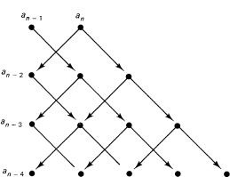
Figure 25.8-1 Conversion to Fourier series
There are several things to note. First, the process is clearly reversible. Second, in going from the power series form to the Fourier series form, the highest coefficient gets divided by 2n–1, and, in general, whatever the rate of decrease of the ak coefficients of the power series may be (as k increases), the coefficients of the Fourier series form decrease much more rapidly. But note that the sum of the coefficients is the same for both expansions; there is no loss in the sum of the coefficients.
If we now dropped the highest-frequency term of the Fourier series form, the change in the function would be not more than the size of the coefficient, since | cos t | ≤ 1 for all t. Indeed, we can drop as many terms from the Fourier series as we like as long as the sum of the absolute values of the coefficients does not exceed the error we are willing to commit.
This is the basis for a method called economization. We want to end up with an approximate least squares fit to a function whose power series we know. The plan is to take (1) more than enough terms of the power series, (2) convert to the Fourier series form, (3) drop the high-order terms, committing an additional error not more than the sum of the absolute values of the dropped terms, (4) convert back to the polynomial form, and the result is that we have a fit that is much like the Fourier series least squares approximation. The final transformation to the variable x merely stretches the x-axis and does not affect the quality of the fit very much (of course it affects the weights used in the fitting, but this is not large).
If we think in terms of the equal ripple property of the cosines, then what is going on is a bit clearer. We get the Fourier series form of the function and, since it is generally very rapidly converging, the error after dropping several terms tends to look like the last term dropped. The error committed is approximately equal ripple. Thus this equal ripple property is preserved when you go back from the t variable to the x variable. Economization tends to produce, from the power series approximation, an equal-ripple approximation good in the whole interval. The degree of the equal-ripple approximation can be significantly lower than the degree of the power series polynomial approximation of the same accuracy.
EXERCISES 25.8
1. Beginning with five terms of the exponential in the interval (0, 1), economize the series to three terms. Compare with three terms of the power series.
2. Find a series in x for the sine function in the interval (0, π/2) using a cubic final approximation.
3. Describe two ways of getting back from the Fourier series to the original power series.
25.9 SUMMARY
We have taken a very brief look at the vast and continually growing field of numerical analysis. Its main purpose is to find numerical solutions to problems that we cannot solve analytically, although at times we do evaluate functions that have been found in a suitable formula but that are too messy for us to grasp their meaning.
One of the main ideas of numerical analysis is analytic substitution; for the function we cannot handle, we substitute one we can and use some method of approximation so that the result we obtain is closely related to the answer we want. Polynomials are the classical functions to use, along with exact matching of the data, but more modem methods also use the Fourier series and other functions, as a basis; and we use exact matching of the data as well as least squares and other criteria for selecting the particular function from the class.
We have given you a powerful method for finding any of a very large class of formulas, polynomial or otherwise, and its great possibilities in adapting the formula to fit the problem should be understood.