The final reservoir type is the saturated oil reservoir and is distinguished by the presence of both liquid and gas in the reservoir. The material balance equations discussed in Chapter 6, for undersaturated oil reservoirs, apply to volumetric and water-drive reservoirs in which there are no initial gas caps. However, the equations apply to reservoirs in which an artificial gas-cap forms, owing either to gravitational segregation of the oil and free gas phases below the bubble point or to the injection of gas, usually in the higher structural portions of the reservoir. When there is an initial gas cap (i.e., the oil is initially saturated), there is negligible liquid expansion energy. However, the energy stored in the dissolved gas is supplemented by that in the cap, and it is not surprising that recoveries from gas-cap reservoirs are generally higher than from those without caps, other things remaining equal. This chapter will begin with a review of the factors that affect the overall recovery of saturated oil reservoirs and the application of the material balance used throughout the text. Drive indices, introduced in Chapter 3, are revisited, as they are most applicable to these types of reservoirs and quantitatively demonstrate the proportional effect of a given mechanism on the production. The Havlena-Odeh method will be applied to provide a tool for early prediction of reservoir behavior, followed by tools to understand and predict gas-liquid separation. The chapter will conclude with a discussion of volatile reservoirs and the concept of a maximum efficient rate (MER).
In gas-cap drives, as production proceeds and reservoir pressure declines, the expansion of the gas displaces oil downward toward the wells. This phenomenon is observed in the increase of the gas-oil ratios in successively lower wells. At the same time, by virtue of its expansion, the gas cap retards pressure decline and therefore the liberation of solution gas within the oil zone, thus improving recovery by reducing the producing gas-oil ratios of the wells. This mechanism is most effective in those reservoirs of marked structural relief, which introduces a vertical component of fluid flow, whereby gravitational segregation of the oil and free gas in the sand may occur.1 The recoveries from volumetric gas-cap reservoirs will typically be higher than the recoveries for undersaturated reservoirs and will be even higher for large gas caps, continuous uniform formations, and good gravitational segregation characteristics.
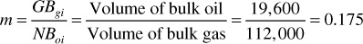
The size of the gas cap is usually expressed relative to the size of the oil zone by the ratio m, as defined in Chapter 3.
Continuous uniform formations reduce the channeling of the expanding gas cap ahead of the oil and the bypassing of oil in the less permeable portions.
These characteristics include primarily (1) pronounced structure, (2) low oil viscosity, (3) high permeability, and (4) low oil velocities.
Water drive and hydraulic control are terms used in designating a mechanism that involves the movement of water into the reservoir as gas and oil are produced. Water influx into a reservoir may be edgewater or bottomwater, the latter indicating that the oil is underlain by a water zone of sufficient thickness so that the water movement is essentially vertical. The most common source of water drive is a result of expansion of the water and the compressibility of the rock in the aquifer; however, it may result from artesian flow. The important characteristics of a water-drive recovery process are the following:
1. The volume of the reservoir is constantly reduced by the water influx. This influx is a source of energy in addition to the energy of liquid expansion above the bubble point and the energy stored in the solution gas and in the free, or cap, gas.
2. The bottom-hole pressure is related to the ratio of water influx to voidage. When the voidage only slightly exceeds the influx, there is only a slight pressure decline. When the voidage considerably exceeds the influx, the pressure decline is pronounced and approaches that for gas-cap or dissolved gas-drive reservoirs, as the case may be.
3. For edgewater drives, regional migration is pronounced in the direction of the higher structural areas.
4. As the water encroaches in both edgewater and bottomwater drives, there is an increasing volume of water produced, and eventually water is produced by all wells.
5. Under favorable conditions, the oil recoveries can be quite high.
The general Schilthuis material balance equation was developed in Chapter 3 and is as follows:
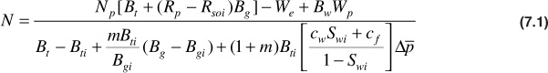
Equation (3.7) can be rearranged and solved for N, the initial oil in place:
If the expansion term due to the compressibilities of the formation and connate water can be neglected, as they usually are in a saturated reservoir, then Eq. (7.1) becomes
Example 7.1 shows the application of Eq. (7.2) to the calculation of initial oil in place for a water-drive reservoir with an initial gas cap. The calculations are done once by converting all barrel units to cubic feet units and then a second time by converting all cubic feet units to barrel units. It does not matter which set of units is used, only that each term in the equation is consistent. Problems sometimes arise because gas formation volume factors are reported either in ft3/SCF or in bbl/SCF. Typically, when applying the material balance equation for a liquid reservoir, gas formation volume factors are reported in bbl/SCF. Use care to ensure that the units are correct.
Example 7.1 Calculating the Stock-Tank Barrels of Oil Initially-in-Place in a Combination Drive Reservoir
Given
Volume of bulk oil zone = 112,000 ac-ft
Volume of bulk gas zone = 19,600 ac-ft
Initial reservoir pressure = 2710 psia
Initial formation volume factor = 1.340 bbl/STB
Initial gas volume factor = 0.006266 ft3/SCF
Initial dissolved GOR = 562 SCF/STB
Oil produced during the interval = 20 MM STB
Reservoir pressure at the end of the interval = 2000 psia
Average produced GOR = 700 SCF/STB
Two-phase formation volume factor at 2000 psia = 1.4954 bbl/STB
Volume of water encroached = 11.58 MM bbl
Volume of water produced = 1.05 MM STB
Formation volume factor of the water = 1.028 bbl/STB
Gas volume factor at 2000 psia = 0.008479 ft3/SCF
In the use of Eq. (7.2),
Bti = 1.3400 × 5.615 = 7.5241 ft3/STB
Bt = 1.4954 × 5.615 = 8.3967 ft3/STB
We = 11.58 × 5.615 = 65.02 MM ft3
Bw = 1.028 × 5.615 = 5.772 ft3/STB
BwWp = 1.028 × 5.615 × 1.05 = 6.06 MM res ft3
Assuming the same porosity and connate water for the oil and gas zones,
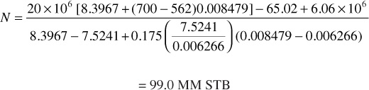
Substituting in Eq. (7.2) with all barrel units converted to cubic feet units,
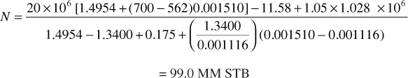
The calculation will be repeated using Eq. (7.2), with Bt in barrels per stock-tank barrel, Bg in barrels per standard cubic foot, and We and Wp in barrels.
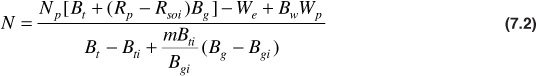
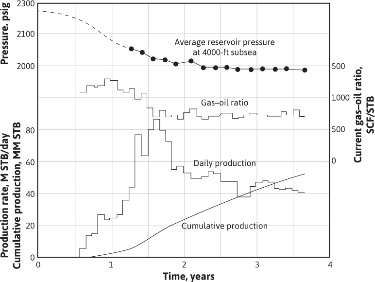
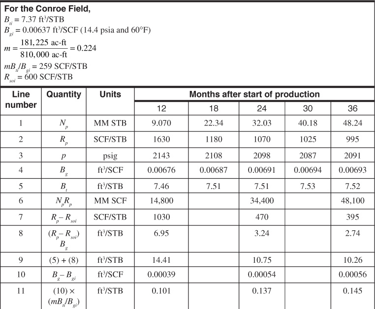
In Chapter 3, the concept of drive indices, first introduced to the reservoir engineering literature by Pirson, was developed.2 To illustrate the use of these drive indices, calculations are performed on the Conroe Field, Texas. Figure 7.1 shows the pressure and production history of the Conroe Field, and Fig. 7.2 gives the gas and two-phase oil formation volume factor for the reservoir fluids. Table 7.1 contains other reservoir and production data and summarizes the calculations in column form for three different periods.
Figure 7.1 Reservoir pressure and production data, the Conroe Field (after Schilthuis, trans. AlME).3
Figure 7.2 Pressure volume relations for the Conroe Field oil and original complement of dissolved gas (after Schilthuis, trans. AlME).3
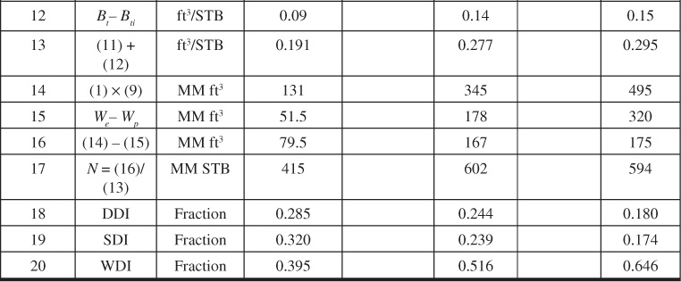
Table 7.1 Material Balance Calculation of Water Influx or Oil in Place for Oil Reservoirs below the Bubble-Point Pressure
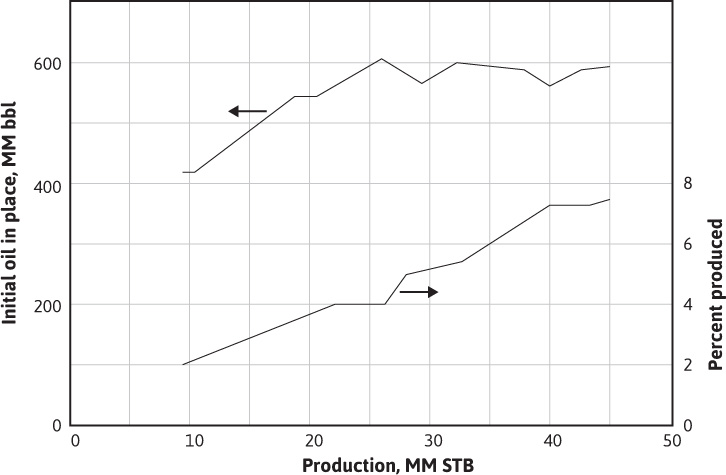
The use of such tabular forms is common in many calculations of reservoir engineering in the interest of standardizing and summarizing calculations that may not be reviewed or repeated for intervals of months or sometimes longer. The use of spreadsheets makes these calculations much easier and maintains the tabular form. They also enable an engineer to take over the work of a predecessor with a minimum of briefing and study. Tabular forms also have the advantage of providing at a glance the component parts of a calculation, many of which have significance themselves. The more important factors can be readily distinguished from the less important ones, and trends in some of the component parts often provide insight into the reservoir behavior. For example, the values of line 11 in Table 7.1 show the expansion of the gas cap of the Conroe Field as the pressure declines. Line 17 shows the values of the initial oil in place calculated at three production intervals. These values and others calculated elsewhere are plotted versus cumulative production in Fig. 7.3, which also includes the recovery at each period, expressed as the percentage of cumulative oil in the initial oil in place, as calculated at that period. The increasing values of the initial oil during the early life of the field may be explained by some of the limitations of the material balance equation discussed in Chapter 3, particularly the average reservoir pressure. Lower values of the average reservoir pressure in the more permeable and in the developed portion of the reservoir cause the calculated values of the initial oil to be low, through the effect on the oil and gas volume factors. The indications of Fig. 7.3 are that the reservoir contains approximately 600 MM STB of initial oil and that reliable values of the initial oil are not obtained until about 5% of the oil has been produced. This is not a universal figure but depends on a number of factors, particularly the amount of pressure decline. For the Conroe Field, the drive indices have been calculated at each of three periods, as given in lines 18, 19, and 20 of Table 7.1. For example, at the end of 12 months, the calculated initial oil in place is 415 MM STB, and the value of Np[Bt + (Rp – Rsoi)Bg] given in line 14 is 131 MM ft3. Then, from Eq. (3.11),
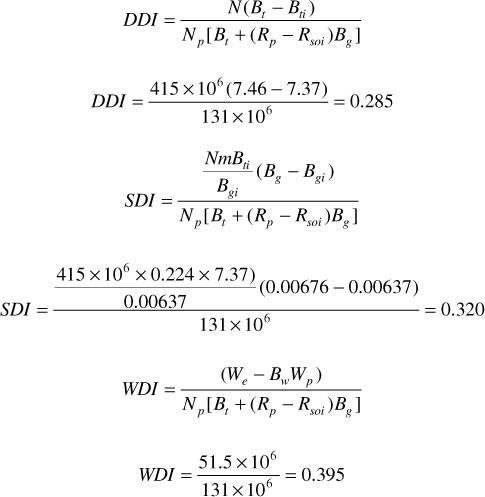
Figure 7.3 Active oil, the Conroe Field (after Schilthuis, trans. AlME).3
These figures indicate that, during the first 12 months, 39.5% of the production was by water drive, 32.0% by gas-cap expansion, and 28.5% by depletion drive. At the end of 36 months, as the pressure stabilized, the current mechanism was essentially 100% water drive and the cumulative mechanism increased to 64.6% water drive. If figures for recovery by each of the three mechanisms could be obtained, the overall recovery could be estimated using the drive indices. An increase in the depletion drive and gas-drive indices would be reflected by declining pressures and increasing gas-oil ratios and might indicate the need for water injection to supplement the natural water influx and to turn the recovery mechanism more toward water drive.
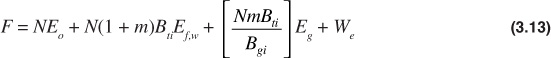
In Chapter 3, section 3.4, the method developed by Havlena-Odeh of applying the general material balance equation was presented.4,5 The Havlena-Odeh method is particularly advantageous for use early in the production life of a reservoir, as it adds constraints that aid in understanding how the reservoir is behaving. This understanding allows for more accurate prediction of production rates, pressure decline, and overall recovery. This method defines several new variables (see Chapter 3) and rewrites the material balance equation as Eq. (3.13):
This equation is then reduced for a particular application and arranged into a form of a straight line. When this is done, the slope and intercept often yield valuable assistance in determining such parameters as N and m. The usefulness of this approach is illustrated by applying the method to the data from the Conroe Field example discussed in the last section.
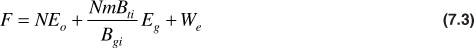
For the case of a saturated reservoir with an initial gas cap, such as the Conroe Field, and neglecting the compressibility term, Ef,w, Eq. (3.13) becomes
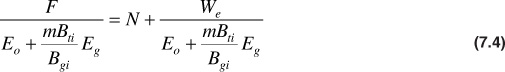
If N is factored out of the first two terms on the right-hand side and both sides of the equation are divided by the expression remaining after factoring, we get
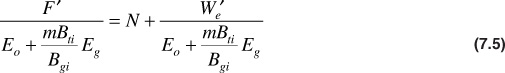
For the example of the Conroe Field in the previous section, the water production values were not known. For this reason, two dummy parameters are defined as F′ = F – WpBw and W′e = We – WpBw. Equation (7.4) then becomes
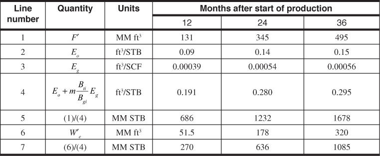
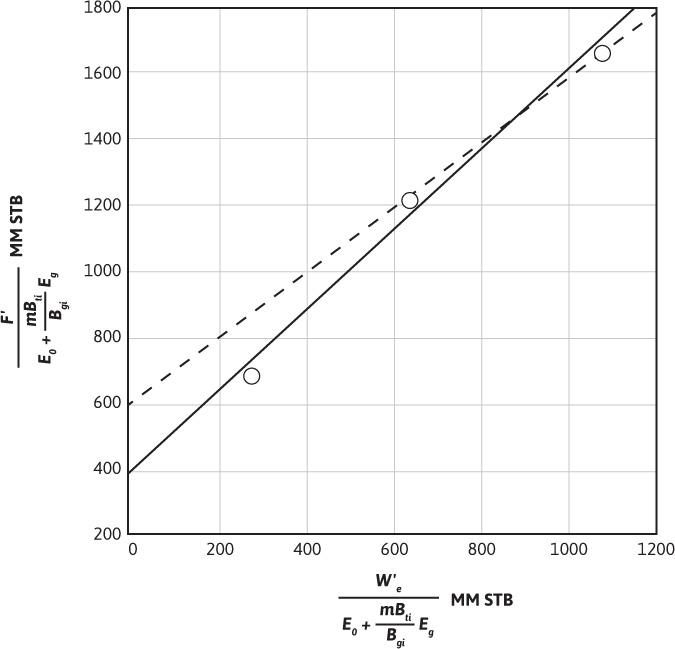
Equation (7.5) is now in the desired form. If a plot of F′/(Eo + mBtiEg/Bgi) as the ordinate and W′e/(Eo + mBtiEg/Bgi) as the abscissa is constructed, a straight line with slope equal to 1 and intercept equal to N is obtained. Table 7.2 contains the calculated values of the ordinate, line 5, and abscissa, line 7, using the Conroe Field data from Table 7.1. Figure 7.4 is a plot of these values.
Figure 7.4 Havlena-Odeh plot for the Conroe Field. Solid line represents line drawn through all data points. Dashed line represents line drawn through data points from the later production periods.
If a least squares regression analysis is done on all three data points calculated in Table 7.2, the result is the solid line shown in Fig. 7.4. The line has a slope of 1.21 and an intercept, N, of 396 MM STB. This slope is significantly larger than 1, which is what we should have obtained from the Havlena-Odeh method. If we now ignore the first data point, which represents the earliest production, and determine the slope and intercept of a line drawn through the remaining two points (the dashed line in Fig. 7.4), we get 1.00 for a slope and 600 MM STB for N, the intercept. This value of the slope meets the requirement for the Havlena-Odeh method for this case. We should now raise the question, can we justify ignoring the first point? If we realize that the production represents less than 5% of the initial oil in place and the fact that we have met the requirement for the slope of 1 for this case, then there is justification for not including the first point in our analysis. We conclude from our analysis that the initial oil in place is 600 MM STB for the Conroe Field.
The reader may take issue with the fact that an analysis was done on only two points. Clearly, it would have been better to use more data points, but none were available in this particular example. As more production data are collected, then the plot in Fig. 7.4 can be updated and the calculation for N reviewed. The important point to remember is that if the Havlena-Odeh method is used, the condition of the slope and/or intercept must be met for the particular case that is being worked. This imposes another restriction on the data and can be used to justify the exclusion of some data, as was done in the case of the Conroe Field example.
Fluid property data are extremely important pieces of information used in reservoir engineering calculations. It therefore becomes crucial to be knowledgeable about methods for obtaining these data. It is also important to relate those methods to what is occurring in the reservoir as gas evolves and then separates from the liquid phase. This section contains a discussion of two laboratory gas liberation processes as well as a discussion of the effect of surface separator operating pressures and temperatures.
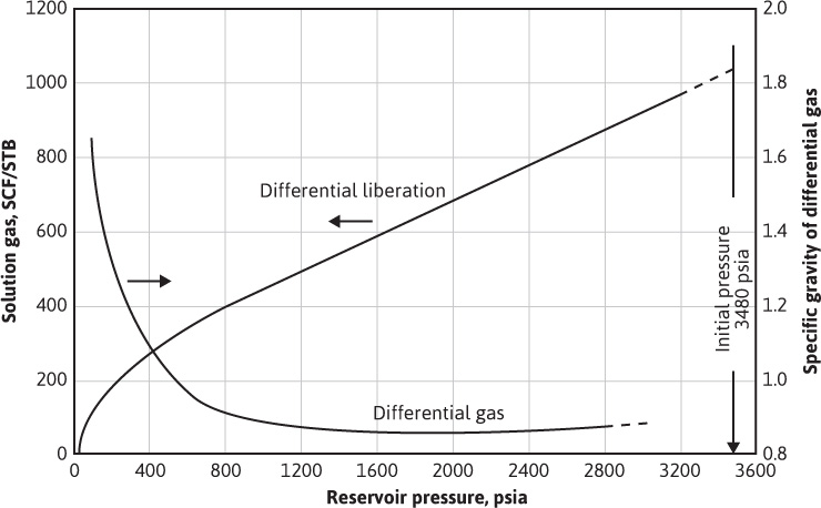
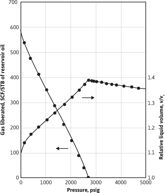
For heavy crudes whose dissolved gases are almost entirely methane and ethane, the manner of separation is relatively unimportant. For lighter crudes and heavier gases (i.e., for reservoir fluids with larger fractions of the intermediate hydrocarbons—mainly propane, butanes, and pentanes), the manner of separation raises some important questions. The nature of the difficulty lies mainly with these intermediate hydrocarbons that are, relatively speaking, intermediate between true gases and true liquids. They are therefore divided between the gas and liquid phases in proportions that are affected by the manner of separation. The situation may be explained with reference to two well-defined, isothermal, gas-liberation processes commonly used in laboratory pressure-volume-temperature (PVT) studies. In the flash liberation process, all the gas evolved during a reduction in pressure remains in contact and presumably in equilibrium with the liquid phase from which it is liberated. In the differential process, on the other hand, the gas evolved during a pressure reduction is removed from contact with the liquid phase as rapidly as it is liberated. Figure 7.5 shows the variation of solution gas with pressure for the differential process and the specific gravity of the gas that is being liberated at any pressure. Since the specific gravity of the gas is quite constant down to about 800 psia, it can be inferred that very close to the same quantity of gas would have been liberated by the flash process, down to 800 psia and at the same temperature. Below 800 psia, the vaporization of the intermediate hydrocarbons begins to be appreciable for the fluid of Fig. 7.5. In more volatile crudes, it begins at higher pressures and vice versa. The vaporization is indicated by the rise in the gas gravity and by the increasing rate of gas liberation, indicated by the steepening of the slope dRso/dp. If all the gas liberated down to, say, 400 psia remains in contact with the liquid phase, as in the flash process, more gas is liberated because the intermediate hydrocarbons in the liquid phase vaporize into the entire gas space in contact with the liquid until equilibrium is reached. Because gas is removed as rapidly as it is formed in the differential process, less vaporization of the intermediates occurs. The release of solution gas at lower pressures by the flash process, at the same temperature, is further accelerated because the loss of more of the intermediate hydrocarbons reduces the gas solubility. In some flash processes, the temperature is reduced at some pressure during the gas liberation process, whereas differential liberations are generally run at reservoir temperature. Because of the increased gas solubility and the lower volatility of the intermediates at lower temperatures, the quantity of gas released by the flash process is lower at the lower temperatures and is commonly less than the quantity released by the differential process at reservoir temperature.
Figure 7.5 Gas solubility and gas gravity by the differential liberation process on a subsurface sample from the Magnolia Field, Arkansas (after Carpenter, Schroeder, and Cook, US Bureau of Mines).6
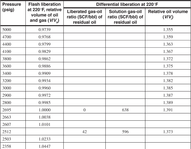
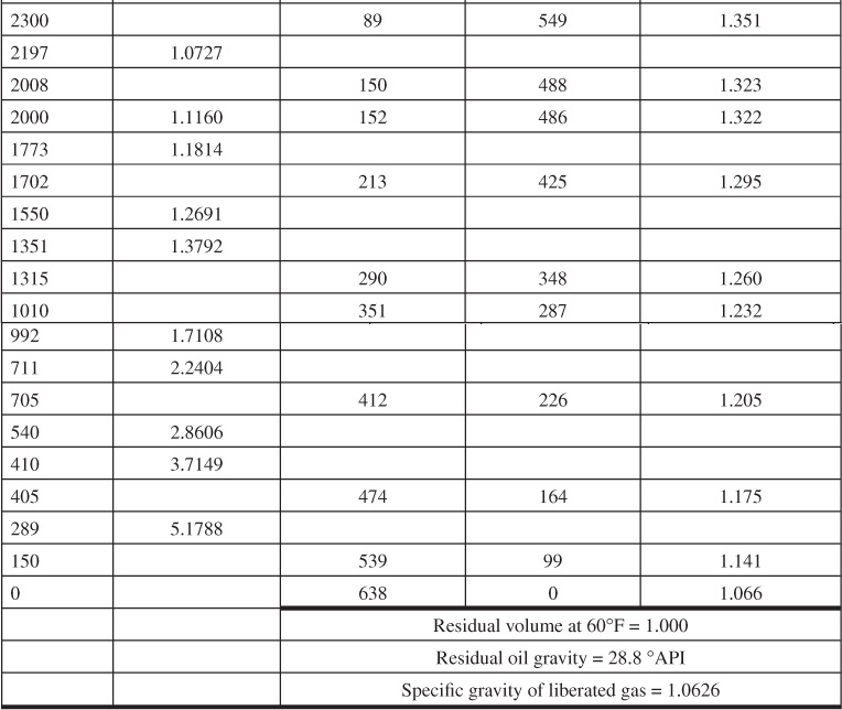
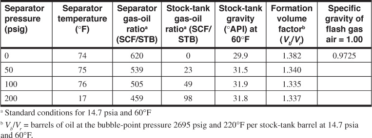
Table 7.3 gives the PVT data obtained from a laboratory study of a reservoir fluid sample at reservoir temperature of 220°F. The volumes given in the second column are the result of the flash gas-liberation process and are shown plotted in Fig. 7.6. Below the bubble-point pressure at 2695 psig, the volumes include the volume of the liberated gas and are therefore two-phase volume factors. Since the stock-tank oil remaining at atmospheric pressure depends on the pressure, temperature, and separation stages by which the gas is liberated at lower pressures, the volumes are reported relative to the volume at the bubble-point pressure, Vb. To relate the reservoir volumes to the stock-tank oil volumes, additional tests are performed on other samples using small-scale separators, which are operated in the range of pressures and temperatures used in the field separation of the gas and oil. Table 7.4 shows the results of four laboratory tests at separator pressures of 0, 50, 100, and 200 psig and separator temperatures from 74°F to 77°F. The temperatures are lower for the lower separator pressures because of the greater cooling effect of the gas expansion and the greater vaporization of the intermediate hydrocarbon components at the lower pressures. At 100 psig and 76°F, the tests indicate that 505 SCF are liberated at the separator and 49 SCF in the stock tank, or a total of 554 SCF/STB. Then the initial solution gas-oil ratio, Rsoi, is 554 SCF/STB. The tests also show that, under these separation conditions, 1.335 bbl of fluid at the bubble-point pressure yield 1.000 STB of oil. Hence, the formation volume factor at the bubble-point pressure is 1.335 bbl/STB, and the two-phase flash formation volume factor at 1773 psig is
Btf = 1.335 × 1.1814 = 1.577 bbl/STB
Figure 7.6 Flash liberation PVT data for a reservoir fluid at 220°F (after Kennerly, courtesy Core Laboratories, Inc.).
Table 7.4 Separator Tests of Reservoir Fluid Sample (after Kennerly, courtesy Core Laboratories, Inc.)
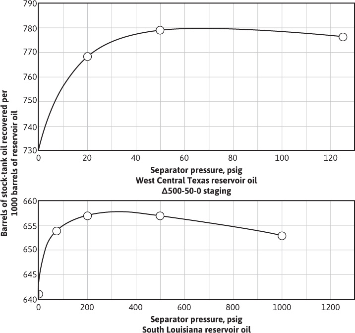
The data in Table 7.4 indicate that both oil gravity and recovery can be improved by using an optimum separator pressure of 100 psig and by reducing the loss of liquid components, particularly the intermediate hydrocarbons, to the separated gas. In reference to material balance calculations, they also indicate that the volume factors and solution gas-oil ratios depend on how the gas and oil are separated at the surface. When differing separation practices are used in the various wells owing to operator preference or to limitations of the flowing wellhead pressures, further complications are introduced. Figure 7.7 shows the variation in oil shrinkage with separator pressure for a west central Texas and a south Louisiana field. Each crude oil has an optimum separator pressure at which the shrinkage is a minimum and stock-tank oil gravity a maximum. For example, in the case of the west central Texas reservoir oil, there is an increased recovery of 7% when the operating separator pressure is increased from atmospheric pressure to 70 psig. The effect of using two stages of separation with the South Louisiana reservoir oil is shown by the triangle.
Figure 7.7 Variation in stock-tank recovery with separator pressure (after Kennerly, courtesy Core Laboratories, Inc.).
The effect of changes in separator pressures and temperatures on gas-oil ratios, oil gravities, and shrinkage in reservoir oil was determined for the Scurry Reef Field by Cook, Spencer, Bobrowski, and Chin.7,8 The data obtained from field and laboratory tests showed that the amount of gas liberated from the oil produced was affected materially by changes in both separator temperatures and pressures. For example, when the separator temperature was reduced to 62.5°F, the gas-oil ratio decreased from 1068 SCF/STB to 844 SCF/STB and the production increased from 125 STB/day to 135 STB/day. This was a decrease in gas-oil ratio of 21% and a production increase of 8%. Therefore, to yield the same volume of stock-tank oil, the production of 8% more reservoir fluid was needed when the separator was operating at the higher temperature.
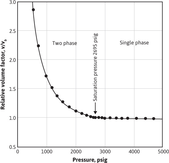
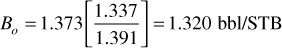
Table 7.3 also gives the solution gas and oil volume factors for the same reservoir fluid by differential liberation at 220°F, all the way down to atmospheric pressure, whereas the flash tests were stopped at 289 psig, owing to limitations of the volume of the PVT cell. Figure 7.8 shows a plot of the oil (liquid) volume factor and the liberated gas-oil ratios relative to a barrel of residual oil (i.e., the oil remaining at 1 atm and 60°F after a differential liberation down to 1 atm at 220°F). The volume change from 1.066 at 220°F to 1.000 at 60°F is a measure of the coefficient of thermal expansion of the residual oil. In some cases, a barrel of residual oil by the differential process is close to a stock-tank barrel by a particular flash process, and the two are taken as equivalent. In the present case, the volume factor at the bubble-point pressure is 1.335 bbl per stock-tank barrel by the flash process, using separation at 100 psig and 76°F versus 1.391 bbl per residual barrel by the differential process. The initial solution gas-oil ratios are 554 SCF/STB versus 638 SCF/residual barrel, respectively.
Figure 7.8 PVT data for the differential gas liberation of a reservoir fluid at 220°F (after Kennerly, courtesy Core Laboratories, Inc.).
In addition to the volumetric data of Table 7.3, PVT studies usually obtain values for (1) the specific volume of the bubble-point oil, (2) the thermal expansion of the saturated oil, and (3) the compressibility of the reservoir fluid at or above the bubble point. For the fluid of Table 7.3, the specific volume of the fluid at 220°F and 2695 psig is 0.02163 ft3/lb, and the thermal expansion is 1.07741 volumes at 220°F and 5000 psia per volume at 74°F and 5000 psia, or a coefficient of 0.00053 per °F. The compressibility of the undersaturated liquid has been discussed and calculated from the data of Table 7.3 in Chapter 2, section 2.6, as 10.27 × 10⁻⁶ psi–1 between 5000 psia and 4100 psia at 220°F.
The deviation factor of the gas released by the differential liberation process may be measured, or it may be estimated from the measured specific gravity. Alternatively, the gas composition may be calculated using a set of valid equilibrium constants and the composition of the reservoir fluid, and the gas deviation factor may be calculated from the gas composition.
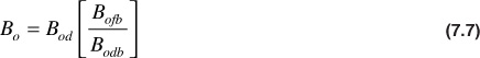
The data in Tables 7.3 and 7.4 can be combined to yield values for the oil formation volume factor and the solution gas-oil ratio. The formation volume factor is calculated from Eq. (7.6) or (7.7), depending on whether the pressure is above or below the bubble-point pressure: For p > bubble-point pressure,
For p < bubble-point pressure,
where
REV = Relative volume from the flash liberation test listed in Table 7.3 as V/Vb
Bofb = Formation volume factor from separator tests listed in Table 7.4 as Vb/Vr
Bod = Formation volume factor from differential liberation test listed in Table 7.3 as V/Vr
Bodb = Formation volume factor at the bubble point from differential liberation test
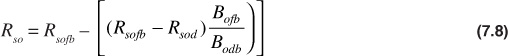
The solution gas-oil ratio can be calculated using Eq. (7.8),
where
Rsofb = Sum of separator gas and the stock-tank gas from separator tests listed in Table 7.4
Rsod = Solution gas-oil ratio from differential liberation test listed in Table 7.3
Rsodb = The value of Rsod at the bubble point
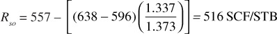
For example, at a pressure of 5000 psia and separator conditions of 200 psig and 77°F,
Bo = 0.9739 (1.337) = 1.302 bbl/STB
and
Rso = 459 + 98 = 557 SCF/STB
(Recall that Rso = Rsob for pressures above the bubble point.)
At a pressure of 2512 psig, which is below the bubble-point pressure, Bo and Rso become
and
If all gas in reservoirs was methane and all oil was decane and heavier, the PVT properties of the reservoir fluids would be quite simple because the quantities of oil and gas obtained from a mixture of the two would be almost independent of the temperatures, the pressures, and the type of the gas liberation process by which the two are separated. Low volatility crudes approach this behavior, which is approximately indicated by reservoir temperatures below 150°F, solution gas-oil ratios below 500 SCF/STB, and stock-tank gravities below 35 °API. Because the propane, butane, and pentane content of these fluids is low, the volatility is low.
For the conditions listed previously, but not too far above the approximate limits of low volatility fluids, satisfactory PVT data for material balance use are obtained by combining separator tests at appropriate temperatures and pressures with the flash and differential tests according to the procedure discussed in the previous section. Although this procedure is satisfactory for fluids of moderate volatility, it becomes less satisfactory as the volatility increases; more complicated, extensive, and precise laboratory tests are necessary to provide PVT data that are realistic in the application, particularly to reservoirs of the depletion type.
With present-day deeper drilling, many reservoirs of higher volatility are being discovered that include the gas-condensate reservoirs discussed in Chapter 5. The volatility is higher because of the higher reservoir temperatures at depth, approaching 500°F in some cases, and also because of the composition of the fluids, which are high in propane through decane. The volatile oil reservoir is recognized as a type intermediate in volatility between the moderately volatile reservoir and the gas-condensate reservoir. Jacoby and Berry have approximately defined the volatile type of reservoir as one containing relatively large proportions of ethane through decane at a reservoir temperature near or above 250°F, with a high formation volume factor and stock-tank oil gravity above 45 °API.9 The fluid of the Elk City Field, Oklahoma, is an example. The reservoir fluid at the initial pressure of 4364 psia and reservoir temperature of 180°F had a formation volume factor of 2.624 bbl/STB and a solution gas-oil ratio of 2821 SCF/STB, both relative to production through a single separator operating at 50 psig and 60°F. The stock-tank gravity was 51.4 °API for these separator conditions. Cook, Spencer, and Bobrowski described the Elk City Field and a technique for predicting recovery by depletion drive performance.10 Reudelhuber and Hinds and Jacoby and Berry also described somewhat similar laboratory techniques and prediction methods for the depletion drive performance of these volatile oil reservoirs.11,9 The methods are similar to those used for gas-condensate reservoirs discussed in Chapter 5.
A typical laboratory method of estimating the recovery from volatile reservoirs is as follows. Samples of primary separator gas and liquid are obtained and analyzed for composition. With these compositions and a knowledge of separator gas and oil flow rates, the reservoir fluid composition can be calculated. Also, by recombining the separator fluids in the appropriate ratio, a reservoir fluid sample can be obtained. This reservoir fluid sample is placed in a PVT cell and brought to reservoir temperature and pressure. At this point, several tests are conducted. A constant composition expansion is performed to determine relative volume data. These data are the flash liberation volume data listed in Table 7.3. On a separate reservoir sample, a constant volume expansion is performed while the volumes and compositions of the produced phases are monitored. The produced phases are passed through a separator system that simulates the surface facilities. By expanding the original reservoir fluid from the initial reservoir pressure down to an abandonment pressure, the actual production process from the reservoir is simulated. Using the data from the laboratory expansion, the field production can be estimated with a procedure similar to the one used in Example 5.3 to predict performance from a gas-condensate reservoir.
Many studies indicate that the recovery from true solution gas-drive reservoirs by primary depletion is essentially independent of both individual well rates and total or reservoir production rates. Keller, Tracy, and Roe showed that this is true even for reservoirs with severe permeability stratification where the strata are separated by impermeable barriers and are hydraulically connected only at the wells.12 The Gloyd-Mitchell zone of the Rodessa Field (see Chapter 6, section 6.5) is an example of a solution gas-drive reservoir that is essentially not rate sensitive (i.e., the recovery is unrelated to the rate at which the reservoir is produced). The recovery from very permeable, uniform reservoirs under very active water drives may also be essentially independent of the rates at which they are produced.
Many reservoirs are clearly rate sensitive and, for this reason, many governing bodies have imposed allowables that limit the production to a specified rate in order to ensure a maximum overall recovery of the well. These allowables are not typically reservoir specific and in conventional fields may be restrictive. Reservoir engineers can calculate a maximum efficient rate (MER) for a specific reservoir. Production at or below this rate will yield a maximum ultimate recovery, while production above this rate will result in a significant reduction in the practical ultimate oil recovery.13,14 Governing bodies have been known to adjust allowables for a reservoir when an MER has been proven.
Rate-sensitive reservoirs imply that there is some mechanism(s) at work in the reservoir that, in a practical period, can substantially improve the recovery of the oil in place. These mechanisms include (1) partial water drive, (2) gravitational segregation, and (3) those effective in reservoirs of heterogeneous permeability.
When initially undersaturated reservoirs are produced under partial water drive at voidage rates (gas, oil, and water) considerably in excess of the natural influx rate, they are produced essentially as solution gas-drive reservoirs modified by a small water influx. Assuming that recovery by water displacement is considerably larger than recovery by solution gas drive, there will be a considerable loss in recoverable oil by the high production rate, even when the oil zone is eventually entirely invaded by water. The loss is caused by the increase in the viscosity of the oil, the decrease in the volume factor of the oil at lower pressures, and the earlier abandonment of the wells that must be produced by artificial lift. Because of the higher oil viscosity at the lower pressure, producing water-oil ratios will be higher, and the economic limit of production rate will be reached at lower oil recoveries. Because of the lower oil volume factor at the lower pressure, at the same residual oil saturation in the invaded area, more stock-tank oil will be left at low pressure. There are, of course, additional benefits to be realized by producing at such a rate so as to maintain high reservoir pressure. If there is no appreciable gravitational segregation and the effects of reservoir heterogeneity are small, then the MER for a partial water-drive reservoir can be inferred from a study of the effect of the net reservoir voidage rate on reservoir pressure and the consequent effect of pressure on the gas saturation relative to the critical gas saturation (i.e., on gas-oil ratios). The MER may also be inferred from studies of the drive indices (Eq. [7.3]). The presence of a gas cap in a partial water-drive field introduces complications in determining the MER, which is affected by the relative size of the gas cap and the relative efficiencies of oil displacement by the expanding gas cap and by the encroaching water.
The Gloyd-Mitchell zone of the Rodessa Field was not rate sensitive because there was no water influx and because there was essentially no gravitational segregation of the free gas released from solution and the oil. If there had been substantial segregation, the well completion and well workover measures, which were taken in an effort to reduce gas-oil ratios, would have been effective, as they are in many solution gas-drive reservoirs. In some cases, a gas cap forms in the higher portions of the reservoir, and when high gas-oil ratio wells are penalized or shut in, there may be a substantial improvement in recovery, as indicated by Eq. (7.11), for a reduction in the value of the produced gas-oil ratio Rp. Under these conditions, the MER is that rate at which gravitational segregation is substantial for practical producing rates.
Gravitational segregation is also important in many gas-cap reservoirs. The effect of displacement rate on recovery by gas-cap expansion when there is substantial segregation of the oil and gas is discussed in Chapter 10. The studies presented on the Mile Six Pool show that, at the adopted displacement rate, the recovery will be approximately 52.4%. If the displacement rate is doubled, the recovery will be reduced to about 36.0%, and at very high rates, it will drop to 14.4% for negligible gravity segregation.
Gravitational segregation also occurs in the displacement of oil by water, and like the gas-oil segregation, it is also dependent on the time factor. Gravity segregation is generally of less relative importance in water drive than in gas-cap drive because of the much higher recoveries usually obtained by water drive. The MER for water-drive reservoirs is that rate above which there will be insufficient time for effective segregation and, therefore, a substantial loss of recoverable oil. The rate may be inferred from calculations similar to those used for gas displacement in Chapter 10 or from laboratory studies. It is interesting that, in the case of gravitational segregation, the reservoir pressure is not the index of the MER. In an active water-drive field, for example, there may be no appreciable difference in the reservoir pressure decline for a severalfold change in the production rate, and yet recovery at the lower rate may be substantially higher if gravity segregation is effective at the lower rate but not at the higher.
As water invades a reservoir of heterogeneous permeability, the displacement is more rapid in the more permeable portions, and considerable quantities of oil may be bypassed if the displacement rate is too high. At lower rates, there is time for water to enter the less permeable portions of the rock and recover a larger portion of the oil. As the water level rises, water is sometimes imbibed or drawn into the less permeable portions by capillary action, and this may also help recover oil from the less permeable areas. Because water imbibitions and the consequent capillary expulsion of oil are far from instantaneous, if appreciable additional oil can be recovered by this mechanism, the displacement rate should be lowered if possible. Although the MER under these circumstances is more difficult to establish, it may be inferred from the degree of the reservoir heterogeneity and the capillary pressure characteristics of the reservoir rocks.
In the present discussion of MER, it is realized that the recovery of oil is also affected by the reservoir mechanisms, fluid injection, gas-oil and water-oil ratio control, and other factors and that it is difficult to speak of rate-sensitive mechanisms entirely independently of these other factors, which in many cases are far more important.
7.1 Calculate the values for the second and fourth periods through the fourteenth step of Table 7.1 for the Conroe Field.
7.2 Calculate the drive indices at the Conroe Field for the second and fourth periods.
7.3 If the recovery by water drive at the Conroe Field is 70%, by segregation drive 50%, and by depletion drive 25%, using the drive indices for the fifth period, calculate the ultimate oil recovery expected at the Conroe Field.
7.4 Explain why the first material balance calculation at the Conroe Field gives a low value for the initial oil in place.
7.5 (a) Calculate the single-phase formation volume factor on a stock-tank basis, from the PVT data given in Tables 7.3 and 7.4 at a reservoir pressure of 1702 psig, for separator conditions of 100 psig and 76°F.
(b) Calculate the solution GOR at 1702 psig on a stock-tank basis for the same separator conditions.
(c) Calculate the two-phase formation volume factor by flash separation at 1550 psig for separator conditions of 100 psig and 76°F.
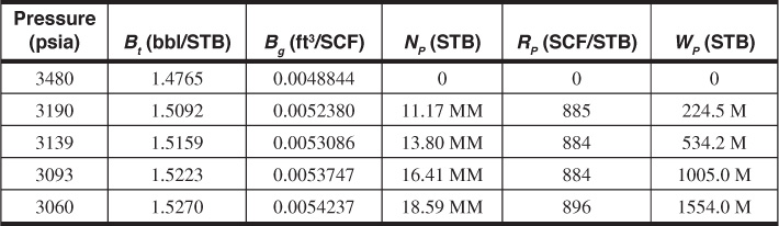
7.6 From the core data that follow, calculate the initial volume of oil and free gas in place by the volumetric method. Then, using the material balance equation, calculate the cubic feet of water that have encroached into the reservoir at the end of the four periods for which production data are given.
Average porosity = 16.8%
Connate water saturation = 27%
Productive oil zone volume = 346,000 ac-ft
Productive gas zone volume = 73,700 ac-ft
Bw= 1.025 bbl/STB
Reservoir temperature = 207°F
Initial reservoir pressure = 3480 psia
7.7 The following PVT data are for the Aneth Field in Utah:
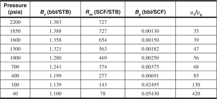
The initial reservoir temperature was 133°F. The initial pressure was 2200 psia, and the bubble-point pressure was 1850 psia. There was no active water drive. From 1850 psia to 1300 psia, a total of 720 MM STB of oil and 590.6 MMM SCF of gas was produced.
(a) How many reservoir barrels of oil were in place at 1850 psia?
(b) The average porosity was 10%, and connate water saturation was 28%. The field covered 50,000 acres. What is the average formation thickness in feet?
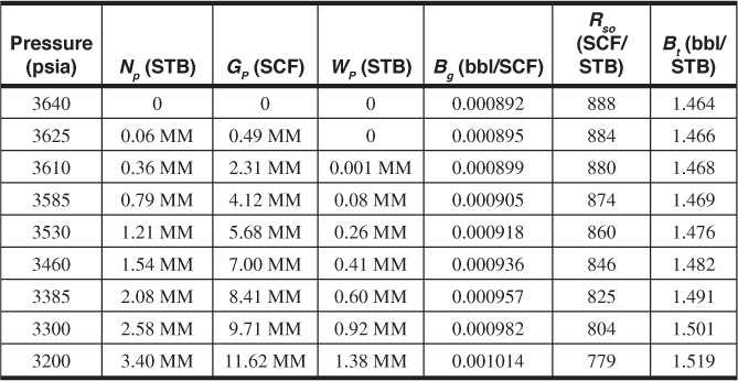
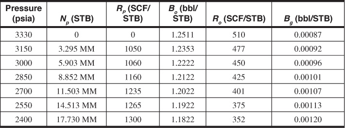
7.8 You have been asked to review the performance of a combination solution gas, gas-cap drive reservoir. Well test and log information show that the reservoir initially had a gas cap half the size of the initial oil volume. Initial reservoir pressure and solution gas-oil ratio were 2500 psia and 721 SCF/STB, respectively. Using the volumetric approach, initial oil in place was found to be 56 MM STB. As you proceed with the analysis, you discover that your boss has not given you all the data you need to make the analysis. The missing information is that, at some point in the life of the project, a pressure maintenance program was initiated using gas injection. The time of the gas injection and the total amount of gas injected are not known. There was no active water drive or water production. PVT and production data are in the following table:
(a) At what point (i.e., pressure) did the pressure maintenance program begin?
(b) How much gas in SCF had been injected when the reservoir pressure was 500 psia? Assume that the reservoir gas and the injected gas have the same compressibility factor.
7.9 An oil reservoir initially contains 4 MM STB of oil at its bubble-point pressure of 3150 psia, with 600 SCF/STB of gas in solution. When the average reservoir pressure has dropped to 2900 psia, the gas in solution is 550 SCF/STB. Boi was 1.34 bbl/STB and Bo at a pressure of 2900 psia is 1.32 bbl/STB.
Some additional data are as follows:
Rp = 600 SCF/STB at 2900 psia
Swi = 0.25
Bg = 0.0011 bbl/SCF at 2900 psia
This is a volumetric reservoir.
There is no original gas cap.
(a) How many STB of oil will be produced when the pressure has decreased to 2900 psia?
(b) Calculate the free gas saturation that exists at 2900 psia.
7.10 Given the following data from laboratory core tests, production data, and logging information, calculate the water influx and the drive indices at 2000 psia:
Well spacing = 320 ac
Net pay thickness = 50 ft with the gas/oil contact 10 ft from the top
Porosity = 0.17
Overall initial water saturation in the net pay = 0.26
Overall initial gas saturation in the net pay = 0.15
Bubble-point pressure = 3600 psia
Initial reservoir pressure = 3000 psia
Reservoir temperature = 120°F
Boi = 1.26 bbl/STB
Bo = 1.37 bbl/STB at the bubble-point pressure
Bo = 1.19 bbl/STB at 2000 psia
Np = 2.0 MM STB at 2000 psia
Gp = 2.4 MMM SCF at 2000 psia
Gas compressibility factor, z = 1.0 – 0.0001p
Solution gas-oil ratio, Rso = 0.2p
7.11 From the following information, determine
(a) Cumulative water influx at pressures 3625, 3530, and 3200 psia
(b) Water-drive index for the pressures in (a)
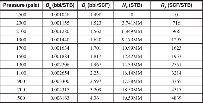
7.12 The cumulative oil production, Np, and cumulative gas oil ratio, Rp, as functions of the average reservoir pressure over the first 10 years of production for a gas-cap reservoir, are as follows. Use the Havlena-Odeh approach to solve for the initial oil and gas (both free and solution) in place.
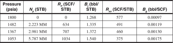
7.13 Using the following data, determine the original oil in place by the Havlena-Odeh method. Assume there is no water influx and no initial gas cap. The bubble-point pressure is 1800 psia.
1. Petroleum Reservoir Efficiency and Well Spacing, Standard Oil Development Company, 1934, 24.
2. Sylvain J. Pirson, Elements of Oil Reservoir Engineering, 2nd ed., McGraw-Hill, 1958, 635–93.
3. Ralph J. Schilthuis, “Active Oil and Reservoir Energy,” Trans. AlME (1936), 118, 33.
4. D. Havlena and A. S. Odeh, “The Material Balance as an Equation of a Straight Line,” Jour. of Petroleum Technology (Aug. 1963), 896–900.
5. D. Havlena and A. S. Odeh, “The Material Balance as an Equation of a Straight Line: Part II—Field Cases,” Jour. of Petroleum Technology (July 1964), 815–22.
6. Charles B. Carpenter, H. J. Shroeder, and Alton B. Cook, “Magnolia Oil Field, Columbia County, Arkansas,” US Bureau of Mines, R.I. 3720, 1943, 46, 47, 82.
7. Alton B. Cook, G. B. Spencer, F. P. Bobrowski, and Tim Chin, “Changes in Gas-Oil Ratios with Variations in Separator Pressures and Temperatures,” Petroleum Engineer (Mar. 1954), 26, B77–B82.
8. Alton B. Cook, G. B. Spencer, F. P. Bobrowski, and Tim Chin, “A New Method of Determining Variations in Physical Properties in a Reservoir, with Application to the Scurry Reef Field, Scurry County, Texas,” US Bureau of Mines, R.I. 5106, Feb. 1955, 10–11.
9. R. H. Jacoby and V. J. Berry Jr., “A Method for Predicting Depletion Performance of a Reservoir Producing Volatile Crude Oil,” Trans. AlME (1957), 201, 27.
10. Alton B. Cook, G. B. Spencer, and F. P. Bobrowski, “Special Considerations in Predicting Reservoir Performance of Highly Volatile Type Oil Reservoirs,” Trans. AlME (1951), 192, 37–46.
11. F. O. Reudelhuber and Richard F. Hinds, “A Compositional Material Balance Method for Prediction of Recovery from Volatile Oil Depletion Drive Reservoirs,” Trans. AlME (1957), 201, 19–26.
12. W. O. Keller, G. W. Tracy, and R. P. Roe, “Effects of Permeability on Recovery Efficiency by Gas Displacement,” Drilling and Production Practice, API (1949), 218.
13. Edgar Kraus, “MER—A History,” Drilling and Production Practice, API (1947), 108–10.
14. Stewart E. Buckley, Petroleum Conservation, American Institute of Mining and Metallurgical Engineers, 1951, 151–63.