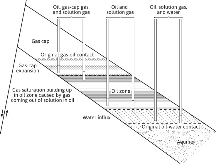
Figure 3.1 Cross section of a combination drive reservoir (after Woody and Moscrip, trans. AlME).5
Fluid does not leave a void space behind, as it is produced from a hydrocarbon reservoir. As the pressure in the reservoir drops during the production of fluids, the remaining fluids and/or reservoir rock expand or nearby water encroaches to fill the space created by any produced fluids. The volume of oil produced on the surface aids the reservoir engineer in determining the amount of the expansion or encroachment that occurs in the reservoir. Material balance is a method that can be used to account for the movement of reservoir fluids within the reservoir or to the surface where they are produced. The material balance accounts for the fluid produced from the reservoir through expansion of existing fluid, expansion of the rock, or the migration of water into the reservoir. A general material balance equation that can be applied to all reservoir types is developed in this chapter. The material balance equation includes factors that compare the various compressibilities of fluids, consider the gas saturated in the liquid phase, and include the water that may enter into the hydrocarbon reservoir from a connected aquifer. From this general equation, each of the individual equations for the reservoir types defined in Chapter 1 and discussed in subsequent chapters can easily be derived by considering the impact of the various terms of the material balance equation.
The general material balance equation was first developed by Schilthuis in 1936.1 Since that time, the use of computers and sophisticated multidimensional mathematical models have replaced the zero-dimensional Schilthuis equation in many applications.2 However, the Schilthuis equation, if fully understood, can provide great insight for the practicing reservoir engineer. Following the derivation of the general material balance equation, a method of using the equation discussed in the literature by Havlena and Odeh is presented.3,4
When an oil and gas reservoir is tapped with wells, oil and gas, and frequently some water, are produced, thereby reducing the reservoir pressure and causing the remaining oil and gas to expand to fill the space vacated by the fluids removed. When the oil- and gas-bearing strata are hydraulically connected with water-bearing strata (aquifers) with bulk volume much greater than that of the hydrocarbon zone, water encroaches into the reservoir as the pressure drops owing to production, as illustrated in Fig. 3.1. This water encroachment decreases the extent to which the remaining oil and gas expand and accordingly retards the decline in reservoir pressure. Inasmuch as the temperature in oil and gas reservoirs remains substantially constant during the course of production, the degree to which the remaining oil and gas expand depends on the pressure and the composition of the oil and gas. By taking bottom-hole samples of the reservoir fluids under pressure and measuring their relative volumes in the laboratory at reservoir temperature and under various pressures, it is possible to predict how these fluids behave in the reservoir as reservoir pressure declines.
Figure 3.1 Cross section of a combination drive reservoir (after Woody and Moscrip, trans. AlME).5
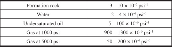
In Chapter 6, it is shown that, although the connate water and formation compressibilities are quite small, they are, relative to the compressibility of reservoir fluids above their bubble points, significant, and they account for an appreciable fraction of the production above the bubble point. Table 3.1 gives a range of values for formation and fluid compressibilities from which it may be concluded that water and formation compressibilities are less significant in gas and gas cap reservoirs and in undersaturated reservoirs below the bubble point where there is appreciable gas saturation. Because of this and the complications they would introduce in already fairly complex equations, water and formation compressibilities are generally neglected, except in undersaturated reservoirs producing above the bubble point. A term accounting for the change in water and formation volumes owing to their compressibilities is included in the material balance derivation, and the engineer can choose to eliminate this for particular applications. The gas in solution in the formation water is neglected, and in many instances, the volume of the produced water is not known with sufficient accuracy to justify the use of a formation volume factor with the produced water.
The general material balance equation is simply a volumetric balance, which states that since the volume of a reservoir (as defined by its initial limits) is a constant, the algebraic sum of the volume changes of the oil, free gas, water, and rock volumes in the reservoir must be zero. For example, if both the oil and gas reservoir volumes decrease, the sum of these two decreases must be balanced by changes of equal magnitude in the water and rock volumes. If the assumption is made that complete equilibrium is attained at all times in the reservoir between the oil and its solution gas, it is possible to write a generalized material balance expression relating the quantities of oil, gas, and water produced; the average reservoir pressure; the quantity of water that may have encroached from the aquifer; and finally the initial oil and gas content of the reservoir. In making these calculations, the following production, reservoir, and laboratory data are involved:
1. The initial reservoir pressure and the average reservoir pressure at successive intervals after the start of production.
2. The stock-tank barrels of oil produced, measured at 1 atm and 60°F, at any time or during any production interval.
3. The total standard cubic feet of gas produced. When gas is injected into the reservoir, this will be the difference between the total gas produced and that returned to the reservoir.
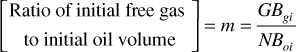
4. The ratio of the initial gas cap volume and the initial oil volume, m:
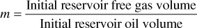
If the value of m can be determined with reasonable precision, there is only one unknown (N) in the material balance on volumetric gas cap reservoirs and two (N and We) in water-drive reservoirs. The value of m is determined from log and core data and from well completion data, which frequently helps to locate the gas-oil and water-oil contacts. The ratio m is known in many instances much more accurately than the absolute values of the gas cap and oil zone volumes. For example, when the rock in the gas cap and that in the oil zone appear to be essentially the same, it may be taken as the ratio of the net or even the gross volumes (without knowing the average connate water or average porosity).
5. The gas and oil formation volume factors and the solution gas-oil ratios. These are obtained as functions of pressure by laboratory measurements on bottom-hole samples by the differential and flash liberation methods.
6. The quantity of water that has been produced.
7. The quantity of water that has been encroached into the reservoir from the aquifer.
For simplicity, the derivation is divided into the changes in the oil, gas, water, and rock volumes that occur between the start of production and any time t. The change in the rock volume is expressed as a change in the pore volume, which is simply the negative of the change in the rock volume. In the development of the general material balance equation, the following terms are used:
N
Initial reservoir oil, STB
Boi
Initial oil formation volume factor, bbl/STB
Np
Cumulative produced oil, STB
Bo
Oil formation volume factor, bbl/STB
G
Initial reservoir gas, SCF
Bgi
Initial gas formation volume factor, bbl/SCF
Gf
Amount of free gas in the reservoir, SCF
Rsoi
Initial solution gas-oil ratio, SCF/STB
Rp
Cumulative produced gas-oil ratio, SCF/STB
Rso
Solution gas-oil ratio, SCF/STB
Bg
Gas formation volume factor, bbl/SCF
W
Initial reservoir water, bbl
Wp
Cumulative produced water, STB
Bw
Water formation volume factor, bbl/STB
We
Water influx into reservoir, bbl
c
Total isothermal compressibility, psi–1
Δ
Change in average reservoir pressure, psia
Swi
Initial water saturation
Vf
Initial pore volume, bbl
cf
Formation isothermal compressibility, psi–1
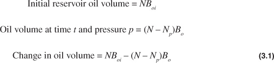
The following expression determines the change in the oil volume:
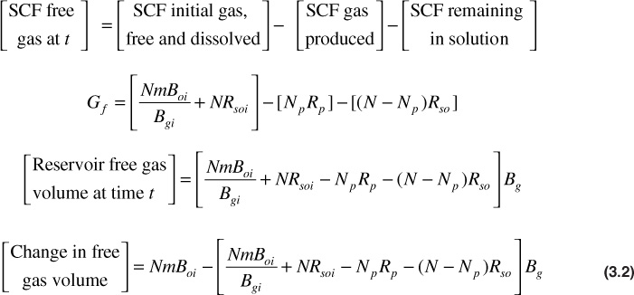
The following expression determines the change in free gas volume:
When initial free gas volume = GBgi = NmBoi,
The following expression determines the change in the water volume:
Initial reservoir water volume = W
Cumulative water produced at t = Wp
Reservoir volume of cumulative produced water = Bw Wp
Volume of water encroached at t = We
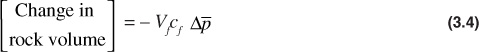
The following expression determines the change in the void space volume:
Initial void space volume = Vf
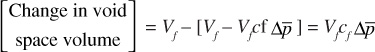
Or, because the change in void space volume is the negative of the change in rock volume,
Combining the changes in water and rock volumes into a single term yields the following:

Recognizing that W = VfSwi and 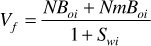 and substituting, the following is obtained:
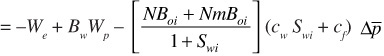
or
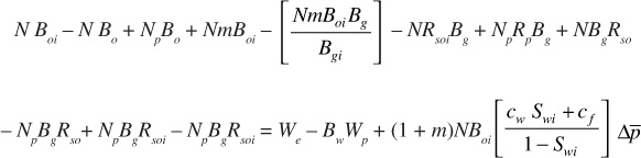
Equating the changes in the oil and free gas volumes to the negative of the changes in the water and rock volumes and expanding all terms produces
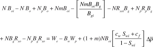
Adding and subtracting the term NpBgRsoi produces
Then, grouping terms produces
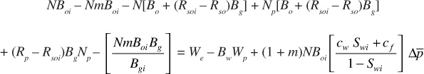
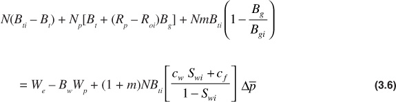
Writing Boi = Bti and [Bo + (Rsoi – Rso)Bg] = Bt, where Bt is the two-phase formation volume factor, as defined by Eq. (2.29), produces
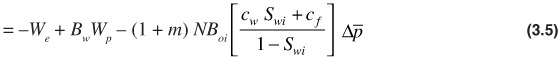
This is the general volumetric material balance equation. It can be rearranged into the following form, which is useful for discussion purposes:
Each term on the left-hand side of Eq. (3.7) accounts for a method of fluid production, and each term on the right-hand side represents an amount of hydrocarbon or water production. For illustration purposes, Eq. (3.7) can be written as follows, with each mathematical term replaced by a pseudoterm:
The left-hand side accounts for all the methods of expansion or influx in the reservoir that would drive the production of oil, gas, and water, the terms on the right-hand side. Oil expansion is derived from the product of the initial oil in place and the change in the two-phase oil formation volume factor. Gas expansion is similar; however, additional terms are needed to convert the initial oil in place to initial gas in place—both free gas and dissolved gas. The third term can be broken down into three pieces. It is the product of the initial oil and gas in place, the expansion of the connate water and the formation rock, and the change in the volumetric average reservoir pressure. These three pieces account for the expansion of the connate water and the formation rock in the reservoir.
On the right-hand side, the oil and gas produced is determined by considering the volume of the produced oil if it were in the reservoir. The produced oil is multiplied by the sum of the two-phase oil formation volume factor and the volume factor of gas liberated as the pressure has declined. The produced water is simply the product of the produced water and its volume factor.
Equation (3.7) can be arranged to apply to any of the different reservoir types discussed in Chapter 1. Without eliminating any terms, Eq. (3.7) is used for the case of a saturated oil reservoir with an associated gas cap. These reservoirs are discussed in Chapter 7. When there is no original free gas, such as in an undersaturated oil reservoir (discussed in Chapter 6), m = 0, and Eq. (3.7) reduces to
For gas reservoirs, Eq. (3.7) can be modified by recognizing that NPRP = Gp and NmBti = GBgi and substituting these terms into Eq. (3.7):
When working with gas reservoirs, there is no initial oil amount; therefore, N and Np equal zero. The general material balance equation for a gas reservoir can then be obtained:
This equation is discussed in conjunction with gas and gas-condensate reservoirs in Chapters 4 and 5.
In the study of reservoirs that are produced simultaneously by the three major mechanisms of depletion drive, gas cap drive, and water drive, it is of practical interest to determine the relative magnitude of each of these mechanisms that contribute to the production. Pirson rearranged the material balance Eq. (3.7) as follows to obtain three fractions, whose sum is one, which he called the depletion drive index (DDI), the segregation (gas cap) drive index (SDI), and the water-drive index (WDI).6
When all three drive mechanisms are contributing to the production of oil and gas from the reservoir, the compressibility term in Eq. (3.7) is negligible and can be ignored. Moving the water production term to the left-hand side of the equation, the following is obtained:

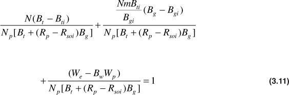
Dividing through by the term on the right-hand side of the equation produces
The numerators of the three fractions that appear on the left-hand side of Eq. (3.11) are the expansion of the initial oil zone, the expansion of the initial gas zone, and the net water influx, respectively. The common denominator is the reservoir volume of the cumulative gas and oil production expressed at the lower pressure, which evidently equals the sum of the gas and oil zone expansions plus the net water influx. Then, using Pirson’s abbreviations,
DDI + SDI + WDI = 1
calculations are performed in Chapter 7 to illustrate how these drive indices can be used.
The material balance equation derived in the previous section has been in general use for many years, mainly for the following:
1. Determining the initial hydrocarbon in place
2. Calculating water influx
3. Predicting reservoir pressures
Although in some cases it is possible to solve simultaneously to find the initial hydrocarbon and the water influx, generally one or the other must be known from data or methods that do not depend on the material balance calculations. One of the most important uses of the equations is predicting the effect of cumulative production and/or injection (gas or water) on reservoir pressure; therefore, it is very desirable to know in advance the initial oil and the ratio m from good core and log data. The presence of an aquifer is usually indicated by geologic evidence; however, the material balance may be used to detect the existence of a water drive by calculating the value of the initial hydrocarbon at successive production periods, assuming zero water influx. Unless other complicating factors are present, the constancy in the calculated value of N and/or G indicates a volumetric reservoir, and continually changing values of N and G indicate a water drive.
The precision of the calculated values depends on the accuracy of the data available to substitute in the equation and on the several assumptions that underlie the equations. One such assumption is the attainment of thermodynamic equilibrium in the reservoir, mainly between the oil and its solution gas. Wieland and Kennedy have found a tendency for the liquid phase to remain supersaturated with gas as the pressure declines.7 Saturation pressure discrepancies between fluid and core measurements and material balance evidence in the range of 19 psi for the East Texas Field and 25 psi for the Slaughter Field were observed. The effect of supersaturation causes reservoir pressure for a given volume of production to be lower than it otherwise would have been, had equilibrium been attained.
It is also implicitly assumed that the PVT data used in the material balance analyses are obtained using gas liberation processes that closely duplicate the gas liberation processes in the reservoir, in the well, and in separators on the surface. This matter is discussed in detail in Chapter 7, and it is only stated here that PVT data based on gas liberation processes that vary widely from the actual reservoir development can cause considerable error in the material balance results and implications.
Another source of error is introduced in the determination of average reservoir pressure at the end of any production interval. Aside from instrument errors and those introduced by difficulties in obtaining true static or final buildup pressures (see Chapter 8), there is often the problem of correctly weighting or averaging the individual well pressures. For thicker formations with higher permeabilities and oils of lower viscosities, where final buildup pressures are readily and accurately obtained and when there are only small pressure differences across the reservoir, reliable values of average reservoir pressure are easily obtained. On the other hand, for thinner formations of lower permeability and oils of higher viscosity, difficulties are met in obtaining accurate final buildup pressures, and there are often large pressure variations throughout the reservoir. These are commonly averaged by preparing isobaric maps superimposed on isopach maps. This method usually provides reliable results unless the measured well pressures are erratic and therefore cannot be accurately contoured. These differences may be due to variations in formation thickness and permeability and in well production and producing rates. Also, difficulties are encountered when production from two or more vertically isolated zones or strata of different productivity are commingled. In this case, the pressures are generally higher in the strata of low productivity, and because the measured pressures are nearer to those in the zones of high productivity, the measured static pressures tend to be lower and the reservoir behaves as if it contained less oil. Schilthuis explained this phenomenon by referring to the oil in the more productive zones as active oil and by observing that the calculated active oil usually increases with time because the oil and gas in the zones of lower productivity slowly expand to help offset the pressure decline. Uncertainties associated with assessing production from commingled reservoir zones motivate regulatory restrictions for this reservoir management strategy. Fields that are not fully developed may also show similar apparent increase in active oil production because the apparent average pressure can be that of the developed portion only while the pressure is actually higher in the undeveloped portions.
The effect of pressure errors on calculated values of initial oil or water influx depends on the size of the errors in relation to the reservoir pressure decline. This is true because pressure enters the material balance equation mainly as differences (Bo – Boi), (Rsi – Rs), and (Bg – Bgi). Because water influx and gas cap expansion tend to offset pressure decline, the pressure errors are more serious than for the undersaturated depletion reservoirs. In the case of very active water drives and gas caps that are large compared with the associated oil zone, the material balance is useless to determine the initial oil in place because of the very small pressure decline. Hutchinson emphasized the importance of obtaining accurate values of static well pressures in his quantitative study of the effect of data errors on the values of initial gas or of initial oil in volumetric gas or undersaturated oil reservoirs, respectively.8
Uncertainties in the ratio of the initial free gas volume to the initial reservoir oil volume also affect the calculations. The error introduced in the calculated values of initial oil, water influx, or pressure increases with the size of this ratio because, as explained in the previous paragraph, larger gas caps reduce the effect of pressure decline. For quite large gas caps relative to the oil zone, the material balance approaches a gas balance modified slightly by production from the oil zone. The value of m is obtained from core and log data used to determine the net productive bulk gas and oil volumes and their average porosities and interstitial water. Because there is frequently oil saturation in the gas cap, the oil zone must include this oil, which correspondingly diminishes the initial free gas volume. Well tests are often useful in locating gas-oil and water-oil contacts in the determination of m. In some cases, these contacts are not horizontal planes but are tilted, owing to water movement in the aquifer, or dish shaped, owing to the effect of capillarity in the less permeable boundary rocks of volumetric reservoirs.
Whereas the cumulative oil production is generally known quite precisely, the corresponding gas and water production is usually much less accurate and therefore introduces additional sources of errors. This is particularly true when the gas and water production is not directly measured but must be inferred from periodic tests to determine the gas-oil ratios and watercuts of the individual wells. When two or more wells completed in different reservoirs are producing to common storage, unless there are individual meters on the wells, only the aggregate production is known and not the individual oil production from each reservoir. Under the circumstances that exist in many fields, it is doubtful that the cumulative gas and water production is known to within 10%, and in some instances, the errors may be larger. With the growing importance of natural gas and because more of the gas associated with the oil is being sold, better values of gas production are becoming available.
As early as 1953, van Everdingen, Timmerman, and McMahon recognized a method of applying the material balance equation as a straight line.9 But it wasn’t until Havlena and Odeh published their work that the method became fully exploited.3,4 Normally, when using the material balance equation, an engineer considers each pressure and the corresponding production data as being separate points from other pressure values. From each separate point, a calculation for a dependent variable is made. The results of the calculations are sometimes averaged. The Havlena-Odeh method uses all the data points, with the further requirement that these points must yield solutions to the material balance equation that behave linearly to obtain values of the independent variable.
The straight-line method begins with the material balance equation written as
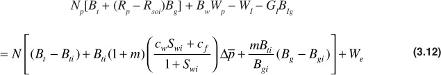
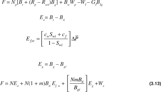
The terms WI (cumulative water injection), GI (cumulative gas injection), and BIg (formation volume factor of the injected gas) have been added to Eq. (3.7). In Havlena and Odeh’s original development, they chose to neglect the effect of the compressibilities of the formation and connate water in the gas cap portion of the reservoir—that is, in their development, the compressibility term is multiplied by N and not by N(1 + m). In Eq. (3.12), the compressibility term is multiplied by N(1 + m) for completeness. You may choose to ignore the (1 + m) multiplier in particular applications. Havlena and Odeh defined the following terms and rewrote Eq. (3.12) as
In Eq. (3.13), F represents the net production from the reservoir. Eo, Ef,w, and Eg represent the expansion of oil, formation and water, and gas, respectively. Havlena and Odeh examined several cases of varying reservoir types with this equation and found that the equation can be rearranged into the form of a straight line. For instance, consider the case of no original gas cap, no water influx, and negligible formation and water compressibilities. With these assumptions, Eq. (3.13) reduces to
This would suggest that a plot of F as the y coordinate and Eo as the x coordinate would yield a straight line with slope N and intercept equal to zero. Additional cases can be derived, as shown in Chapter 7.
Once a linear relationship has been obtained, the plot can be used as a predictive tool for estimating future production. Examples are shown in subsequent chapters to illustrate the application of the Havlena-Odeh method.
1. Ralph J. Schilthuis, “Active Oil and Reservoir Energy,” Trans. AlME (1936), 118, 33.
2. L. P. Dake, Fundamentals of Reservoir Engineering, Elsevier, 1978, 73–102.
3. D. Havlena and A. S. Odeh, “The Material Balance as an Equation of a Straight Line: Part I,” Jour. of Petroleum Technology (Aug. 1963), 896–900.
4. D. Havlena and A. S. Odeh, “The Material Balance as an Equation of a Straight Line: Part II—Field Cases,” Jour. of Petroleum Technology (July 1964), 815–22.
5. L. D. Woody Jr. and Robert Moscrip III, “Performance Calculations for Combination Drive Reservoirs,” Trans. AlME (1956), 207, 129.
6. Sylvain J. Pirson, Elements of Oil Reservoir Engineering, 2nd ed., McGraw-Hill, 1958, 635–93.
7. Denton R. Wieland and Harvey T. Kennedy, “Measurements of Bubble Frequency in Cores,” Trans. AlME (1957), 210, 125.
8. Charles A. Hutchinson, “Effect of Data Errors on Typical Engineering Calculations,” presented at the Oklahoma City meeting of the AlME petroleum branch, 1951.
9. A. F. van Everdingen, E. H. Timmerman, and J. J. McMahon, “Application of the Material Balance Equation to a Partial Water-Drive Reservoir,” Trans. AlME (1953), 198, 51.