CHAPTER 13
Selecting Direct Lending Managers

There is no passive option in direct lending; it is only accessible through active management. It is a dynamic market as managers continuously originate and refinance middle market corporate loans every three to five years, mirroring the private equity market but with greater velocity. The Cliffwater Direct Lending Index captures the collective (asset weighted) work product of the direct loan managers represented in the Index, but it is not investable. Manager selection, therefore, is part of investing in direct loans.

Not surprisingly, some managers have produced better outcomes than others, and by wide margins. The purpose of this chapter is to explore the factors that differentiate direct loan managers and offer suggestions on what characteristics best typify managers who will be successful. But before proceeding, a brief case study is presented to illustrate the importance over time from selecting the right manager.

SELECTION MATTERS

Exhibit 13.1 provides actual loan performance from two of the earliest and largest direct‐lending managers for the September 30, 2004, to December 31, 2017 period. Both manager track records are audited and included in the Cliffwater Direct Lending Index (CDLI).

EXHIBIT 13.1 Performance comparison of two direct lending managers.

Exhibit 13.1 shows clearly that not all managers are alike when executing a direct lending investment program. A dollar invested with loan manager A at September 30, 2004 would have grown to $5.41 as shown in the Total Return line, representing a 13.59% annualized return, gross of fees, and unlevered. Manager A's 13.59% asset performance is also 3.89% above the 9.70% return for the CDLI (see Exhibit 2.1), indicative of significant skill at direct lending. Also impressive is that the 3.89% excess return did not all come from yield. Manager A's income return grew to $4.66, a 12.32% annualized income return compared to 11.15% for the CDLI. A yield difference of 1.17%.

Manager A is unusual in their ability to generate realized gains over this period when direct loans almost always incur realized losses from defaults. Manager A produced these realized gains primarily through acquisition of secondary pools of direct loans at discount during periods of distress, like the great financial crisis (GFC), and a strong record of low credit losses on directly originated loans. While the CDLI incurred realized losses equal to −1.05% over this period, manager A produced realized gains equal to 1.51%, or an excess return from realized gains equal to 2.56% (1.51% minus −1.05%). The 2.56% is the realized gross‐of‐fee alpha produced by manager A.

Unrealized losses were the same for manager A and the CDLI over the measurement period, both equal to −0.33%. Therefore the 3.89% annualized difference in total return between manager A and the CDLI can be divided into 1.17% from excess yield, 2.56% from excess realized gains, 0.33% from excess unrealized gains, and a residual 0.16% that is attributable to both excess yield and gains that represent reinvestment of excess returns. (The 0.16% is often referred to as a cross‐product term.)

Manager B is a completely different story, underperforming the CDLI in both income generation and realized losses.

A dollar invested with manager B at September 30, 2004 would have grown to $2.53, less than one half of manager A, and representing an 7.27% annualized return, gross of fees, and unlevered. Manager B's 7.27% asset performance is 2.43% below the 9.70% return for the CDLI, reflecting poor past performance coming from large realized losses that were not offset by higher income. In fact, manager B's income return of 11.03% was about the same as the CDLI income return of 11.15%, but it realized losses equal to an annualized −3.90%, and well above the CDLI –1.05% realized loss return. A reasonable expectation is that yield and realized losses are inversely related, with investors getting rewarded in higher yields for higher credit risk. That was certainly not true for manager B. Manager B's performance record does show a very small unrealized gain at period's end but clearly the 2.43% total return shortfall to the CDLI is virtually all attributable to poor underwriting that translated into large realized credit losses.

This example demonstrates that manager selection matters, and sometimes a lot. Accepting that, what should an investor look at when selecting a direct lender? For example, should investors just select direct lenders that offer the highest yields? After all, a higher yield would give the investor at least a better starting point, absent any other information.

MANAGER DIRECT LOAN YIELD

Direct lending returns are driven by three primary factors: yield, credit losses, and fees. Yields attract the most attention when evaluating direct lenders because they are an overwhelming source of return, easily calculated, and always available.

Exhibit 9.1 showed that investors hunting for yield can fall into a yield trap, because absolute direct loan yields vary by the types of risks taken. At any point in time investors shopping for yield will find a range of yields being generated by direct loan managers. Exhibit 13.2 reports yield variations across BDC managers for their underlying assets for years 2005 through 2017. Yield is calculated by dividing interest income for the year and dividing that by average gross assets. Each dot represents a different direct lending manager.

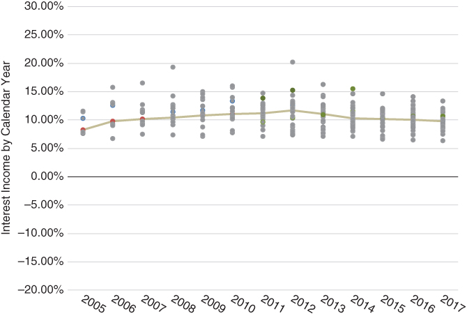
EXHIBIT 13.2 Yield (interest income) by direct loan manager, 2005 to 2017.

Casual inspection of Exhibit 13.2 suggests that both the level and dispersion of manager loan yields remain stable over time. The number of managers represented in the sample grows over the 12‐year period with the growth in new direct loan managers and the number offering BDCs. The asset‐weighted average is shown as a line and represents CDLI interest income.

The dispersion of yields is measured by standard deviation each year. It averages 2.48% over the entire time period but with a higher 3.00% average value over the 2008–2010 period and a lower 2.01% over the most recent three years.

The dispersion in manager yields is best understood by combining the risk premium architecture presented in Exhibit 9.1 with actual direct loan manager exposures to risk factors, as shown in Exhibit 13.3. The diagram illustrates the variation among managers in exposures to risk factors at a single point in time. These manager risk factor exposures remain roughly constant over time, reflecting each manager's preferred style of loan origination. Each bubble represents a single manager and the number is only for identification purposes. The size of each bubble is not a risk factor but measures direct loan assets under management.

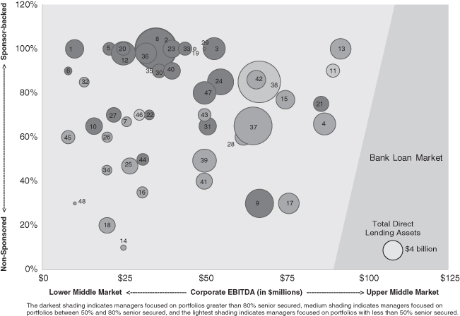
EXHIBIT 13.3 Manager exposure to direct loan risk factors, at December 31, 2017.

The horizontal axis measures the average size of the borrower in the manager's portfolio. This is the fourth risk factor identified in Exhibit 9.1. Size is measured by EBITDA and ranges up to $100 million, which is broadly considered the upper end of the US middle market. Beyond $100 million in EBITDA, borrowers generally access the broadly syndicated bank loan markets for financing. Note the wide dispersion in average borrower size across direct loan managers, with roughly equal numbers of managers operating at different size strata. Also, there does not appear to be a relationship between the size of manager and average size of borrower. Often, investors are concerned that as managers grow in assets they are forced to do bigger deals. While this tendency is found in other asset classes, it has yet to materialize in direct lending.

The vertical axis in Exhibit 13.3 measures manager average exposure to sponsor or non‐sponsored borrowers, the third risk factor identified in Exhibit 9.1. Unlike the symmetric distribution of borrower size, the distribution of sponsored and non‐sponsored exposure favors sponsored borrowers with an average overall exposure to sponsored borrowers equal to roughly 70%. There also appear to be more managers lending to sponsored borrowers and for those lenders to be larger. Lenders to non‐sponsor borrowers frequently point out the increased time and effort required to underwrite their loans. If true, then it would be logical to expect fewer assets and managers doing non‐sponsored loans.

Perhaps most noticeable is the smaller number and size of direct lenders operating in the non‐sponsored lower middle market. This would mean that many managers are purposefully foregoing the full yield premiums found in smaller non‐sponsored loans. This likely is attributable to the ability of asset managers to scale their businesses without smaller non‐sponsored loans.

The last risk factor from Exhibit 9.1 is credit risk and is measured in Exhibit 13.3 by the shading of the bubble. Lenders focused on senior loans have the darkest shading. Lenders making primarily subordinated loans have the lightest shading. Lenders with a broad mix of senior and subordinated loans have medium shading. By number, managers making mostly senior loans and those that invest in both senior and subordinated debt are roughly equal. Only a few managers focus exclusively on subordinated debt, probably because the availability of subordinated debt is less predictable, less scalable, and lenders will also find themselves competing with hedge funds and other special situation managers for these borrowers.

The middle market yield potential measured by the risk premiums in Exhibit 9.1 measured 8.5% (2.6% non‐sponsor premium, plus 2.4% lower middle market premium, plus 3.3% subordinated premium) at December 31, 2017. The actual range in middle market yields, from high to low, offered by direct lending managers equaled 7.6% for the same date shown in Exhibit 13.2. Excluding the highest and lowest yielding managers, the dispersion in return equaled 5.7%. This variation in yield among direct lenders is significant but largely explained by risk factor exposures by those managers. The regression of manager risk factors and yields produced an R‐square equal to 0.75, meaning that 75% of the variability in manager yield is explained by the risk factors. Combining the 75% R‐square between yields and risk factors with the 2.01% cross‐sectional standard deviation in yields over the past three years implies that the standard deviation of yields across direct lenders not explained by risk factors equals a smallish 1.01%.

It appears that direct lenders have limited ability to affect yield in a significant way except by taking on factor exposures rewarded by high‐yield premiums. And it is likely that the 1.01% dispersion not explained by risk factors are created by differences in the extent to which managers self‐originate loans, earning original issue discount fees (OID) versus participating in smaller or larger club deals and receiving partial or no fees. Another explanation is that some direct lenders engage in an industry focus, such as venture or healthcare lending, which have higher asset volatility and therefore higher yields, as explained in Chapter 8.

In the broader credit markets, and for the direct lending market as well, the level of interest income (yield) likely represents beta. In most cases differences in yield can be explained by the major risk premiums identified in Chapter 9 or other factors unrelated to manager skill. In the market for financing, even in the middle market, there are sufficient competitive pressures among lenders that yield anomalies would seem hard to come by.

CREDIT LOSSES ACROSS DIRECT LENDERS

Risk premiums provide a very useful explanation for the different yields found in US middle market direct lending but there is not sufficient evidence that they are useful in explaining credit losses, the second component in direct lending returns. Instead, the variability in realized credit losses appears thus far to fall at the footsteps on the lender itself and its underwriting capability.

Exhibit 13.4 parallels Exhibit 13.2. In Exhibit 13.4 realized credit gains (losses), rather than interest income, are shown by calendar year for individual direct lending managers together with the CDLI, which represents an asset‐weighted average. Scaling is identical for both Exhibits so that visual comparisons are not misleading.

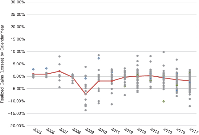
EXHIBIT 13.4 Net realized gains (losses) for direct lending managers and the Cliffwater Direct Lending Index, by year.

Dispersion among manager realized gains (losses) in Exhibit 13.4 is significant and exceeds differences found for interest income. The average annual cross‐sectional standard deviation of realized gains (losses) equals 3.61% for the entire period and rises to 4.94% during the 2008–2010 subperiod when losses from the GFC were realized. By contrast, the cross‐sectional standard deviation in interest income was 2.38% for the entire period and 3.00% during the 2008–2010 GFC subperiod. Statistically speaking, an investor focus on a lender's ability to manage credit losses is significantly more important than their ability to generate interest income. Statistically speaking, managing credit losses is 2.3x more important than income generation, calculated by the ratio of variances (the square of standard deviation).

The 3.61% cross‐sectional standard deviation in realized gains (losses) across direct lending managers is very meaningful, considering that the standard deviation CDLI returns over time is 3.5% (Exhibit 3.1). This is not like traditional stocks and bonds where active manager risk (alpha risk) is a very small percentage of overall market risk (beta risk). In direct lending, individual manager risk can exceed the risk of the direct lending asset class itself.

Exhibit 13.5 presents realized gains (losses) in another way by showing cumulative net realized gains (losses) by direct loan manager. The length of track record varies across managers with many starting after the GFC. As a result, Exhibit 13.5 contains track records of net realized gains (losses) of differing lengths. The heavy dark line represents aggregate CDLI net realized losses. However, the graphic is useful in showing the long‐term dispersion of realized gains (losses) across managers and not just yearly dispersion.

EXHIBIT 13.5 Cumulative net realized gains (losses) for direct lending asset managers and the Cliffwater Direct Lending Index (heavy dark line): September 2004 to December 2017.

A key question is whether the risk factors that explain so much of the differences in direct lending interest income among managers also explain differences in manager realized credit gains (losses). Finding an answer that is statistically meaningful is difficult because realized credit losses are concentrated over just a few years, 2008–2010, covering a small sample set of direct lenders. Most of the remaining years are largely credit benign with little or no credit losses. In those years differences in portfolio yield may reflect perceived risk of default, but without actual defaults a statistical relationship won't be found.

The correlation between calendar year interest income and realized credit gains (losses) equals −0.11, suggesting that higher yield direct lending portfolios tend to experience lower realized credit gains (larger realized credit losses). Assuming higher yields reflect greater credit risk, the negative correlation is directionally correct. However, the R‐square equals just 1% meaning that for all practical purposes there is no relationship between yield and credit losses that can be gleaned from the historical data.

These results leave one of two possibilities. Either yield does forecast credit risk but there is not sufficient data yet to support it, or credit loss differences are better explained by differences among direct lenders in their skills at sourcing, underwriting, and workout capabilities. Of course, both yield and manager underwriting may explain credit loss outcomes.

TOTAL RETURN

Historical data on yield and credit gains (losses) suggest that direct lender performance can vary widely across managers. Yields vary widely across direct lenders given their exposure to risk factors and realized credit losses vary widely due to differences in underwriting skills. And the lack of correlation between yield and credit loss increases the dispersion of manager returns, rather than reducing it. A wide dispersion among direct lenders in calendar year total return (incorporating yield, realized gains (losses) and unrealized gains (losses)) is indeed found in Exhibit 13.6.

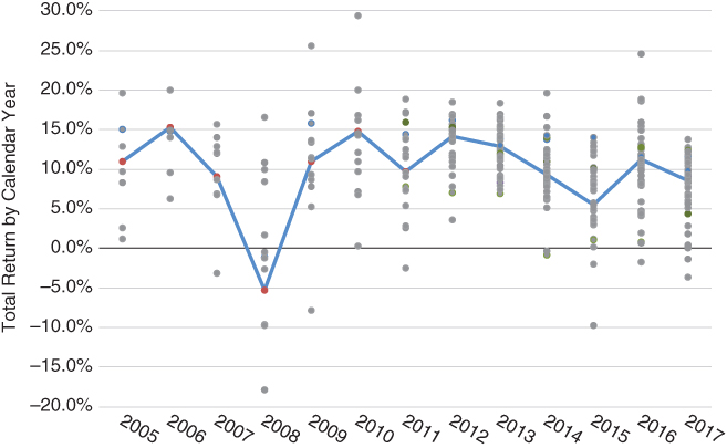
EXHIBIT 13.6 Total return for direct lending managers and the Cliffwater Direct Lending Index, by year.

The average cross‐sectional standard deviation of return equals 6.58%, which is high for asset classes, with the exception of private equity, and has implications for portfolio construction discussed in a later chapter. A major takeaway from this dispersion analysis is that the selection of direct lending managers is very important and that the risk found in manager selection likely exceeds the risk found in the asset class itself. This means that the common approach of hiring a single manager to gain exposure to direct lending and then adding managers as allocations increase probably presents unnecessary risks. It is better to hire several direct lenders at the outset to get a better chance of replicating asset‐class characteristics.

DIRECT LENDING MANAGERS

Direct loans are bespoke agreements between lenders and borrowers. As such, successful investment outcomes are dependent upon the quality of the direct lending manager(s) selected by the investor.

Unlike just five years ago, investors today have a variety of asset‐management firms to select from. The population of direct lending managers has grown rapidly since the GFC and continues to expand in line with the growth in direct lending assets. Unlike many other traditional and alternative asset classes, there has yet to appear any significant concentration in assets among a few firms. At December 31, 2017 there were roughly 225 global direct lending firms, 160 located in the US. These firms combined managed $270 billion in direct lending assets globally, with $205 billion in the US and $60 billion in Europe. Direct lending in Asia is in its infancy with perhaps a dozen managers investing $5 billion in direct loan assets.

An institutional approach to selecting a direct lender likely involves a multifaceted analysis, such as the one described in Exhibit 13.7. Like most other asset classes, a small minority, perhaps 20% of available managers, meet the highest qualifications and fiduciary standards. There is generally another group of 20–30% that are of institutional quality but lack a few characteristics that put them in the highest grouping. Finally, roughly 50% or more available managers are unlikely to produce good outcomes due to multiple deficiencies.

EXHIBIT 13.7 Due diligence checklist for middle market direct lender.

ORGANIZATION

Successful money‐management firms have experienced investment and operational personnel with good resources at their disposal. Ideally, the investment people have been working together under one roof for a long period of time. But for a few managers, many direct lending organizations have been newly formed over the past 10 years and thus don't have long histories. In those cases, the professional team may have worked together at a bank or nonbank financial lender prior to the GFC and were recruited to a asset management firm or started a new firm during the GFC. This in fact was a common scenario in direct lending, at least in the US. Many successful direct lending professionals today have pedigrees going back to pre‐crisis, including nonbank commercial lenders such as GE Capital and CIT. Others came from commercial banks such as Continental, First Chicago, Fleet, and the NY investment bank proprietary trading desks. These professionals were well trained and experienced in middle market corporate lending well before direct lending became popular.

Operations has a critical role to play at any direct lending organization. Unlike stock and bond managers, where every security has a digital identifier with terminal access to all sorts of data and a great number of operational functions are outsourced, most direct lenders deal with loan documentation and terms that require identification, measurement, and compliance that is not available off‐the‐shelf. While some functions can be outsourced to capable vendors, this does not change the need for the direct lender to input data, feed it to the vendor, and verify accuracy. Several of the early direct lending firms built their own administrative systems for lack of good off‐the‐shelf products. That is one reason administrative expenses for operating a direct lending portfolio can be high, up to 0.40%, though the average is around 0.20%.

INVESTMENT STRATEGY

Most direct lending managers have a similar investment strategy: maximize interest and other income and avoid losses from defaults. They can differ greatly in how they execute, and that is where lenders are differentiated. Borrower type and size are the most significant differentiators, as described in Chapter 9. Many direct lenders deal only with borrowers backed by private equity sponsors. Here, the number and depth of these relationships with private equity firms is very important and can be verified through reference checks. It is also useful to know the reputation of the private equity firms, particularly in dealing with their portfolio companies during downturns.

Only a few asset managers lend exclusively to non‐sponsored borrowers. More often a direct lender will source both sponsor and non‐sponsor borrowers. Yields are higher for non‐sponsor loans but lenders also need to consider the slower rate at which loans can be made and longer effective maturity due to a lower chance of prepayment. In both cases they are likely much slower. For example, non‐sponsored companies are likely to have fewer corporate actions (liquidity events).

Direct lenders typically differentiate themselves into lower middle market, middle market, and upper middle market. The lower middle market would be borrowers with EBITDA less than $25 million while the upper middle market are borrowers above $75 million in EBITDA. Lender focus is usually based on existing sponsor relationships or other sourcing avenues. Lenders in the upper middle market need to guard against excesses, like covenant lite, that merge from the broadly syndicated bank market to the upper middle market for direct loans. Lenders in the lower middle market see more stable borrower metrics and terms, but need to pay more attention or allocate more resources to problem loans and exit strategies.

Lenders will also differentiate by the level of credit risk taken. Some are senior secured only while others look at the totality of the business they are lending to and may lend at several levels, including subordinated. Unitranche lending, which combines senior and junior loans so that the lender becomes a single turnkey source of financing for the borrower, is rapidly growing in popularity. To be successful, unitranche loans need to be priced lower than the typical senior/junior debt structure. The positive is that investors may get more money to work with unitranche lenders, but the negative is that the investor may give up yield for the risk taken.

A smaller group of direct lenders focus on certain industries. Healthcare and technology (venture) lending are two examples. These lenders take advantage of the higher yields (beta) offered by these higher risk industries and seek to mitigate risk of default (alpha) through specialized industry expertise.

ORIGINATION

Direct lenders originate loans, but not entirely. The classic direct lender sources loan deals, structures the loan documentation, holds the entire loan to maturity and likely after financing, monitors the borrower for covenant compliance and works out the loan in the case of borrower distress. For sourcing and structuring, together called origination, the direct lender receives compensation in the form of deal fees that are paid up front or original issue discount that, while accounting treatment can vary, is usually amortized as income over the life of the loan.

Roughly 20% of the direct lenders today are of the classic variety described above. Another 70% may self‐originate but can also participate in small club deals, where a few direct lenders agree to participate jointly in a loan pari passu. In these cases, the club may be formed because the loan is too large for the direct lender who found the deal, or that lender might invite other lenders to diversify into more loans as other club members reciprocate. With smaller clubs, deal fees are shared but not always equally. Finally, less than 10% of direct lenders do not originate deals but lend only through participations from large lead arrangers like a GE Capital. These direct lenders effectively outsource the origination process. Their loan portfolios forego the extra income, but they are typically much more diversified by number of loans and industry. While origination sounds great and produces extra income and perhaps an informational advantage relative to borrowers, it also can present a bottleneck to the investment opportunity set that can frustrate portfolio construction and risk management.

Most direct lenders organize origination and underwriting functions together around industry verticals. There are exceptions where the origination team operates independent of the underwriting team, a model traditionally found in commercial bank lending. The move to combining these functions is likely due to the need for speed of execution and the ability to bring industry expertise to the borrower early in the engagement.

UNDERWRITING

In theory, underwriting is the process of structuring financing to fit the needs of the borrower while at the same time assessing risk. Risk assessment includes the concepts of expected default frequency and recovery given default. Expected default frequency addresses the size of the loans relative to firm assets and cash flow to minimize the future probability of a default happening. Recovery given default refers to having sufficient security so that if default occurs there is an opportunity for full recovery of loan proceeds.

In practice, borrower financials and proposed loan amounts are used by the loan manager to determine implied credit ratings or shadow ratings based upon comparisons provided by the major rating agencies. For example, loan leverage levels (loan to EBITDA) for the proposed loan at issuance is compared to equivalent measures determined by rating agencies for different quality grades, from single A to CCC. The proposed loan is given a shadow rating that best matches its leverage level at issuance. In turn, the shadow rating is used to set pricing (yield) based upon what the loan market is currently offering for that shadow rating.

Underwriting is generally performed by the industry specialist, whose work is then reviewed more broadly by an investment committee.

Of course, loan managers consider many financial variables, not just leverage levels, in their mapping of a specific loan to a rating agency's letter rating. Hence, the loan manager is basically rating the loan, not the rating agency. But loan managers generally rely on rating agency letter grades to accurately reflect risk. Market yields for each rating then sets the price for accepting a given assessment of risk.

LOAN CONSTRUCTION AND MONITORING

A general discussion on loan agreements and covenants is in Chapter 10. Direct lenders use the underwriting process to settle on loan terms and covenants that will be required to finance the borrower. In most cases direct lenders use the services of outside law firms that specialize in structured finance to assist in constructing and negotiating loan terms. Compliance with the loan agreement requires ongoing monitoring of borrower financials. Most loans have maintenance covenants that require periodic (quarterly) collection of data from the borrower and covenant testing.

WORKOUT

The final step of the investment process is the workout of the loan in case a default occurs. Oftentimes, the default is technical and requires the borrower to pay a fee or greater interest rate as remedy. In situations where there is an actual default stemming from a fundamental problem with the borrower the lender will need specialized expertise and resources to maximize recovery value. Not all direct lenders have these skills. Some direct lenders operate as part of larger alternative asset management firms that include private equity and distressed capabilities. These direct lenders are better positioned to handle the recovery process versus the alternative of a distressed sale.

PORTFOLIO CONSTRUCTION

The most common vehicle for investing in corporate direct loans is a private partnership with a limited life. Asset managers that construct portfolios of direct loans for private partnerships seek to optimize return and risk, subject to the level of committed assets, the period of time designated for investment, and the deal‐flow opportunity during the investment period. Like private equity, most investors in direct lending will have concurrent commitments to more than one direct lending manager because no single manager can optimize the entire direct lending opportunity set. Understanding this, the direct lender should optimize its own opportunity subset and let the investor optimize the full direct lending opportunity through multiple managers. This design has worked well for institutions investing in private equity and private real estate.

EXHIBIT 13.8 Portfolio characteristics for direct lending private partnerships.

67	Number of private partnerships represented
13	Number of vintage years represented
$37 billion	Gross assets represented
$255 million	Median fund commitments
$455 million	Median fund gross assets
0.70x	Median leverage as % of NAV
9.37%	Net IRR
0.20%	Median realized credit loss ratio (annualized)
$29 million	Median borrower EBITDA
$44 million	Asset‐weighted borrower EBITDA
4.48	Median loan leverage (debt as % of EBITDA)
81%	Average % sponsor‐backed loans
72%	Asset‐weighted, sponsor‐backed loans
47	Median # of loans
66%	Median % senior secured
68%	Asset‐weighted % senior secured

Understanding that they will not be responsible for investors' overall market diversification (beta), direct lenders instead maximize the yields they can manufacture while minimizing credit losses (alpha). Investors will commit to several direct lending funds of complementary strategies to optimize their overall allocation to direct lending. But direct lenders don't always agree on this view of portfolio construction. Some design their portfolios to be more turnkey, believing their investors want to one‐stop their direct lending exposure. These managers generally have been in business longer and have investors that may have relied principally on one manager. Other managers have very focused direct lending strategies with a greater emphasis on return maximization and who should represent one component of an overall direct lending allocation.

Exhibit 13.8 provides some general statistics on private partnerships investing in direct corporate loans over the last 15 years. These statistics should provide some guidance on how actual portfolios are constructed.

The portfolio statistics for the sample of private partnerships are not dissimilar from BDCs. This should not be too surprising because many asset managers offer both private partnerships and BDCs. Noteworthy is the 0.70x median leverage, which is very similar to the value found in BDCs, whose leverage was constrained by regulation to 1.0x until recently. If investors select partnerships with an average leverage ratio below 1.0x, from a risk perspective they may not prefer BDCs that now ramp up leverage close to the 2.0x maximum now allowable.

The median number of loans is 47, which is adequately diversified for a single fund but probably not for an investor, particularly when leverage averages 0.7x. That means that the average position size, as a percent of NAV, equals 3.6%. One default, with an offsetting 60% recovery rate, would lower the internal rate of return (IRR) of the private fund by roughly 30 basis points over its five‐year life. Given that loans have limited return upside, most investors would want to have broader representation of credits through multiple funds.

The 0.20% realized credit loss ratio stands out compared to the 1.05% realized credit losses reported for the Cliffwater Direct Lending Index. The low loss ratio for the private funds is largely attributable to the sample set that consists of many more post‐GFC funds (61) when credit losses were lower compared to pre‐crisis funds (6).

It is important to understand the portfolio construction strategy for any individual loan manager and how it fits into an investor's overall portfolio.

LEVERAGE FINANCING

Most middle market direct lenders enhance yields by using a modest amount of leverage, ranging from none to 3.0x. The higher levels of leverage are used for the most conservative middle market credits while portfolios of subordinated and mezzanine loans use little or no leverage. As reported above, the average BDC and private partnership generally operate with leverage between 0.5x and 1.0x.

There are several methods for financing asset purchases, each with pros and cons. The first is the subscription line. These credit facilities have recently become very popular where banks will lend BDC or private partnerships against their undrawn committed capital. Consequently, subscription lines are a temporary source of financing, existing only until committed capital is fully drawn by the general partner. The amount of bank financing under the subscription line depends upon several factors, including the size of the fund and the creditworthiness of investors. Subscription lines are relatively cheap, priced at 1.50–1.75% over Libor, but like revolving loans, the lender pays an unused commitment fee, typically 0.25%. Subscription lines are very useful early in a fund's life when the portfolio is being ramped up and does not have the diversification necessary to satisfy asset‐based lenders. Subscription lines have also become a popular way to boost the IRR calculation of performance since income is generated on little to no net asset value. On the other hand, some investors have gotten frustrated with a manager's borrowing on uncommitted capital rather than just calling capital because the undrawn commitments may be held by the investor in reserves that are earning less than the financing costs of the subscription line.

The second and most common financing method is for the direct lender to enter into an agreement to create a revolving credit facility. The facility provides the direct lender financing as needed (revolving) subject to limits. The financing is provided by multiple parties, typically banks, arranged by a syndication agent, and guaranteed by the underlying portfolio of loan assets. The revolving credit facility is generally costlier with a 2.25% to 2.50% spread over Libor and a 0.375% charge on unused amounts. But unlike a subscription line, the revolver is a more permanent source of financing with a four or five‐year maturity.

A third financing method is the creation of a special purpose vehicle (SPV). SPVs are lending vehicles, also with four or five‐year maturities, secured by loans placed in the SPV. Costs tend to be somewhat higher than revolvers at a 2.50–3.00% spread over Libor. They also tend to be more manually intensive. There are many types of SPV facilities, including the availability of term financing, flexibility in asset level approvals, and the ability to use them as warehouse financing for CLO take‐outs, or for rated structures.

A fourth financing source, and one more commonly found in permanent capital structures like BDCs, is longer maturity (5+ years) unsecured and subordinated notes issued in private placements or through public offerings. These generally have fixed rates at higher costs. A few managers have entered an interest rate swap matching floating‐rate to fixed‐rate payments. On a swap‐adjusted basis the financing might cost a little more, but it is very flexible and easy to support compared to SPV facilities, which can require significant resources.

A fifth source of financing can come from the Small Business Administration (SBA). The SBA was established in 1958 by Congress to stimulate small business growth and, today, is responsible for roughly $25 billion in loans to small businesses. Direct lenders can access SBA financing by getting licensed by the SBA to set up a Small Business Investment Corporation (SBIC). The SBIC is akin to a private partnership where the direct lending asset manager is the general partner and institutional investors are limited partners. SBICs are attractive to its investors – general and limited partners – because they can issue SBA‐guaranteed debentures at 10‐year maturities, with no principal amortization, at favorable interest rates compared to other traditional sources of financing, and at levels up to 2.0x investor capital. However, SBA financing is limited to $150 million per SBIC and $350 million for multiple SBICs under a common manager. SBICs must also direct their loans or other investments to qualifying companies, which are generally smaller middle market companies with EBITDA less than $10 million or companies in industries or sectors designated by the SBA for favorable treatment.

Understanding how direct lending managers arrange their sources of financing, how cash flows from loan assets match the interest and principal repayment requirements of credit facilities, and how financing costs are optimized across the potential sources, are critical components of investor due diligence.

FEES AND EXPENSES

Chapter 15 discusses manager fees in some detail. Fees have generally been coming down as they have in most other asset classes. Part of the reason in direct lending is asset growth has allowed managers to reduce costs as increased scale has widened operating margins. Also, the entry of institutional investors has brought greater attention to both the level and structure of manager fees. But not all direct lenders have the same strategy and more labor‐intensive strategies will continue to charge higher fees.

TRACK RECORD

The lack of a track record history through the GFC has been a hindrance to evaluating many of the direct lending firms formed over the past 10 years. A few direct lenders do have track records that extend well before the GFC and are generally able to provide sufficient granularity to decompose returns into income, realized losses, and unrealized losses. Direct lenders that operate BDCs are required to provide this detail to shareholders, so the information is readily available and verifiable. Detailed performance data from direct lenders that do not operate BDCs is often not available from the manager. This is because direct managers generally follow the performance practices of their private equity brethren and only report total net performance by fund, by vintage year. Unfortunately, it is impossible to glean information on a lender's credit‐loss experience from a performance presentation of this type. Without changing their reliance on IRR, more direct lenders are now supplementing performance disclosures with default and recovery histories.

In the case of direct lenders formed after 2008, an understanding of their abilities during downturns requires parsing performance histories at prior firms, which is more difficult. Nonetheless, the investor can generally come to some conclusion as to whether the current team or its individual members successfully navigated the GFC. That said, there is nothing better than actual, audited returns during a downturn to verify underwriting and workout capabilities.