The present volume is based on reported, recorded, and observed data which we have accumulated in the course of the last fifteen years. As in our previous volume on the male, the reported data have been derived from case histories secured in personal interviews. The recorded data have included sexual calendars, diaries, personal correspondence, scrapbook and photographic collections, artists’ paintings and drawings, and still other documentary material supplied by a series of our subjects (Chapter 3 ). Observations of sexual behavior in fourteen species of mammals, and clinical material supplied by a long list of medical consultants, have been the chief sources of the observed data (Chapter 3 ).
Over the course of the past fifteen years, 16,392 persons have contributed their histories to this study. To date, we have secured the histories of 7789 females and of 8603 males. Our more general information and thinking on female sexual behavior are based on this entire body of material, even though the statistical analyses have been restricted to a portion of the female sample. Because the sexual histories which we have of white females who had served prison sentences (915 cases) prove, upon analysis, to differ as a group from the histories of the females who have not become involved with the law, their inclusion in the present volume would have seriously distorted the calculations on the total sample. Neither has the non-white sample (934 cases) of females been included in the calculations, primarily because that sample is not large enough to warrant comparisons of the subgroups in it. The statistical analyses in the present volume have, therefore, been based on our 5940 cases of white, non-prison females. In order to standardize the statistical calculations, histories acquired since January 1, 1950, have not been used.
The 5940 females whose histories are statistically analyzed in the present volume represent something of the great diversity which exists among American females. Certain groups are well represented in the sample, and the conclusions based upon the data which we have obtained from those groups may, with some warrant, be extended to the comparable portions of the total American population. Certain other groups are not so well represented in the sample, and we cim make no prediction at the present time as to the behavior of those portions of the population. A description of the sample which has been used in making the present volume, some discussion of the problems of sampling in general, and a discussion of some of the specific problems that have been involved in securing a sample for this study of human sexual behavior, are among the subjects contained in the present chapter.
Functions of a Sample . It should be emphasized that most of our everyday generalizations concerning matters which pertain to more than a limited number of individuals or specific circumstances are based upon some sort of sampling, since it is usually impossible to measure each and every individual in any large group before one attempts to generalize concerning the characteristics of the group. Everyday experience has taught all of us that an acquaintance with a smaller number of individuals may, within limits, give us a practical understanding of the larger group.
The ideas which most persons have concerning the sexual attitudes and behavior of the population as a whole are, for the most part, based upon their own personal experience, on fragmentary information picked up from contact with a relatively small number of friends, on newspaper and magazine reports, or on more general gossip. Our everyday knowledge of the capacities of the utensils and tools that we use, our likes and dislikes for particular kinds of food, the confidence or fear with which we cross a street in the face of moving traffic, our evaluations of our acquaintances and friends, and most of the other generalizations by which we live, are based upon a limited number of experiences which, nevertheless, most persons consider sufficient to warrant the generalizations which they draw.
Probability Sampling . The problem of securing a sample that may adequately represent the larger population from which it is drawn, has long been recognized. Innumerable systems have been devised for the selection of the individual elements that go into a sample, ranging from the casting of lots, the shaking up of slips of paper in a hat, the shuffling of a deck of cards, the tossing of coins, and the use of a roulette wheel, to the most refined methods of modern probability sampling. The basic concept of a probability sample involves the development of some method of selection which allows each individual in the population a known chance of being selected as a part of the sample, without the introduction of a bias which might lead to the inclusion of particular types of individuals more frequently than they occur, proportionately, in the population as a whole. Various modifications of simple, unrestricted sampling, such as stratified and still other types of sampling, are frequently employed without, however, changing the basic concept that lies back of all probability sampling. 1
The selection of a probability sample usually begins with a listing of all the units, such as the dwelling units, the city blocks or the other sections of a city, the rural townships, the institutions, or the other units which make up the total area or universe which is the object of the study. Sometimes a published census or a city map or directory or some previous survey may provide the necessary information; sometimes a preliminary survey must be made by the investigators themselves. On the basis of the preliminary census, certain of the units are then selected by some mathematically controlled system of randomization, and the selected units are then intensively studied, or individuals from each of the selected units are chosen, again by an impersonal and mathematically objective process, for special study. After the selection of the sample, the problem becomes one of locating the chosen individuals and persuading them to cooperate. If the survey involves more than a few questions, there is the problem of persuading the interviewee to give sufficient time to the interviewer; and if the material covered by the survey has any considerable emotional significance, as in a study of sexual behavior, the interviewer’s success will also depend upon his skill in getting the subject to frankly, fully, and freely contribute the desired information.
Properly selected, a probability sample should include its proper proportion of each type of individual in the population which is being studied. In a sex study, it should include proper proportions of persons with high levels of sexual activity, persons with low levels of activity, persons whose histories involve only the usual (the predominant) types of behavior, and persons whose histories include the less common types of behavior. The probability that each type of variant in the population will be proportionately represented in the sample will depend, to some extent, upon the size of the sample; and by increasing the size of the sample, the investigator may control the level of approximation which the sample may afford—provided, of course, that the selection of the individuals continues to be on a random basis.
With a probability sample, it should be possible to determine, mathematically, the probable limits of error which would be involved in extending generalizations from the sample to the total population from which it is drawn. This is a matter of very considerable importance, and the one which is primarily responsible for the increasing use of probability samples in government surveys—including the current population studies of the Bureau of the Census, many of the studies of the U. S. Public Health Service, the Bureau of Labor Statistics, the Department of Agriculture—, in some of the state surveys being conducted under university agencies, in some business surveys, and in an increasing number of scientific research studies. 2 The predictive value of a probability sample is of such importance that whenever its use is feasible, and whenever the cost of such sampling is commensurate with the function it may serve, there is good reason for using it in any statistical survey. Nevertheless, we have deliberately chosen not to use a probability sample in the present study of human sexual behavior.
Probability Sampling in a Sex Study . Our first and most decisive reason for not doing probability sampling on the present project has been the necessity for obtaining cooperation from the individuals who have served as the subjects for the study. It has been necessary to convince each individual to give the time necessary for the interview, and to agree to answer questions on matters which many persons have never discussed with anyone, even including their spouses and their most intimate friends. We have asked for a record that was as frank and full and honest as memory would allow.
The problem has been very different from the problem that is involved in random sampling which is done to determine, for example, the incidences of an insect pest in a wheat field, or to determine the occurrence of some physical phenomenon in a group of inanimate objects. It should be obvious that a considerable proportion of the persons selected for study by the objective and impersonal processes of random sampling, and confronted by an investigator of whom they had never heard, would simply refuse to give information on as personal and emotional a subject as sex. Even in surveys which have been concerned with economic, social, or political issues, the refusal rates have often been high enough to cast doubt on the validity of the results. 3 Our experience leads us to predict that the attempt to secure sex histories from lone individuals who were not part of some group with which we were working, would have resulted in refusal rates so high that the sample would have been quite worthless.
Moreover, even among the persons who might have agreed to answer some of the questions, it is certain that many would not have given as full and complete information as we have been able to secure through winning the confidence of the community with which we were working, and then establishing rapport with each individual subject in the community (pp. 28–31, 58–64).
In this, as in many other studies of human populations, the requirements of accurate reporting and accurate sampling are to some extent antagonistic. Somehow one must decide upon a compromise between the two. We have desired neither a representative sample ofunreliable answers, nor a set of reliable answers from respondents who represented nobody but themselves. For this reason we have been compelled to substitute for probability sampling a method of group sampling through which we have tried to secure representatives of each of the components of the larger population in which we were interested.
Our second chief reason for choosing to work with social units rather than with a sample chosen on a probability basis, has been the near impossibility of defining groups which could be sampled by some probability scheme. Since patterns of sexual behavior may be considerably affected by the individual’s age, educational attainment, occupational class, religious background, and other social factors, we have needed samples from groups constituted on those bases; and it would have been very difficult or impossible to have secured any sort of census on a nationwide or even statewide scale which would have allowed us to choose the subjects for probability samples from such groups.
It should be pointed out that we have been concerned with much more than the problem of arriving at a single set of over-all figures on the incidences and frequencies of each type of sexual activity in the total American population. Scientists are more often concerned with analyzing the relationships between the phenomena which they study, than they are in tabulating the incidences of such phenomena. Causal relationships or parallel effects may be discovered by correlating the relative incidences of phenomena in different groups of individuals and their distribution in relation to ecologic, geographic, or other factors. This is what the laboratory biologist does when he compares an experimental group with a “control” group which has not been operated upon or given the special feeding or drugs or hormones which were given to the experimental animals. This is what the taxonomist does when he attempts to analyze the evolutionary origins of the characters of a given species of plant or animal by measuring samples drawn from a variety of localities, or by measuring samples of related species. This is what the geneticist does when he compares the characters of a parental generation with the characters of their offspring, and thereby arrives at generalizations concerning the processes of heredity.
In the present study, it is true that we have been concerned with the incidences of masturbation, of pre-marital petting, of pre-marital coitus, and of various other types of sexual activity; but we have also been concerned with discovering the factors which contributed to the origin, the development, and the social outcome of each pattern of behavior. These things cannot be determined from a simple enumeration of the number (the incidences) of persons having such experience in the total population. Their exposition must depend upon comparing samples from each of the sub-groups in the total population—from groups which differ in their marital status, their educational levels, their occupational and religious connections, and their other social backgrounds.
If we had done any sort of proportionate sampling, it would not have given us adequate samples for analyzing each of these component groups. If, for instance, Negroes constitute only 10 per cent of the total U. S. population, a proportionate sample would have included only one-ninth as many Negroes as whites, and that would have constituted too small a sample for analyses of Negroes, unless we had secured an unnecessarily large sample of whites. It is true that if this had been the only difficulty it could have been overcome by taking equal-sized samples of each group and, wherever an over-all figure was desired, combining each component with an appropriate weight. Thus, in the present instance, an over-all figure could have been obtained by multiplying the Negro data by one, the white data by nine, and dividing the total by ten. Such a procedure, which is quite common, is still probability sampling and still possesses all of its advantages.
But to have secured such a probability sample from each segment of the population would have demanded such years of work and such financial resources as no one has yet proposed to put into a study of human sexual behavior; and while we might have secured better statistical data on the incidences of the various types of sexual activity, we would not have arrived at our present understanding of the other, non-statistical problems which we have considered of equal importance in the present study (see especially Chapters 14 –18 ).
Group Sampling on Present Project . For these several reasons we have chosen to secure the subjects for the present study by working with the various social units to which they belonged. By winning the confidence of each group, we have ultimately obtained the cooperation of its individual members. Individuals in any cohesive group are more willing to contribute when they learn from their friends that such cooperation does not involve undue embarrassment, and when they observe in the course of time that none of their friends have gotten into difficulty because they have contributed. Many persons who, as lone individuals, see no particular advantage in giving their histories, are willing to do so when loyalty to a group project is involved. Thus it becomes more feasible to secure the histories of all members of a group than it is to secure the histories of single individuals chosen at random out of that group. No such group psychology is available to persuade the lone rancher living on the Western plain, the particular Negro in the swamps of Alabama, or the particular youth engaged in underworld activities in the heart of an Eastern city, when they are chosen, by the processes of randomization, as the ones who are to contribute their sex histories to a scientific study.
In principle, of course, it would have been desirable to have drawn a probability sample of the groups with which we wanted to work. But the limitations on the nature of the groups that can be used in a probability sample are so severe as to render them essentially inaccessible. For instance, the groups should be such that any individual belongs to one and to only one of the groups that enters the sample. This would immediately preclude the possibility of working with parent-teacher groups, church groups, sororities, and the like. The groups that best satisfy the ideal are groups that are confined to particular geographic areas. But since neighborhoods, particularly in large urban areas, may be among the least cohesive of all groups in our modem social organization, often involving no group loyalties and no effective means of communication, the problem of securing cooperation from neighborhood groups is sometimes insurmountable.
There are further difficulties in choosing the groups with which one works. It is not always possible, for instance, to secure a census of the individual units of certain groups, such as fraternal or service clubs, colleges of some particular type, parent-teacher organizations, church groups, underworld communities, local community clubs, and various others. Without such a census, the random selection of the particular groups with which one should work is impossible.
Moreover, to have secured the cooperation of a particular group chosen at random would, in many instances, have been as difficult as securing a sample of lone individuals chosen at random. For example, having selected a particular prison at random, the chances of securing entrance to the institution and of securing the necessary cooperation from the administration and inmate body of the institution would have been slight. On the other hand, working first in some institution that had become available through contact with an understanding warden or some state board official, it became possible to get into a second institution, and that in turn, after many years of labor, opened the doors of the very institution which would have barred us if it had been selected in the first place as the lone representative with which we wished to work. Similarly, our entrance into underworld groups has usually depended upon making some lone contact which was cultivated sometimes for months or a year or two before we secured any additional history from the area; but with such slow progress over a matter of two or three years, we finally were able to develop sufficient acquaintance in the community to make any and essentially all of its members accessible for study. We have gone into colleges, into church groups, and into many other groups where we would never have obtained entrance except for their relation to some other group with which we had previously worked. Such a method of choosing groups has undoubtedly introduced biases, but there are more practical difficulties involved in the application of sampling ideals than some theoreticians realize unless they have been faced with the actualities of obtaining data on a subject like human sex behavior.
Nevertheless, it has been possible in some instances to exercise some control over the choice of groups. For instance, in college communities it has been possible in a preliminary general lecture to emphasize the desire to work with groups and not with individuals who might volunteer histories. From a list of a score or more groups that were then suggested, we could choose one fraternity or more, a sorority or two, several student rooming houses, a large cooperative house for non-organized students, the members of a student class or two in the local churches, a student social group, several classes in undergraduate courses, in graduate courses, in summer courses for older adults and professional persons returning for additional study, and still other types of groups. With each of the chosen groups it has then been possible to work intensively until we secured the histories of all the individuals or of a large proportion of all the individuals in each group. While it is still impossible to calculate the probable error on such a sample, it provides a diversification and a representativeness which far surpass that which might have been secured by depending on lone individuals who volunteered to contribute histories.
In a city community or in a rural area, the entrée may be obtained through some single individual, usually some significant individual in the community; but again we have tried to stay with each group until we have won the confidence of the whole community, and until we have obtained the histories of a high proportion of all the persons in the community. In one rural, sparsely settled western area an examination of the tax list showed that we had obtained the histories of 75 per cent of all the males and females in the community above fifteen years of age. In one church community, where less than ten persons had volunteered histories after the initial lecture to the assembled congregation, we ultimately obtained the histories of 180 out of the membership of 220. Most of the others in the group were out of town, ill, or inaccessible for other reasons and not because they refused to cooperate.
In one sense, everyone who has contributed to this study has been a volunteer, for no one can be forced into the disclosure of his full and complete sex history; but it should be emphasized that most of the persons who have contributed have not been volunteers in the sense in which the term is usually employed in sociologic studies and population surveys. The study has not been confined to or chiefly based on individuals who volunteer at the end of a public lecture, or who offer to contribute histories when they are introduced socially to some member of our staff. We have systematically refused to accept the histories of such volunteers unless we anticipated that they would lead to some group with which we wished to work, or would contribute particular material on which we were making a special study.
Some 28 per cent of all our histories, including 15 per cent of the female histories reported in the present volume, and 70 per cent of the prison and non-white females that have not been included in the calculations for the present volume, have come from groups where a hundred per cent of the members had contributed. While we have not systematically recorded the percentages obtained from incomplete groups, we may report that a considerable proportion of the rest of the sample has been drawn from groups in which something between 50 and 90 per cent of all the members had contributed histories. Such coverage should provide a good sample of those particular groups. It should eliminate a considerable portion of the bias which is introduced when a sample is based on individual volunteers. Hundred per cent groups, however, are still not ideal, for the groups that are thus available for intensive study may not constitute a fair cross section of the total population. The remainder of our sample, drawn from non-hundred per cent groups, has value of a different sort, and so we have not confined our study to the data obtained from the hundred per cent groups. For a further analysis of the value of hundred per cent and non-hundred per cent groups, and for comparisons of results obtained by each method of sampling, see our volume on the male (1948:93–102).
For our general sample, we have avoided groups that had been brought together by some particular sexual interest. On the other hand, such groups or communities may offer the easiest access to particular sorts of histories, and they will provide the material for subsequent, special studies on homosexual groups, on prison communities, on sex offenders, and on prostitutes. Except when such individuals belonged to some more general segment of the population, their histories have not been included in the incidence or frequency calculations in the present volume.
The distribution of the 5940 females who have supplied the data which have been statistically analyzed in the present volume is shown in Tables 1 and 2 . The sample includes the following:
Age Range . The sample covers an age range of two to ninety years, with large or fairly adequate samples in the groups ranging from sixteen to fifty years at the time of reporting (Table 1 ). The still younger and still older groups are inadequately represented in the sample.
Educational Background . The sample includes females with diverse educational backgrounds. There are 17 per cent with some high school but no further education, 56 per cent with some college background, and 19 per cent who had gone beyond college into graduate work (Table 1 ). There is a much more limited sample (181 cases) of non-prison, white females who had some grade school but no additional education; but in connection with some other aspects of our total study we have secured the histories of 555 additional white females and 293 Negro females who had not gone beyond grade school, and these cases have contributed to some of the more general discussion of the grade school group, although they have not entered into the statistical calculations in the present volume.
The inadequacy of the educational distribution in the sample would be more serious if we had found that educational backgrounds affect the sexual patterns of females as materially as they affect the patterns of males. Comparisons of our high school, college, and graduate school samples of females show few differences in the behavior of these three groups; but our limited samples of the grade school group suggest that their sexual behavior may be more different.
Table 2. Description of White, Non-prison Female Sample by Age at Reporting
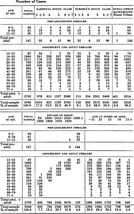
For definitions of educational levels, occupational classes, rural-urban groups, religious groups, etc., see pp. 53-56.
The totals in the occupational and religious classifications amount to more than the totals shown for the entire sample because some individuals had belonged to more than one group in the course of their lives. In tHe rural-urban classification the totals fall short of the total number of cases because some 3 per cent of the females were not identifiable as either rural or urban. For slightly more than 1 per cent of the females in the sample, the data were incomplete and there were individuals who did not fall into the classifications shown above.
Children and dependents derive their occupational classification from that of their parents.
Marital Status . The sample includes many females who had never married, and many who had married (Table 1 ). There is a sizable although still inadequate sample (785 cases) of females who had been widowed, separated, or divorced.
Religious Background . The sample includes females associated with various religious faiths, and variously devoted in their adherence to those faiths (Table 1 ). We have samples of some size (over 500 cases in each) from religiously devout, moderately devout, and inactive Protestant groups, and from moderately devout and inactive Jewish groups. We have 727 histories of Catholic females, including devout, moderately devout, and inactive groups, but obviously need a larger sample of all Catholic groups. We have only 108 histories of devout Jewish females, and that has not been a sufficient sample to allow us to generalize concerning that group at more than a few points in the analyses.
Parental Occupational Class . The sample includes females raised in homes belonging to a variety of occupational classes (Table 2 ). Some 17 per cent of the sample had come from laboring groups, 14 per cent from the homes of skilled laborers, 26 per cent from lower white collar homes, and 47 per cent from upper white collar and professional groups.
Subject’s Occupational Class . The sample includes females belonging to a variety of occupational classes either through their own occupational status or through the status of their husbands (Table 2 ). Out of the total sample, 9 per cent belonged to laboring groups, 3 per cent to the class of skilled workmen, 39 per cent to lower white collar groups, and 59 per cent to upper white collar and professional groups.
Rural-Urban Background . There are females from rural and urban groups (Table 2 ). Some 90 per cent of the total sample was urban. They had lived in a variety of smaller cities and towns, and in some of the larger cities of the United States. Only 7 per cent of the sample (402 cases) had lived on farms for the major portion of the years between the ages of twelve and eighteen. The sample is obviously inadequate for making any final comparisons of rural and urban groups, but such comparisons as we have made show few differences between the two.
Decade of Birth . The sample includes females born in five successive decades. Because they are more abundant in the population, we have secured a larger sample of persons born in more recent decades; but we also have 456 cases of females born before 1900, and 784 cases of females born in the first decade after 1900 (Table 2 ). It has, in consequence, been possible to make comparisons of females born in four successive decades; but in many instances the females born since 1930 had not yet developed their complete patterns of sexual behavior, and their histories therefore cannot be compared with those of the older generations.
Age at Onset of Adolescence . The sample includes females who had turned adolescent at various ages, beginning at some age before eleven and including some who had not turned adolescent until they were fifteen or older (Table 2 ). The age at onset of adolescence, however, has not proved as significant in determining the patterns of sexual behavior among females, as we found it among males.
Geographic Origin . The sample includes females who had lived in various states of the United States (Figures 1 , 2 ). There are still many sections of the country from which we have only limited samples, but it is to be noted that the ten states from which we have our largest series (69 per cent of the total sample) include some 47 per cent of the total population of the United States. These ten states, in order of the size of each sample, are: New York, Pennsylvania, Illinois, Indiana, California, New Jersey, Ohio, Florida, Massachusetts, and Maryland. We need additional cases from the Southeastern quarter of the country, from the Pacific Northwest, and from the high plains and Rocky Mountain areas.
It has been assumed by many persons that we would find geographic differences in patterns of sexual behavior, but we have an impression, as yet unsubstantiated by specific calculations, that there are actually few differences in sex patterns between similar communities in different portions of the United States. The nature of the community in which the individual has lived, whether it be a large metropolitan center, a smaller city, a large or small town, a small farm, or a large ranch in a relatively uninhabited portion of the country, seems to be of greater significance than the geographic location of the area.
Inadequacies of Present Sample . To recapitulate, we may again point out that our present sample is inadequate at many points (Tables 1 , 2 ), and the generalizations reached in the present volume are least likely to be applicable to the following groups:
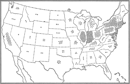
Figure 1. Geographic sources: total female and male sample
Each dot represents 50 individuals who had lived for a minimum of one year in the designated state. The total represents 16,392 cases.
Age groups over 50
Educational level 0–8 (with only grade school education)
Educational level 9–12 (high school), especially among individuals over 40 years of age
Previously married females, now widowed, separated, or divorced
All Catholic groups, especially among older females
Devoutly Jewish groups
Laboring groups (classes 2 and 3), especially among older females
All rural groups
Individuals born before 1900
Groups originating in the Southeastern quarter of the country, from the Pacific Northwest, and from the high plains and Rocky Mountain areas.
We have not been able to work with all of these groups, primarily because only four persons have been available to do the interviewing on this project, and two of us have done the interviewing which accounts for 81 per cent of the total number of histories in our files. We have not been able to find other persons who were available and qualified to meet the demands placed upon an interviewer on this project. In such a special field, an interviewer needs not only considerable professional training, but a personality which enables him to win rapport with persons of diverse social levels ranging from underworld and poorly educated or illiterate groups to socially superior and top professional groups. Moreover, the interviewer must be able to accept a record of any type of sexual activity, whether it is socially acceptable or taboo, or even damaging to the social organization, without passing judgment on the subject who is giving the record, and without wishing to control or redirect his behavior. This ability to accept without attempting to redirect the subject’s behavior is the most difficult quality to find, particularly among clinically trained persons.
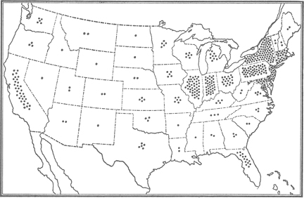
Figure 2. Geographic sources: female sample on which present volume is based
Each dot represents 25 individuals who had lived for a minimum of one year in the designated state. The total represents 5940 cases.
While the necessity for preserving confidence makes it impossible to identify the particular groups from which histories have been obtained in the present study, the following summary will show something of the diversity and limitations of the groups with which we have worked:
Armed Forces
WAC
WAVES
Nurses
Artists
Business office groups
Officers and administrators
Clerks
Technicians
Church congregations
Church organizations
City community groups
Clinical groups, patients and staff
Hospitals
Psychiatric clinics
Psychologic clinics
Mental hospitals
Speech clinics
Sterility clinics
Social service groups
College classes in:
Psychology
Sociology
Biology
Chemistry
Public health
Family living
Horne economics
English
College faculties
College student groups
Sororities
Social clubs
Rooming houses
Rooming houses
Cooperative houses
Religious groups
Court officials
Detention homes
Residents
Staffs
Editorial staffs, magazines
Factory groups
Family groups
Grade school students
Public schools
Private schools
High school students
Public schools
Private schools
Housewives
On farms
In small towns
In cities
Homes for unmarried mothers
Medical organizations
Medical school groups
Mothers’ clubs
Museum staffs
Music schools
Nursery school children
Nurses groups
Orphans’ homes
Parent-teacher groups, in:
Nursery schools
Grade schools
High schools
Public schools
Private schools
Small towns
Cities
Prison staffs
Professional organizations of:
Marriage counselors
Physicians
Administrators of correctional institutions
Salvation Army
Congregations
Children’s clubs
Adult clubs
Staff
Theatre groups
Actors
Managements
Union organizations
Women’s clubs
American Association of University Women
Professional women’s clubs
Women’s service clubs
U.S.O.
Y.W.C.A. groups
An examination of the distribution of the sample shown in Tables 1 and 2 may be more informative than any listing of the groups or of the other characteristics of the persons with whom we have worked. Statistically still more valuable information about the sample may be obtained from an examination of the sample sizes shown in the ultimate breakdowns (the cells) in the various tables in the book.
On the other hand, from an examination of such statistics, one still may not comprehend how many different sorts of persons have been willing to contribute their histories to the present project. In order to emphasize the fact that persons in many walks of life have contributed to the statistics which are summarized and analyzed in the present volume, we submit the following lists showing (1) the occupations of the females in the sample, and (2) the occupations of the husbands of the married females in the sample:
OCCUPATIONS OF FEMALE SUBJECTS
Acrobat
Actress
Advertiser
Airline hostess
Anthropologist
Archeologist
Architect
Art critic
Art director
Art model
Artificial flower maker
Artist
Auditor
Baby-sitter
Bacteriologist
Baker
Barmaid
Beautician
Berry picker
Boardinghouse operator
Bookbinder
Bookkeeper
Burlesque performer
Bus girl
Business executive
Buyer
Cafeteria manager
Camp counselor
Car hop
Cartoonist
Cashier
Checker
Chemist
Cigarette girl
Circus rider
Claim adjuster
Collector
Comptometer operator
Confectioner
Cook
Copy writer
Dancer
Dancing teacher
Dean of girls
Dean of women
Dental assistant
Dentist
Designer
Dice girl
Dietician
Director of foundation
Director, religious educ.
Draftsman
Dramatic critic
Dramatic teacher
Dress designer
Drill press operator
Druggist
Economist
Editor
Electrician
Elevator operator
Employment agent
Expediter
Factory worker
Farmer
Fashion model
Fashion publicist
Foreman
Garment worker
Girl Scout executive
Glass blower
Governess
Gymnasium instructor
Hat check girl
Hospital administrator
Hospital attendant
Hostess
Hotel manager
House mother
Housewife
Illustrator
Inspector
Insurance underwriter
Interior decorator
Interpreter
Interviewer
Inventor
Job analyst
Journalist
Judge
Laboratory technician
Laundress
Lawyer
Lecturer
Librarian
Linotype operator
Lobbyist
Machine operator
Maid
Male impersonator
Manicurist
Manikin maker
Marriage counselor
Master of ceremonies
Matron in orphans’ home
Mechanic
Messenger
Milliner
Minister
Missionary
Movie editor
Movie scout
Museum guide
Music critic
Music teacher
Musician
Night club mgr.
Nurse, practical
Nurse, registered
Nurse’s aide
Occupational therapist
Odd jobs
Office clerk
Office manager
OSS operative
Osteopath
Packer
Paleontologist
Parole officer
Personnel worker
Photographer
Physician
Physiotherapist
Poet
Policewoman
Politician
Potter
Press agent
Presser
Principal, grade school
Principal, high school
Probation officer
Producer (plays)
Professional ballplayer
Proofreader
Proprietor
Prostitute
Psychiatrist
Psychologist
Psychometrist
Public health nurse
Public relations worker
Publicity director
Publisher
Puppeteer
Radio announcer
Real estate agent
Receptionist
Recreation director
Reporter
Research assistant
Research worker
Riveter
Robber
Salesclerk
Sales demonstrator
Sales manager
Sales promoter
Salvation Army officer
Sculptress
Seamstress
Secretary
Shipping clerk
Singer
Social worker
Soda jerker
Speech therapist
Statistician
Steel burner
Stewardess
Student, college
Student, grade school
Student, graduate school
Student, high school
Student, nursery school
Stylist
Supt. of schools
Tavern proprietor
Taxi dancer
Taxi driver
Teacher, college
Teacher, grade school
Teacher, high school
Teacher, kindergarten
Teacher, nursery school
Telegrapher
Telephone operator
Teletype operator
Theatre director
Timekeeper
Traffic manager
Translator
Travel bureau mgr.
Truck driver
Tutor
Typist
Unemployed
Union organizer
Usher
Vocational counselor
WAC
Waitress
WAVE
Weaver
Welder
Window decorator
WPA employee
Writer
X-ray technician
Y.W.C.A. executive
Y.W.C.A. staff
OCCUPATIONS OF HUSBANDS OF FEMALE SUBJECTS
Abortionist
Accountant
Actor
Advertiser
Agricultural agent
Anthropologist
Archeologist
Architect
Army, private to general
Art critic
Art director
Artist
Auto dealer
Aviation pilot
Bacteriologist
Bailiff
Baker
Ballplayer, professional
Banker
Bartender
Beautician
Bellhop
Bookbinder
Bootlegger
Boxer
Boys’ club director
Boy Scout executive
Brewer
Bricklayer
Broker
Buffer
Burglar
Bus boy
Business executive
Business owner (small to large)
Butcher
Buyer
Camp director
Car dealer
Caretaker
Carnival worker
Carpenter
Cartographer
Cartoonist
CCC administrator
Chauffeur
Chef
Chemist
Chiropodist
Chiropractor
City manager
Claims adjustor
Clothier
Coach, athletic
Coast Guard
Collector, financial
College administrator
Comedian
Commercial artist
Composer
Comptroller
Concert manager
Contractor
Copy boy
Counselor
Crane operator
Credit manager
Croupier
Custom’s collector
Cutter, dress
Cutter, metal
Dancer
Delivery boy
Dental technician
Dentist
Designer
Detective
Diamond cutter
Diplomat
Dispatcher
Doorman
Draftsman
Dramatic critic
Dramatic teacher
Druggist
Economist
Editor
Electrician
Electroplater
Engineer, aeronautic
Engineer, chemical
Engineer, civil
Engineer, electrical
Engineer, industrial
Engineer, mechanical
Engineer, radio
Entomologist
Expediter
Explorer
Exporter
Factory manager
Factory worker
Farmer
Filling station attendant
Financier
Fireman, city
Fireman, industrial
Fisherman
Floor sander
Florist
Foreman
Forester
Funeral director
Furrier
Gambler
Garment worker
Geologist
Glass blower
Glazier
Golfer, professional
Grocer
Hairdresser
Handyman
Hat blocker
Horticulturist
Hospital administrator
Hospital attendant
Hotel manager
Hotel staff member
Importer
Insect exterminator
Inspector
Insurance adjuster
Insurance salesman
Interior decorator
Interpreter
Interviewer
Inventor
Investigator
Janitor
Jeweler
Jobber
Journalist
Judge
Laboratory technician
Labor negotiator
Landscape gardener
Lather
Lawyer
Layout artist
Lecturer
Lens grinder
Librarian
Linotype operator
Longshoreman
Lumberjack
Machinist
Mailman
Manufacturer
Market researcher
Mason
Mechanic
Merchant
Messenger
Metal worker
Metallurgist
Meteorologist
Mine superintendent
Miner
Minister
Missionary
Motorman
Movie agent
Movie director
Movie producer
Music critic
Music teacher
Musician
Mycologist
Narcotics inspector
Navy, seaman to commander
Office clerk
Office manager
Oil producer
Optometrist
Orchestra leader
OSS operative
Osteopath
Painter, house
Painter, sign
Park supervisor
Parole officer
Pattern maker
Pawnshop owner
Personnel worker
Photographer
Physical educ. instructor
Physician
Physicist
Physiologist
Piano tuner
Pile driver operator
Pilot trainer
Pimp
Pipe fitter
Plasterer
Plumber
Podiatrist
Poet
Policeman
Polisher
Politician
Porter
Press agent
Press operator
Presser
Principal, grade school
Principal, high school
Printer
Probation officer
Production manager
Promoter
Proofreader
Prosecutor
Prospector
Prostitute
Psychiatrist
Psychologist
Psychometrist
Public opinion research
Publicity man
Publisher
Racketeer
Radar expert
Radio announcer
Radio mechanic
Railroad conductor
Railroad engineer
Railroad fireman
Railroad section hand
Railroad yardmaster
Rancher
Real estate agent
Reporter
Research worker
Riveter
Roofer
Safety engineer
Sailor
Sales clerk
Sales manager
Salesman, city
Salesman, traveling
Salvation Army officer
School superintendent
Sculptor
Sea captain
Sewing machine operator
Sheet metal worker
Shipping clerk
Social worker
Speech therapist
Sprayer
Stationary engineer
Statistician
Steel worker
Steward
Stock boy
Street car conductor
Student
Subway conductor
Swimming instructor
Switchman
Tailor
Tax collector
Tax expert
Taxi driver
Teacher, college
Teacher, grade school
Teacher, high school
Teamster
Telegrapher
Telephone lineman
Telephone operator
Thief
Ticket agent
Tile setter
Timekeeper
Tire changer
Tool and die maker
Traffic manager
Tree surgeon
Truck driver
Tutor
Unemployed
Union organizer
Upholsterer
Veterinarian
Vocational adviser
Waiter
Watch repairman
Watchman
Weaver
Welder
Window designer
Wire tester
WPA employee
Writer
Y.M.C.A. executive
Y.M.C.A. staff
Although we have so far taken 7789 histories of females, the statistical calculations in the present volume have been confined, as we have already noted, to the 5940 cases of white, non-prison females whose histories we had acquired prior to January 1, 1950. By closing the sample on that date, it has been possible to hold the total number of cases (the N) more or less constant in the tabulations and calculations throughout the book; but the totals fall short of 5940 in most of the calculations for the following reasons:
1. Question Inapplicable . Very often a particular question does not apply to the entire sample. This is the chief reason for the occurrence of N’s which are smaller than the N of the total sample. For instance, questions concerning marital coitus do not apply to single females; questions concerning menstruation do not apply to pre-adolescent females.
2. Uncertain Behavior . Sometimes there are uncertainties as to the nature of the behavior in which a subject has engaged. It may, for instance, be impossible to determine whether the incidental touching of genitalia should, in a given case, be considered masturbation or nonsexual activity. Sometimes it is difficult to determine whether there was erotic arousal in connection with the activity. There is usually no question whether the subject did or did not experience orgasm from masturbation or some other source, and, in consequence, the number of cases (the total N) on which the incidences of experience may be calculated is sometimes different from the number of cases on which we may calculate the incidences of experience to orgasm. Therefore the samples that are used for the two sorts of calculations are sometimes different, and for that reason there are a few places in the present volume where the active incidences of orgasm are a bit higher than the accumulative incidences of experience at the same age.
3. Question Not Asked . The N’s are sometimes lower than 5940, and sometimes markedly lower than that number, when a particular question was not asked of all of the subjects in the study. From a very early point in the history of the research, a high proportion of all the questions have been uniformly asked on each interview, but something over 20 per cent of the present questions were not asked in the first year or two. Consequently the number of cases available for analyses on such items is lower than the number of cases in the total sample. Some additional questions have been introduced in more recent years, e.g. , questions concerning extra-marital petting, questions concerning the female’s erotic response upon seeing male genitalia, and questions concerning the acceptance of homosexual friends. A few of the questions which were asked in the earlier part of the research were dropped from the interviews in the last few years because the answers were so uniform that there seemed no point in obtaining additional information.
4. Interviewer’s Failure . The N’s in some instances are lower than the total N because the interviewer failed to obtain information on the particular point. These failures have been relatively few because the standard form in which the interview is coded provides a simple check by which the interviewer at the end of an interview can make sure that all the questions have been answered. Interviewer failures have been most frequent in those periods in which new questions were being added, and when the interviewer had not yet become accustomed to exploring in those areas.
5. Refusal to Reply . This is responsible for only minor reductions in the total N’s, and then on only a very few items. Unlike the experience of those engaged in public opinion and some other surveys, we find no difficulty in getting our subjects to answer all of the questions in an interview. In the course of the fourteen years, there have not been more than a half dozen subjects who have refused to complete the records after they had once agreed to be interviewed.
6. Insufficient Information . The interviewer’s failure to secure sufficient or exactly pertinent information on certain items may account for some of the instances in which the available N’s are lower than the total N. This sort of failure does the most damage when the final calculations are based upon some coordination of several answers. Then a failure to obtain data on any one of the points may make it impossible to use any of the answers in the group. For instance, the failure to secure a record of the frequencies of orgasm in pre-marital coitus would make it impossible to use the given history in correlating the pre-marital with the subsequent marital experience.
In our previous volume, nearly all of the statistical calculations were based upon the male’s experience in sexual activity which had led to orgasm. Although the male is frequently aroused without completing his response, he rarely engages in such activities as masturbation or coitus without proceeding to the point of orgasm. On the other hand, a considerable portion of the female’s sexual activity does not result in orgasm. In consequence, statistical calculations throughout the present volume have shown, wherever the data were available, the incidences and frequencies both of the female’s sexual experience and of her experience in orgasm.
It is usually possible to secure data on the incidences of sexual experience that did not lead to orgasm, but it is often impossible to secure frequency data on such experience, because of the difficulty of distinguishing between non-erotic social activities—a simple kiss, for instance—and similar activities which do bring erotic arousal. On the other hand, orgasm is a distinct and specific phenomenon which is usually as identifiable in the female as in the male. It has served, therefore, as a concrete unit for determining both incidences and frequencies. The use of such a unit is justified by the fact that all orgasms, whether derived from masturbation, petting, marital coitus, or any other source, may provide a physiologic release from sexual arousal; but since there may be differences in the social significance of orgasms obtained from one or another type of activity, there has been some objection to the use of that phenomenon as a unit of measurement. The matter is further discussed in Chapter 13 (pp. 510–511). There seems, however, no better unit for measuring the incidences and frequencies of sexual activity. As we have already noted, a considerable portion of the present volume is concerned with reporting other aspects of sexual behavior which are not so readily quantified for statistical analyses.
The following definitions are designed to give the non-statistical reader an acquaintance with the meanings of some standard statistical terms. For the technically trained reader, these definitions will show the way in which the terms have been applied in the present volume.
Accumulative Incidence . An accumulative incidence curve shows, in terms of percentages, the number of persons who have ever engaged in the given type of activity by a given age. The calculations are, of course, based on the experience which the reporting subjects had had before contributing histories to the present study; but by securing information on the age at which each subject had first had experience, it is possible to determine the percentage of the total sample who had had experience at each age up to the time of interview. But an accumulative incidence curve may also be useful in indicating what percentages of any group might be expected to have experience if they were to live into the older age groups. A fuller explanation of the techniques involved in calculating these curves is given in our volume on the male (1948:114–119).
Most of the incidence data presented in research studies record the number of persons who are having experience in a given period of time, e.g. , the current incidences of venereal disease, or the current incidences of marriage in the U. S. population. The accumulative incidences, on the other hand, show how many persons have ever had experience by a given age. This answers a type of question that is very frequently asked. One may want to know how many persons ever masturbate, how many persons ever have coitus before marriage, how many persons ever have homosexual experience.
A subject’s ability to report whether he has ever engaged in a given type of activity is not as liable to errors of memory and of judgment as his ability to recall frequencies of activity and to estimate the average frequencies of his activity (see also pp. 68–73). A subject’s willingness to admit experience, however, may be affected by society’s attitudes toward particular types of sexual activity—toward pre-marital coitus, extra-marital coitus, mouth-genital contacts, and homosexual contacts, for instance—; and in regard to such items, subjects may occasionally deny their experience. On the other hand, it is more difficult for a subject to exaggerate because of the difficulty in answering subsequent questions concerning the details of the professed experience. The accumulative incidence data are, therefore, probably a minimum record rather than an exaggeration of the experience actually had by the subjects in the study.
Active Incidence . As used in the present study, the active incidences represent, in terms of percentages, the number of persons who have engaged in each type of sexual activity in a particular period of their lives. In our previous and present volumes, these have been standardly expressed as five-year periods, covering in most instances the years between adolescence and fifteen, sixteen and twenty, twenty-one and twenty-five, etc. See our volume on the male (1948:76–77) for a further discussion.
The active incidences for the various age groups provide highly significant data in any sex study, because the number of persons involved in a given type of activity depends upon age more than upon most other factors. However, it should be recognized that any individual who has had a single experience within the five-year period raises the percentage shown in an active incidence. In most instances the active incidences would have been lower if they had been calculated for one-year instead of five-year periods. A better comprehension of the extent of any type of sexual activity may be had if one considers the active incidences in conjunction with the average frequencies among those who are having any experience (the active median frequencies).
Frequency of Activity . The frequency of each subject’s activity is recorded as an average frequency for each of the five-year periods specified above. Throughout our previous and present volumes, frequencies have been expressed as average frequencies per week in each of those periods. The weeks or years in any five-year period which were without sexual activity have been averaged with the weeks or years in which there was activity, and in that way periods of inactivity have lowered the average rates in such a five-year period. Unless the data are specifically designated as applying to pre-adolescence, all of the frequency calculations in the present volume have been based upon activities which occurred after the onset of adolescence. In consequence, the first age period extends from adolescence to fifteen, and in that case the average frequencies are based on the number of adolescent years and are not reduced by being averaged with the preadolescent years. If the last age period—the one in which the subject contributes his or her history, or changes his marital status—is less than a full five-year period, it has been treated in the same fashion as the first adolescent period. No frequency calculations have been made for persons who belonged to a given age, adolescent, or marriage period for less than six months.
Because of the difficulties which most persons have in estimating average frequencies for experience which may have been sporadic or irregular in its occurrence, frequency data are subject to much greater error than incidence data. This explains why there have been few attempts in previous studies to determine the frequencies of sexual behavior. But even though considerable allowance must be made for errors in the frequency data, they show what appear to be significant correlations with age, the decade of birth, the religious associations, and still other social factors in the backgrounds of the females in the sample.
Frequency Classes . In all calculations in the present volume, individuals have been grouped in frequency classes which have been named, throughout both our previous and present volumes, for their upper limits. Since it is current practice in most statistical publication to name frequency classes for their lower limits, attention should be drawn to our different practice. The ranges and the mean values of the frequency classes as we have defined them in our preceding and present volumes, are as follows:
| CLASS | RANGE | MEAN VALUE |
|---|---|---|
| 0 | 0 | 0 |
| 0.09 | 0.01- 0.09 | 0.05 |
| 0.5 | 0.1 - 0.5 | 0.3 |
| 1.0 | 0.6 - 1.0 | 0.8 |
| 1.5 | 1.1 - 1.5 | 1.3 |
| 2.0 | 1.6 - 2.0 | 1.8 |
| etc. | ||
| 10.0 | 9.6 -10.0 | 9.8 |
| 11.0 | 10.1 -11.0 | 10.5 |
| 12.0 | 11.1 -12.0 | 11.5 |
| etc. | ||
| 28.0 | 27.1 -28.0 | 27.5 |
| 29.0+ | 28.1 and higher | 28.5 |
Since most persons report frequencies in terms of whole integers, and since we have used the upper limits of each class to designate the frequency classes into which such reported data are placed, our calculations of both median and mean frequencies have, in actuality, been more conservative than they would have been if we had used the lower limits to designate each class. An individual who reported an average frequency of a given type of sexual activity at 2.0 per week would go, in our calculations, into a class which had a mean value of 1.8 per week. If the lower limits had been used to designate each class, that same individual would have gone into a group which had a mean frequency value of 2.2 per week. However, the differences in the averages obtained by these two methods of calculation are slight and usually immaterial in terms of the quantities being measured.
Median Frequency . When the individuals in any group are arranged in order according to the frequencies of their sexual experience, the individual who stands midway in the group, the median individual, may be located by the formula

Throughout such statistical formulae, the symbol N or n stands for the number of individuals in the group. While the median is an average which is not often calculated by people in their everyday affairs, it is a useful statistic because it is unaffected by the frequencies of activity of the extreme individuals in any sample. The mean, which is the sort of average that most persons ordinarily calculate, is affected by extreme individuals (p. 50). In consequence, median frequencies are the statistics which we have more often used in the present volume.
Active Median Frequency . In any group and especially in any group of females, there may be some individuals who are not having any sexual activity of the sort with which the calculation is concerned. That portion of the total sample which is actually having experience or reaching orgasm has been identified in the present study as the active sample . The median individual of this active sample has a frequency of experience or orgasm which we have identified throughout this volume as the active median frequency .
Total Median Frequency . The entire sample in any group, including both those individuals who are not having experience of the sort under consideration and those who are involved in that particular type of sexual activity, constitutes the total sample as we have used the term in the present study. The median individual in such a total sample has a frequency of activity which we have identified as the total median frequency .
Where less than half of the individuals in a sample are involved in a given type of activity—where, for instance, less than half of the individuals in a given group are petting to the point of orgasm—the median individual is, of course, not having any activity at all. In consequence, the median frequency for such a group is zero. Since the active incidences of many types of sexual activity among females are frequently less than 50 per cent, it has not been possible to calculate total median frequencies on more than a few of the types of sexual activity discussed in the present volume. They have been calculated chiefly for marital coitus and for the total sexual outlet, because more than 50 per cent of the females are actively involved in those activities in most of the age groups.
Mean Frequency . A mean frequency may be determined by totaling the measurements (in the present study, the total number of experiences or total number of orgasms) in each group, divided by the number of individuals in the group. The process is summarized in the formula:

The mean is the sort of average which is most commonly employed by most persons in their everyday affairs. If one wants to find the average price which has been paid for a number of articles, this is done by totaling the individual prices and dividing by the number of objects bought. Such an average is the mean of the various prices which were paid. Conversely, the total amount of money spent may be calculated by multiplying the mean price by the number of objects which were bought. In the same fashion the total number of orgasms experienced in any group may be determined by multiplying the mean frequencies of orgasm by the total number of persons in each group. The mean, therefore, serves a function which is not served by the median.
On the other hand, means often give a distorted picture because their values may be considerably raised by a few high-rating individuals in the group. Since there is usually a tremendous range of variation in the frequencies of sexual activity or of orgasm in any group of females, the mean frequencies are uniformly higher than the median frequencies of sexual activity (e.g. , see Tables 23 , 43 , 76 , 114 ). Since the range of individual variation is more extreme among females than it is among males, mean frequencies calculated for females are even less adequate as measures of sexual activity than they are for males. Consequently mean frequencies have been used in the present volume only when we wished to calculate the total number of experiences, or the total number of orgasms occurring in a whole group.
Active Mean Frequency . The mean frequencies for the females in an active sample—those females who were having any experience, or experience to the point of orgasm—have been designated as the active mean frequencies .
Total Mean Frequency . The mean frequencies of the females in any total sample, including those who were not having experience or orgasm as well as those who were having such experience or orgasm, represent the total mean frequencies, as they are designated in the present volume.
Standard Error . What is known as the standard error or the standard deviation of the mean, the standard error of the mean, or the sigma of the mean, is a quantity which, when added to or subtracted from the mean, shows the limits within which the calculated mean might be expected to differ from the mean of the entire population approximately two-thirds of the time. In the present volume, the standard deviation of the mean has been calculated by using the formula
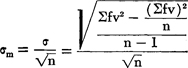
For the general reader it may be pointed out that the standard deviation is appended to the mean in the following form:

When the data involved comparisons of simple yes and no answers, as in Tables 3 –5 , the formula used for calculating the standard error was
Significant Differences . Whether the differences between the calculations made for two or more groups—e.g. , the differences in the frequencies of orgasm calculated for two groups of different ages—are meaningful, or whether they fall within the range of variability that might be expected within either one of the groups, is a matter which may be tested by various statistical techniques. Within certain limits, it may thus be shown that the differences are or are not statistically significant. However, because most sexual data cannot be reported with the sort of precision which is obtainable in making physical measurements, and because the variations in sexual data almost never show normal frequency distributions, it has seemed undesirable to calculate the statistical significances of the differences in our data by methods which are often used for other sorts of data.
Whether a given difference is significant may, however, often be recognized without statistical calculation. This may be possible: (1) When the differences are of some magnitude, relative to the standard errors of the quantities being measured. (2) When the differences represent reasonably measurable quantities (e.g. , frequencies of one orgasm in a matter of a few weeks or a month, and not merely one orgasm in a year or two, which is such a small quantity that few persons could recall and report it with any precision). (3) When the variation in the one group lies entirely outside the range of the variation in the other group. (4) When the differences between the various groups which are in a series lie within a trend, i.e. , accumulate in a given direction between the extreme groups in the series. (5) When the differences between the contrasting groups in any pair, or the extreme groups in any series, lie consistently in the same direction, e.g. , for the different age groups, educational levels, decades of birth, levels of religious devotion, etc. For instance, when the incidences or frequencies of a given type of sexual activity are lower in all or essentially all of the devoutly religious groups, and higher in all the religiously inactive groups, whether Protestant, Catholic, or Jewish, the differences may be considered of some significance.
We have tried not to suggest that any of the differences shown between the groups in the present study are significant unless such a conclusion seemed warranted by this sort of direct inspection of the data.
Unfortunately the term significant has an older, non-statistical use which applies to situations that are meaningful, important , or in some fashion indicative of something. It has not been possible to avoid that use of the word in writing of matters that are so often significant to the individual, or significant to the social organization of which the individual is a part. Wherever this general use of the term might be confused with the more technical use, we have used the phrase statistical significance to distinguish the technical meaning of the term.
Percentage of Total Outlet . In the present volume we have systematically calculated what proportion of the orgasms experienced by each group had been derived from each type of sexual activity. Thus, in a given age group of white females of a particular educational, religious, or other background, we have calculated what proportion of the total number of orgasms occurring in the group had been derived from masturbation, from nocturnal dreams to orgasm, from pre-marital coitus, etc. Obviously, the sums of the percentages shown for the several types of sexual activity must constitute one hundred per cent of the total outlet (the total number of orgasms) of the group.
We have not calculated the percentage of the total outlet which was derived by each individual from each type of sexual activity, and then calculated averages based on those individual data, as we did at a few points in our volume on the male.
Coefficient of Correlation . In attempting to show the extent to which two phenomena may be correlated in their occurrence, it has been customary in certain fields to express such correlations by coefficients which are calculated by standard statistical formulae. In our volume on the male, we restricted the use of such coefficients to the comparisons of original histories and retakes, and to the comparisons of data contributed by paired spouses. However, our direct comparisons of the calculated incidences and frequencies seem more meaningful for the sorts of data we have in this study, and we have not used correlation coefficients at any point in the present volume.
Age . For each type of activity, the ages at first experience and the ages during which there was subsequent experience have been standardly recorded and calculated for each year in each history. However, as a matter of economy, and as an aid to the comprehension of the total picture, the accumulative incidence data have been published only for each fifth year, except when there were unusual or marked developments in the intervening years. In the latter event, we have published the record for those years.
Marital Status . In most calculations in this volume, sexual activities have been classified as occurring among single, married, or previously married females. Individuals were identified as single up to the time they were first married. They were identified as married if they were living with their spouses either in formally consummated legal marriages, or in common-law relationships which had lasted for at least a year. They were classified as previously married if they were no longer living with a spouse because they were widowed, divorced, or permanently separated. These definitions are more or less in accord with those used in the U. S. Census for 1950, except that common-law relationships have been more frequently accepted as marriages in our data, and we have considered any permanent separation of spouses the equivalent of a divorce.
Educational Level . On the basis of the educational levels which they had attained before completing their schooling, the females in the sample have been classified in four categories, as follows:
| 0– 8: | those who had never gone beyond grade school |
| 9–12: | those who had gone into high school, but never beyond |
| 13–16: | those who had gone into college, but had not had more than four years of college |
| 17+: | those who had gone beyond college into post-graduate or professional training |
It was obviously impossible to determine the educational level that would ultimately be attained by subjects who were still in grade school or high school at the time they contributed their histories, and they were consequently unavailable for any calculation that involved an educational breakdown. Persons still in college were classified among those having 13 to 16 years of schooling, and this may have involved a small error because a portion of them would ultimately go on into graduate work.
Upon calculation, we find that educational backgrounds do not seem to have been correlated with the patterns of sexual behavior among females as they were among the males covered by our previous volume. Consequently in the present volume we have published direct correlations with most of the other factors, such as decade of birth and religious background, without showing the preliminary classifications which we have made on the basis of the educational levels.
Occupational Class of Parental Home . Since the female’s social status after marriage depends on the occupational class of her husband as well as upon her own social background, it has not proved feasible to make correlations, as we did in the case of the male, with the female’s own occupational rating. However, in the present volume we have correlated the incidences and frequencies of her sexual activities with the occupational class of the parental home in which she was raised. If the parental home had changed its social status during the time that the female lived in it, she was given a rating in each of the occupational classes. The occupational classes have been defined as they were defined in the case of the male:
(1) Underworld: deriving a significant portion of the income from illicit activities
(2) Unskilled laborers: persons employed by the hour for labor which does not require special training
(3) Semi-skilled laborers: persons employed by the hour or on other temporary bases for tasks involving some minimum of training
(4) Skilled laborers: persons involved in manual activities which require training and experience
(5) Lower white collar groups: persons involved in small businesses, or in clerical or similar work which is not primarily manual and which depends upon some educational background
(6) Upper white collar groups: persons in more responsible, administrative white collar positions
(7) Professional groups: persons holding positions that depend upon professional training that is beyond the college level
(8) Persons holding important executive offices, or holding high social rank because of their financial status or hereditary family position
For further definitions and a discussion of these classes, see our volume on the male (1948:78–79).
Decade of Birth . Correlations with the decade of birth have been based, in the present volume, primarily on the four following groups:
Born before 1900
Born between 1900 and 1909
Born between 1910 and 1919
Born between 1920 and 1929
The decade of birth has proved to be one of the most significant social items correlating with the patterns of sexual behavior among American females. In many instances the youngest females in the sample, born since 1929, had not developed their patterns of sexual behavior far enough or been married long enough to warrant their inclusion in any of the comparisons of generations.
Age at Onset of Adolescence . Correlations have been made with the age at which the female showed the first adolescent developments (pp. 122–125). The classifications have been as follows:
Before and at 11 years of age
At 12 years of age
At 13 years of age
At 14 years of age
At 15 years of age or later
Rural-Urban Background . The subjects in the present study have been classified as having rural backgrounds if they lived on an operating farm for an appreciable portion of the time between the ages of twelve and eighteen. This is the pre-adolescent and adolescent period which is of maximum importance in the shaping of sexual patterns. The more extensive classification of rural and urban backgrounds given in our volume on the male (1948:79) would have provided a more satisfactory basis for correlations, but unfortunately we do not yet have enough histories of rural females to allow us to make such an intensive study.
Religious Background . Subjects in the present study have been classified as Protestant, Catholic, or Jewish, or as belonging to some other group. In these other groups (1.3 per cent of the total sample) the number of histories is too small to allow analyses. In each of the three religious groups, the subject has been classified as devout, moderately religious, or religiously inactive, in accordance with the following definitions:
(1) DEVOUT : if the subject is regularly attending church, and/or actively participating in church activities. If Catholic, frequent attendance at confession is a criterion; if Jewish, frequent attendance in the synagogue, or the observation of a significant portion of the Orthodox custom.
(2) MODERATELY RELIGIOUS : if the subject attends church or engages in church activities with fair frequency, or attends confession in the Catholic church, or follows the Orthodox custom to some degree which, however, is less than that of strictly devout groups.
(3) RELIGIOUSLY INACTIVE : if the subject only infrequently, or rarely, or never attends church or engages in church activities, or infrequently or never goes to confession, or observes few if any of the Orthodox Jewish customs. Such persons may still, however, be related to one or another of the religious groups through their parents, through their own earlier training, or through their own current thinking. There have been exceedingly few persons in the study who are as completely irreligious or agnostic as they often insist.
It has been possible to correlate the sexual data on these histories with the current religious status of each subject, but it has not yet been possible to make correlations with their earlier religious connections. The earlier connections may have been the more significant in affecting the subsequent patterns of sexual behavior, but we will need a more extensive series than we yet have before we can undertake further analyses.
There are obviously still other factors which affect patterns of sexual behavior and which deserve investigation. For instance, the age at which the female marries may markedly affect the nature and the extent of her pre-marital experience, particularly in pre-marital petting and in pre-marital coitus. Consequently we have made correlations with the age of marriage at certain points in the present volume. On the other hand, some of the other correlations that may ultimately deserve investigation, such as the correlation with the geographic location and the type of community in which the subject was raised, cannot be made until we have secured additional data.
U. S. Estimates . In our volume on the male we attempted to estimate the incidences and frequencies of the various types of sexual activity in the total U. S. population, by weighting and combining the data for the age groups, the single, married, and previously married groups, the educational groups, and the rural and urban groups in the sample, in accordance with the incidences of those groups in the United States Census of 1940. Such a correction seemed desirable in order to prevent the general reader from making his own extensions of the data without any correction for census distributions.
The research scientist may choose between two possible procedures in presenting his data. He may present the material as a description of his findings on the particular individuals with which he worked, and make no suggestion concerning any possible extension of his generalizations to any larger group; or he may attempt, by some statistical or other technique, to discuss the applicability of his findings to some group larger than the one with which he actually worked. If he follows the first procedure, he imposes upon the reader the task of deciding how far to extend the specific findings, and the reader is usually more poorly equipped than the scientist to decide that. For instance, if we had not attempted a U. S. correction in the male volume, our data on the incidences and frequencies of masturbation, because of the larger representation of college males in the sample, would have given an exaggerated picture to any reader who took them to be typical of American males in general; and our data on the incidences and frequencies of pre-marital coitus would have represented a gross understatement for the total population because of the lesser representation of grade school and high school groups in the sample.
We have not, however, undertaken to do U. S. corrections in the present volume, because our sample of females is even more inadequate than our sample of males in representing lower educational levels, rural groups, and some of the other segments of the population (p. 36). The generalizations made throughout the present volume have, therefore, been restricted to the particular samples that we have had available. Major changes might have been introduced into the generalizations if we had had a larger sample of females who had never gone beyond grade school, but we cannot suggest what those changes might have been. Meanwhile, the samples of high school, college, and post-graduate groups are of some size, and the generalizations drawn for the sample may not be too far from the actuality for those segments of the American population.
1 For general discussions of sampling methods, see such statistical texts and articles as the following: U. S. Bureau of the Census 1947. Yates 1949. Deming 1950. Lorie and Roberts 1951. Cochran 1953.
2 Probability sampling has been used, for instance, in the following, among other surveys: Federal Reserve Bulletin 1946–1953 (annual surveys of consumer finances). Dinerman 1949 (election predictions Elmira, N. Y.). Public Opinion and Sociological Research Division, SCAP, 1950:452–453 (attitudes toward foreign countries and questions on international affairs, Japan). Deming 1950: 372–398 (population study for Greek government). Washington Public Opinion Laboratory 1950 (attitudes on marriage and divorce, state of Washington). Belknap and Campbell1951 (preferred presidential candidate, religion, income, attitudes on sending troops to Korea, national sample). Crespi 1951 (German view of U. S. reorientation program). Crossley and Fink 1951 (satisfaction with living in Denver). Maccoby 1951 (television, its impact on school children, in Cambridge, Mass.). Radvanyi 1951 (economic and cultural characteristics of rural population of Santiago Valley, Nayarit, Mexico). Hemphill 1952 (home injuries in Washtenaw Co., Mich.). Horvitz 1952 (Pittsburgh morbidity survey). See also surveys by U. S. Bureau of Labor Statistics published in various Department of Labor bulletins, for example Nos. 956 (1949) on family income, and 1065 (1952) on expenditures and savings. Examples of other probability surveys may be found in the Journal of the American Statistical Association and in the journal, Population Studies.
3 Reports on the rates of non-response in various studies may be found in: Dinerman 1949 (18 per cent failure to complete interviews). Heneman and Paterson 1949 (discussion of interviewer effectiveness vs. refusals). Crossley and Fink 1951 (14 per cent non-completion of interviews). U.S. Bureau of Labor Statistics (Bulletin 1065) 1952 (surveys, in a difficult problem, for 10 cities with non-completion rates from 2 per cent to 34 per cent; over-all non-completion 26 per cent).
