Chapter 12
The Solution of Linear Fractional Differential Equations Based on the Fractional Trigonometry
This chapter develops methods for the solution of linear constant-coefficient fractional differential equations of any commensurate order. Classes of fractional differential equations with unrepeated roots, repeated real roots, and repeated complex conjugate roots are considered. The solutions for the case of unrepeated roots are implemented using simplified Laplace transforms based on the fractional meta-trigonometric functions and the R-function as developed in Chapter 3. The solution of fractional differential equations with repeated roots, additionally require application of the G- and H-functions, which were studied in Chapter 3.
12.1 Fractional Differential Equations
Driven by our need to understand and codify the physical world, the major objective of the fractional calculus is the formation and solution of fractional integral and, more importantly, fractional differential equations. There has been considerable effort toward the solution of fractional differential equations going back to the work of Heavyside [51], Davis [26], and others.
More recently, the works of Oldham and Spanier [104], Miller and Ross [95], Samko et al. [114], West et al. [121], and Oustaloup [105] have contributed to the development of the fractional calculus as well as to the solution of fractional differential equations. Furthermore, Podlubny [109] has written an important book dedicated to the solution of fractional differential equations.
These works and others present various dedicated approaches to the solution of specialized and general fractional differential equations. The development of the fractional trigonometries of Chapters 5–9 may be applied to the solution of fractional differential equations. In particular, the fractional meta-trigonometric functions developed in Chapter 9 applies toward more general classes of equations.
Application of the fractional trigonometric functions to the solutions of linear fractional differential equations has been treated by Lorenzo, Hartley, and Malti [87, 88] and is the basis of this chapter.
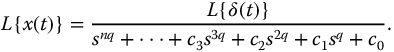
Fractional differential equations of the form

are known as commensurate order due to the constraining relationship of the order of the derivatives. Our goal is to find the solution of such linear fractional differential equations of any commensurate order when the coefficients ci are constants. The related Laplace transform for equation (12.1) with zero initial conditions is the transfer function

The method for solution of equation (12.1) is similar to that required for ordinary linear differential equations (i.e., equation (12.1) with q = 1), with constant coefficients. The procedure for ordinary linear differential equations with constant coefficients is to factor the related transfer function into sums of first- and second-order subsystems; that is, into sums of the forms ks/(s + a) or k/(s + a) for the first-order subsystem and k/(s2 + bs + c), ks/(s2 + bs + c) or ks2/(s2 + bs + c) for the second-order subsystems. Inverse transforming the subsystems yields solutions that are sums of time functions, which are combinations of real exponential functions and the classical sine and cosine functions.
The approach developed here for the solution for fractional differential equations of the form of equation (12.1) is similar to that used for ordinary linear differential equations. That is, the transfer function (12.2) is decomposed (factored) into the sum of subsystems elements with denominators of the qth and 2qth order. These subsystems, known as elementary transfer functions of the first and second kinds, are of the respective forms

It is important to note that Podlubny [109] has solved fractional differential equations that generalize the form of equation (12.1) using infinite summations of generalized Mittag-Leffler functions. The solutions to be developed here will be in terms of the simpler fractional trigonometric functions.
Linear fractional differential equations of the form

have been referred to as the fundamental fractional differential equation, as discussed in Chapter 2. The solutions of this equation may be expressed in terms of R-functions with real arguments. The more general form

is shown to have solutions that can be represented as fractional trigonometric functions. As we have seen, fractional trigonometric functions are real functions based on the R-function with complex arguments, namely

The fractional trigonometries (of Chapters 5–9) define a wide variety of oscillatory and non-oscillatory fractional functions that are solutions or components of solutions to such linear fractional differential equations.
In equation (12.1), we use the notation  to indicate the initialized fractional derivative of the qth order. Then,
  , where
  is the uninitialized derivative and
  is the time-varying initialization function (see, e.g., [68, 71, 78]). The effect of the initialization terms is to add time-varying terms to the right-hand side of equation (12.1). These terms contribute the initialization response of the solution. Inclusion of the initialization terms will distract from the objectives of this chapter and for simplicity of presentation, only the forced response is considered. Therefore, it is our goal to solve uninitialized fractional differential equations of the form

A secondary goal is to create specialized versions of the Laplace transforms of the fractional meta-trigonometric functions to allow easy application to the solutions of equation (12.7). The following sections discuss the solutions for the elementary functions of the first and second types.
12.2 Fundamental Fractional Differential Equations of the First Kind
Elementary transfer functions of the first kind (equation (12.4) derive from the fundamental fractional differential equation

which was introduced in Chapter 2. Solutions to this equation are based on the F-function detailed in Chapter 2. The more general case

was considered in Chapter 3. Under quiescent initial conditions, the Laplace transform was shown to be

When  , a unit impulse, the solution to equation (12.8) may be written in terms of the R-function. Its Laplace transform was shown to be

Then,

provides the solution to equation (12.9). Less conveniently, some of the Mittag-Leffler-based functions of Table 3.1 may be used in some instances for solution to equation (12.9). When  , the solution may usually be obtained by application of the convolution theorem to equation (12.10).
Differential equations of this type may also be solved using the following transform pairs, for c0 > 0,


and for c0 < 0


Furthermore, in some cases, it may be useful to specialize the fractional meta-trigonometric functions (Table 9.2) for the solution of equation (12.9).
12.3 Fundamental Fractional Differential Equations of the Second Kind
Elementary transfer functions of the second kind, first studied by Malti et al. [91], relate to fractional differential equations of the form

with c0 and c1 real. The Laplace transform associated with this equation is given by

In general, fractional differential equations of the second kind and their transforms are needed for the solution of higher-order fractional differential equations with complex roots in the characteristic equation.
The denominator of equation (12.17) is quadratic in  and its behavior is dependent on the discriminant,
  , that is, for
  , the roots are complex conjugates, the case of interest for fractional differential equations of the second kind. The fractional trigonometric functions of Chapters 6–8 provide solutions to particular cases of equation (12.16). The Laplace transforms for the meta-trigonometric functions (Table 9.2) more broadly apply. Solutions related to equation (12.16) are shown using either the fractional cosine or fractional sine functions in the following sections.
12.4 Preliminaries – Laplace Transforms
The Laplace transforms developed in Chapter 9 are simplified for more direct application to the solution of fractional differential equations. In particular, simplified Laplace transform pairs based on those previously determined for the fractional trigonometric functions are developed for the solution of equation (12.16). This section is adapted from Lorenzo et al. [87, 88]. Note that the mathematical results in Ref. [87] have systemic errors and should not be used. Errors in previous versions have been corrected here. Proceeding with permission of ASME and the Royal Society:
12.4.1 Fractional Cosine Function
The Laplace transform of the fractional cosine function is given as

where  . To reduce the number of parameters in this equation and in other equations to follow, we consider only the principal functions. That is, we take k = 0; thus,

where  . This Laplace transform is now specialized for application to equation (12.17). For
  , a unit impulse, we take
  , and let
  . From these conditions, the following requirements are determined:

For simplicity of results, take m = 1

Now, we also require  . When
  , the roots are complex conjugates. Then,

But we must also have that

Solving for 

Now, we can write

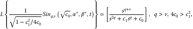
These results give the useful transform

where  are given by equations (12.20) (12.18), and (12.19), respectively, and the star superscripts are introduced to indicate that the values apply only to the formulation of this section. Thus, the forced response solution for equation (12.16), with
  a unit impulse, is given by

When  is not the unit impulse, the convolution theorem may be applied to evaluate the solution.
Because the following transform pairs are derived in a similar manner, and apply under different constraint conditions, only the results are given.
12.4.2 Fractional Sine Function
The principal fractional sine function may also be the basis of a simplified Laplace transform. We start from the transform pair

where  and
and  . The
. The  -based transform is given by

The star superscripts indicate that the values apply only to this formulation, and  is given by

12.4.3 Higher-Order Numerator Dynamics
12.4.3.1 Fractional Cosine Function
We also require Laplace transforms of the form

This form is not covered by either equation (12.21) or (12.24) because of the limiting constraints on those equations. The Laplace transform of the fractional cosine function is

where  . The result for the fractional cosine function is

where  are given by

12.4.3.2 Fractional Sine Function
A Laplace transform with a higher order of the numerator term may be based on the fractional sine function [88]

where  follows. The transform pair is given by
where  and
and  are
are

12.4.4 Parity Functions – The Flutter Function
The parity functions may also be used to solve the fundamental fractional differential equation of the second kind. Here, only the Flutter function is considered, and its Laplace transform is given as

where  . Letting q = w/2, we have

where  . Now, let
  ,
, 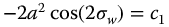 ,
,  , and
, and  .
.
Then,  and from
 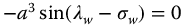 , we have

From  ,
,

Using  , we have

A useful transform pair based on the fractional meta-trigonometric parity function (equation (12.32) is given as

where  are given by equations (12.33) and (12.34), respectively.
12.4.5 Additional Transform Pairs
There is considerable interest in elementary transfer functions of the second kind, defined by Malti et al. [91]. The Laplace transform of interest is

where  is a fractional generalization of natural frequency and
  has been named the pseudo-damping factor. Here, we consider the related form

Both the fractional sine and cosine functions may be used to achieve such transforms. Here, the sine function (equation (12.23) is considered with  and
and  . Thus, we have the Laplace transform as

where  is given by

The fractional cosine function may also be used to obtain transform pairs related to equation (12.4.5.2). For this case, we have the result

where  , and
, and

Note that in the previous simplified transform pairs the constraint  (or
(or  ) was needed to assure complex conjugates roots and the applicability of the fractional trigonometric functions. In the case where
  , the roots are real. In this case, the factorization process should yield the real roots, and the resulting inverse transforms takes the form of R-functions or fractional hyperbolic functions, that is, equations (12.14) or (12.15). The latter case, of course, results in unstable behavior. Stability behavior for the elementary transfer functions is discussed in Section 2.5 and in Sections 13.6–13.8.
12.5 Fractional Differential Equations of Higher Order: Unrepeated Roots
The Laplace transforms presented in the previous sections together with the R-function may now be used to solve any linear constant-coefficient fractional differential equation of commensurate order, that is, equations of the form

so long as there are no repeated roots in the characteristic equation. We restrict our attention to the forced response only, avoiding the initialization response to simplify the presentation. The Laplace transform of equation (12.36) without initialization terms, and with  , is given by
The general procedure for the solution for equations of this type is first to factor the denominator polynomial in  . Following factorization, the method of partial fractions is used to reduce the problem to multiple solutions of elementary fractional transfer functions of the first and second kinds. These simplified transforms are those presented in the earlier sections. Finally, the simplified inverse transforms are summed to assemble the solution to the higher-order original problem. The process is best illustrated by example.
Here, we wish to determine the forced response for

Taking the Laplace transform, we have

Factoring the denominator the roots are found to be  . Application of the method of partial fractions gives

The solution for the coefficients A, B, and C yields

or

Using equation (12.11) to inverse transform the first term, we have

Equation (12.29) with  , is used to inverse transform the second term. Then, we have


For the second term, we have

Using equation (12.24) to inverse transform the third term of equation (12.45), with  , we have

and

Summing the results of solutions (12.46) (12.48) and (12.49) yields the forced response for t > 0 as

12.6 Fractional Differential Equations of Higher Order: Containing Repeated Roots
12.6.1 Repeated Real Fractional Roots
Special transforms are required for the solution of fractional differential equations containing repeated real fractional-order roots. The G-function was developed in Section 3.9.1. It provides the Laplace transform needed for the solution of fractional differential equations containing repeated real fractional roots. While the G-function was derived by inverse transforming its Laplace transform, it may be defined in the time domain as

or in terms of the Pochhammer polynomial [14]

where  , and
, and  are real but not constrained to be integers. The Laplace transform basis for the G-function is

where again  , and
, and  are not constrained to be integers. It is also clear that taking
  specializes the G-function into the R-function. In a similar manner, relationships of increasing generality may be determined. Podlubny [109] presents a form that is a special case of the G-function where r is constrained to be an integer.
12.6.2 Repeated Complex Fractional Roots
Fractional differential equations containing repeated complex roots may be analyzed using the H-function and its Laplace transform. The development of this function and its transform is given in Section 3.9.2. The H-function (equation (3.106)) is defined in the time domain as

where again  is the Pochhammer polynomial. The Laplace transform for the H-function is given by

where  is given by equation (12.54). Now, with the fractional meta-trigonometric functions together with the R-, G-, and H-functions and their respective Laplace transforms, we have all the tools required to solve linear constant-coefficient fractional differential equations of any commensurate order. When r = 1, the H-function reduces to the form of the fractional trigonometric functions.
12.7 Fractional Differential Equations Containing Repeated Roots
Our interest here is the solution of linear fractional differential equations of commensurate order,  , and with constant coefficients
  ,
,

and containing repeated roots. Previously, the fractional meta-trigonometric functions and the R-function were sufficient to solve such equations with unrepeated fractional roots. Here, the G- and H-functions are used to deal with repeated real and complex fractional roots, respectively. Thus, our objective here is to obtain the forced response solution of uninitialized fractional differential equations of the form of equation (12.56) containing repeated roots.
To demonstrate the solution of such equations with repeated roots, we consider the forced response of the following uninitialized fractional differential equation

The Laplace transform of equation (12.57) (with initialization terms = 0) is

The denominator may be factored into the form

The denominator has two real roots at −1 and two pairs of complex roots at  . Application of partial fractions gives

The first term on the right-hand side of (12.60) results from the repeated real roots at −1; its inverse transform is determined from equation (12.53) as

For the second term of equation (12.60) the Laplace transform (equation (12.24) is applied. Then, with  ,
,  , and v = 0, we have

The third term of equation (12.60) is inverse transformed based on the H-function using the Laplace transform pair (12.55)

Then, the forced response solution to equation (12.57) is sum of equations (12.61)–(12.63):

12.8 Fractional Differential Equations of Non-Commensurate Order
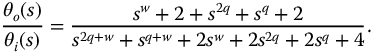
Occasionally, a system may be found that cannot be (exactly) expressed as a commensurate-order fractional differential equation. The system may be solvable using the fractional exponential and/or fractional trigonometric functions if the non-commensurate terms can be arranged into separate additive terms. Consider the forced response of a system defined by the transfer function

where, for example,  and q is non-commensurate with w. In unfactored form, the transfer function has the expanded form
Furthermore, the related fractional differential equation is

For  a unit impulse, the forced response solution may be directly written from equation (12.65) using equation (12.21) with w = 0, and related constants as

where  ,
,  , and
, and

12.9 Indexed Fractional Differential Equations: Multiple Solutions
In the development of the fractional trigonometric functions, we have been careful to achieve the most general mathematical forms for the trigonometric functions. Specifically, when series terms such as  have been raised to fractional powers we have included the nonprincipal function forms along with the principal function. These functions (see, e.g., equations (9.6) and (9.7)) have been expressed in indexed form, based on the index k.
To maintain the generality discussed earlier, the presence of the k index in the fractional trigonometric functions has also been extended to the determination of the related Laplace transforms (see, e.g., Section 9.4 and Table 9.2). This indexing has also been extended to the fractional calculus-based differintegrals of the fractional trigonometric functions in Section 9.6. Thus, it is clear that differential equations containing fractional-order operators can (mathematically) yield multiple solutions.
Consider the following indexed fractional-order differential equation:

where our interest is the forced response, and thus the equation is not initialized.
This gives rise to the following three nonindexed fractional-order differential equations:


With  , a unit impulse function, the solution to equation (12.69) and by inference (12.70)–(12.72) is given by

Clearly, equation (12.69) has associated with its multiple solutions represented by equation (12.73) and by the individual equations (12.70)–(12.72).
The three solutions are shown graphically in Figure 12.1, where  and
and  . The responses shown in Figure 12.1 are for equations (12.70)–(12.72), also for all three values of k from equation (12.73). We can see that the non-zero responses occur in a symmetric pair: k = 0, k = 1. Clearly, all provide legitimate solutions for equation (12.69). The issue of multiple solutions for fractional-order differential equations has been studied by other investigators, for example, Ibrahim and Momani [55].

Figure 12.1 Multiple solutions, x(t), for equation (12.69), given by equations (12.70, k = 0), (12.71, k = 1), and (12.72, k = 2). a = 1,  ,
,  , and
, and  .
.
As a practical matter, when the possibilities of multiple solutions arises in nearly all applications of physical modeling of nature, the combination of boundary and initial conditions provides the path to unique solutions.
An interesting question here is: are there cases in nature where more than a single solution is required to properly describe the physics? One such possibility might be the entanglement of photons emitted as a result of a UV pulse passing through a nonlinear crystal [106]. Such experiments yield responses in which the behavior of the individual elements are symmetric and appear to be “entangled” but may possibly be explained as a multiple (or related) responses sourced by a fractional-order defined field. Multiple paths through nonlinear crystals [31] may also be such a possibility.
12.10 Discussion
This chapter has presented a method for the solution of linear constant-coefficient fractional differential equations of commensurate order. The possible cases of unrepeated, repeated real, and repeated complex poles in the denominator of the characteristic equation were studied and example problems were solved. The methodology is based on the Laplace transforms of the fractional meta-trigonometric functions together with the R-, G-, and H-functions. The G-function provides transforms applicable to fractional differential equations with real fractional repeated poles, while the H-function applies to FDEs with complex fractional repeated poles. The method parallels the method used for the solution of linear ordinary differential equations. Current methods with equations of this type require infinite summations of Mittag-Leffler functions [109], a considerably more difficult approach. A comparison of the two approaches may be found in Ref. [88].
The fractional trigonometric approach provides solutions in the form of real functions as opposed to fractional exponential functions with complex arguments. This allows a direct connection to the physical world.
The fractional meta-trigonometric forms provide important insights and connections to the natural world as is discussed in the application chapters. Finally, because of the indexed nature of the fractional trigonometric functions, the interesting possibility of multiple solutions to physical problems may be investigated.