 xi l/i and in which distance is defined by
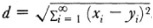
I believe that we lack another analysis properly geometric or linear which expresses location directly as algebra expresses magnitude.
G. W. LEIBNIZ
A number of developments of the nineteenth century crystallized in a new branch of geometry, now called topology but long known as analysis situs. To put it loosely for the moment, topology is concerned with those properties of geometric figures that remain invariant when the figures are bent, stretched, shrunk, or deformed in any way that does not create new points or fuse existing points. The transformation presupposes, in other words, that there is a one-to-one correspondence between the points of the original figure and the points of the transformed figure, and that the transformation carries nearby points into nearby points. This latter property is called continuity, and the requirement is that the transformation and its inverse both be continuous. Such a transformation is called a homeomorphism. Topology is often loosely described as rubber-sheet geometry, because if the figures were made of rubber, it would be possible to deform many figures into homeomorphic figures. Thus a rubber band can be deformed into and is topologically the same as a circle or a square, but it is not topologically the same as a figure eight, because this would require the fusion of two points of the band.
Figures are often thought of as being in a surrounding space. For the purposes of topology two figures can be homeomorphic even though it is not possible to transform topologically the entire space in which one figure lies into the space containing the second figure. Thus if one takes a long rectangular strip of paper and joins the two short ends, he obtains a cylindrical band. If instead one end is twisted through 360° and then the short ends are joined, the new figure is topologically equivalent to the old one. But it is not possible to transform the three-dimensional space into itself topologically and carry the first figure into the second one.
Topology, as it is understood in this century, breaks down into two somewhat separate divisions: point set topology, which is concerned with geometrical figures regarded as collections of points with the entire collection often regarded as a space; and combinatorial or algebraic topology, which treats geometrical figures as aggregates of smaller building blocks just as a wall is a collection of bricks. Of course notions of point set topology arc used in combinatorial topology, especially for very general geometric structures.
Topology has had numerous and varied origins. As with most branches of mathematics, many steps were made which only later were recognized as belonging to or capable of being subsumed under one new subject. In the present case the possibility of a distinct significant study was at least outlined by Klein in his Erlanger Programm (Chap. 38, sec. 5). Klein was generalizing the types of transformation studied in projective and algebraic geometry and he was already aware through Riemann’s work of the importance of homeomorphisms.
The theory of point sets as initiated by Cantor (Chap. 41, sec. 7) and extended by Jordan, Borei, and Lebesgue (Chap. 44, sees. 3 and 4) is not eo ipso concerned with transformations and topological properties. On the other hand, a set of points regarded as a space is of interest in topology. What distinguishes a space as opposed to a mere set of points is some concept that binds the points together. Thus in Euclidean space the distance between points tells us how close points are to each other and in particular enables us to define limit points of a set of points.
The origins of point set topology have already been related (Chap. 46, sec. 2). Fréchet in 1906, stimulated by the desire to unify Cantor’s theory of point sets and the treatment of functions as points of a space, which had become common in the calculus of variations, launched the study of abstract spaces. The rise of functional analysis with the introduction of Hilbert and Banach spaces gave additional importance to the study of point sets as spaces. The properties that proved to be relevant for functional analysis are topological largely because limits of sequences are important. Further, the operators of functional analysis are transformations that carry one space into another.1
As Fréchet pointed out, the binding property need not be the Euclidean distance function. He introduced (Chap. 46, sec. 2) several different concepts that can be used to specify when a point is a limit point of a sequence of points. In particular he generalized the notion of distance by introducing the class of metric spaces. In a metric space, which can be two-dimensional Euclidean space, one speaks of the neighborhood of a point and means all those points whose distance from the point is less than some quantity ε, say. Such neighborhoods are circular. One could use square neighborhoods as well. However, it is also possible to suppose that the neighborhoods, certain subsets of a given set of points, are specified in some way, even without the introduction of a metric. Such spaces are said to have a neighborhood topology. This notion is a generalization of a metric space. Felix Hausdorff (1868-1942), in his Grundzüge der Mengenlehre (Essentials of Set Theory, 1914), used the notion of a neighborhood (which Hilbert had already used in 1902 in a special axiomatic approach to Euclidean plane geometry) and built up a definitive theory of abstract spaces on this notion.
Hausdorff defines a topological space as a set of elements x together with a family of subsets Ux associated with each x. These subsets are called neighborhoods and must satisfy the following conditions:
(a) To each point x there is at least one neighborhood Ux which contains the point x.
(b) The intersection of two neighborhoods of x contains a neighborhood of x.
(c) If y is a point in Ux there exists a Uy such that Uy ⊆ Ux.
(d) If x ≠ y, there exist Ux and Uy such that Ux · Uy = 0.
Hausdorff also introduced countability axioms:
(a) For each point x, the set of Ux is at most countable.
(b) The set of all distinct neighborhoods is countable.
The groundwork in point set topology consists in defining several basic notions. Thus a limit point of a set of points in a neighborhood space is one such that every neighborhood of the point contains other points of the set. A set is open if every point of the set can be enclosed in a neighborhood that contains only points of the set. If a set contains all its limit points, then it is closed. A space or a subset of a space is called compact if every infinite subset has a limit point. Thus the points on the usual Euclidean line are not a compact set because the infinite set of points corresponding to the positive integers has no limit point. A set is connected if, no matter how it is divided into disjoined sets, at least one of these contains limit points of the other. The curve of y = tan x is not connected but the curve of y = sin 1/x plus the interval (— 1, 1) of the Y-axis is connected. Separability, introduced by Fréchet in his 1906 thesis, is another basic concept. A space is called separable if it has a denumerable subset whose closure, the set plus its limit points, is the space itself.
The notions of continuous transformations and homeomorphism can now also be introduced. A continuous transformation usually presupposes that to each point of one space there is associated a unique point of the second or image space and that given any neighborhood of an image point there is a neighborhood of the original point (or each original point if there are many) whose points map into the neighborhood in the image space. This concept is no more than a generalization of the ε — δ definition of a continuous function, the ε specifying the neighborhood of a point in the image space, and the δ a neighborhood of the original point. A homeo-morphism between two spaces S and T is a one-to-one correspondence that is continuous both ways; that is, the transformations from S to T and from T to S are continuous. The basic task of point set topology is to discover properties that are invariant under continuous transformations and homeo-morphisms. All of the properties mentioned above are topological invariants.
Hausdorff added many results to the theory of metric spaces. In particular he added to the notion of completeness, which Fréchet had introduced in his 1906 thesis. A space is complete if every sequence {an} that satisfies the condition that given ε, there exists an N, such that |an — am| < ε for all m and n greater than N, has a limit point. Hausdorff proved that every metric space can be extended to a complete metric space in one and only one way. The introduction of abstract spaces raised several questions that prompted much research. For example, if a space is defined by neighborhoods, is it necessarily metrizable; that is, is it possible to introduce a metric that preserves the structure of the space so that limit points remain limit points? This question was raised by Fréchet. One result, due to Paul S. Urysohn (1898-1924), states that every completely separable normal topological space can be metrized.2 A normal space is one in which two disjoint closed sets can each be enclosed in an open set and the two open sets are disjoined. A related result of some importance is also due to Urysohn. He proved3 that every separable metric space, that is, every metric space in which a countable subset is dense in the space, is homeomorphic to a subset of the Hilbert cube; the cube consists of the space of all infinite sequences {xi} such that 0 xi l/i and in which distance is defined by
The question of dimension, as already noted, was raised by Cantor’s demonstration of a one-to-one correspondence of line and plane (Chap. 41, sec. 7) and by Peano’s curve, which fills out a square (Chap. 42, sec. 5). Fréchet (already working with abstract spaces) and Poincaré saw the need for a definition of dimension that would apply to abstract spaces and yet grant to line and plane the dimensions usually assumed for them. The definition that had been tacitly accepted was the number of coordinates needed to fix the points of a space. This definition was not applicable to general spaces.
In 19124 Poincaré gave a recursive definition. A continuum (a closed connected set) has dimension n if it can be separated into two parts whose common boundary consists of continua of dimension n — 1. Luitzen E. J. Brouwer (1881-1967) pointed out that the definition does not apply to the cone with two nappes, because the nappes are separated by a point. Poincaré’s definition was improved by Brouwer,5 Urysohn,6 and Karl Menger (1902-).7
The Menger and Urysohn definitions are similar and both are credited with the now generally accepted definition. Their concept assigns a local dimension. Menger’s formulation is this: The empty set is defined to be of dimension —1. A set M is said to be n-dimensional at a point P if n is the smallest number for which there are arbitrarily small neighborhoods of P whose boundaries in M have dimension less than n. The set M is called n-dimensional if its dimension in all of its points is less than or equal to n but is n in at least one point.
Another widely accepted definition is due to Lebesgue.8 A space is n-dimensional if n is the least number for which coverings by closed sets of arbitrarily small diameter contain points common to n + 1 of the covering sets. Euclidean spaces have the proper dimension under any of the latter definitions and the dimension of any space is a topological invariant.
A key result in the theory of dimension is a theorem due to Menger (Dimensionstheorie, 1928, p. 295) and A. Georg Nöbeling (1907-).9 It asserts that every n-dimensional compact metric space is homeomorphic to some subset of the (2n + 1)-dimensional Euclidean space.
Another problem raised by the work of Jordan and Peano was the very definition of a curve (Chap. 42, sec. 5). The answer was made possible by the work on dimension theory. Menger10 and Urysohn11 defined a curve as a one-dimensional continuum, a continuum being a closed connected set of points. (The definition requires that an open curve such as the parabola be closed by a point at infinity.) This definition excludes space-filling curves and renders the property of being a curve invariant under homeomorphisms.
The subject of point set topology has continued to be enormously active. It is relatively easy to introduce variations, specializations, and generalizations of the axiomatic bases for the various types of spaces. Hundreds of concepts have been introduced and theorems established, though the ultimate value of these concepts is dubious in most cases. As in other fields, mathematicians have not hesitated to plunge freely and broadly into point set topology.
As far back as 1679 Leibniz, in his Characteristica Geometrica, tried to formulate basic geometric properties of geometrical figures, to use special symbols to represent them, and to combine these properties under operations so as to produce others. He called this study analysis situs or geometria situs. He explained in a letter to Huygens of 167912 that he was not satisfied with the coordinate geometry treatment of geometric figures because, beyond the fact that the method was not direct or pretty, it was concerned with magnitude, whereas “I believe we lack another analysis properly geometric or linear which expresses location [situs] directly as algebra expresses magnitude.” Leibniz’s few examples of what he proposed to build still involved metric properties even though he aimed at geometric algorithms that would furnish solutions of purely geometric problems. Perhaps because Leibniz was vague about the kind of geometry he sought, Huygens was not enthusiastic about his idea and his symbolism. To the extent that he was at all clear, Leibniz envisioned what we now call combinatorial topology.
A combinatorial property of geometric figures is associated with Euler, though it was known to Descartes in 1639 and, through the latter’s unpublished manuscript, to Leibniz in 1675. If one counts the number of vertices, edges, and faces of any closed convex polyhedron—for example, a cube— then V — E + F = 2. This fact was published by Euler in 1750.13 In 1751 he submitted a proof.14 Euler’s interest in this relation was to use it to classify polyhedra. Though he had discovered a property of all closed convex polyhedra, Euler did not think of invariance under continuous transformation. Nor did he define the class of polyhedra for which the relation held.
In 1811 Cauchy15 gave another proof. He removed the interior of a face and stretched the remaining figure out on a plane. This gives a polygon for which V — E + F should be one. He established the latter by triangulating the figure and then counting the changes as the triangles are removed one by one. This proof, inadequate because it supposes that any closed convex polyhedron is homeomorphic with a sphere, was accepted by nineteenth-century mathematicians.
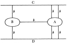
Another well-known problem, which was a curiosity at the time but whose topological nature was later appreciated, is the Koenigsberg bridge problem. In the Pregel, a river flowing through Koenigsberg, there are two islands and seven bridges (marked b in Fig. 50.1). The villagers amused themselves by trying to cross all seven bridges in one continuous walk without recrossing any one. Euler, then at St. Petersburg, heard of the problem and found the solution in 1735.16. He simplified the representation of the problem by replacing the land by points A, B, C, D and the bridges joining them by line segments or arcs and obtained Figure 50.2. The question Euler then framed was whether it was possible to describe this figure in one continuous motion of the pencil without recrossing any arcs. He proved it was not possible in the above case and gave a criterion as to when such paths are or are not possible for given sets of points and arcs.
Gauss gave frequent utterance17 to the need for the study of basic geometric properties of figures but made no outstanding contribution. In 1848 Johann B. Listing (1806-82), a student of Gauss in 1834 and later professor physics at Göttingen, published Vorstudien zur Topologie, in which he discussed what he preferred to call the geometry of position but, since this term was used for projective geometry by von Staudt, he used the term topology. In 1858 he began a new series of topological investigations that were published under the title Der Census räumlicher Complexe (Survey of Spatial Complexes).18 Listing sought qualitative laws for geometrical figures. Thus he attempted to generalize the Euler relation V — E + F = 2.
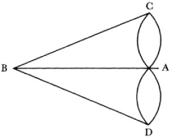
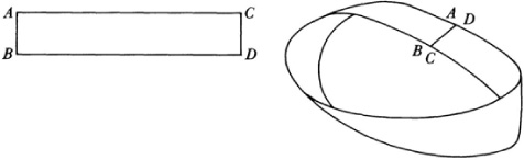
The man who first formulated properly the nature of topological investigations was Möbius, who was an assistant to Gauss in 1813. He had classified the various geometrical properties, projective, affine, similarity, and congruence and then in 1863 in his “Theorie der elementaren Verwandschaft” (Theory of Elementary Relationships)19 he proposed studying the relationship between two figures whose points are in one-to-one correspondence and such that neighboring points correspond to neighboring points. He began by studying the geometria situs of polyhedra. He stressed that a polyhedron can be considered as a collection of two-dimensional polygons, which, since each piece can be triangulated, would make a polyhedron a collection of triangles. This idea proved to be basic. He also showed20 that some surfaces could be cut up and laid out as polygons with proper identification of sides. Thus a double ring could be represented as a polygon (Fig. 50.3), provided that the edges that are lettered alike are identified.
In 1858 he and Listing independently discovered one-sided surfaces, of which the Möbius band is best known (Fig. 50.4). This figure is formed by taking a rectangular strip of paper, twisting it at one short edge through 180°, then joining this edge to the opposite edge. Listing published it in Der Census; the figure is also described in a publication by Möbius.21 As far as the band is concerned, its one-sidedness may be characterized by the fact that it can be painted by a continuous sweep of the brush so that the entire surface is covered. If an untwisted band is painted on one side then the brush must be moved over an edge to get onto the other face. One-sidedness may also be defined by means of a perpendicular to the surface. Let it have a definite direction. If it can be moved arbitrarily over the surface and have the same direction when it returns to its original position, the surface is said to be two-sided. If the direction is reversed, the surface is one-sided.
On the Möbius band the perpendicular will return to the point on the “opposite side” with reverse direction.
Still another problem that was later seen to be topological in nature is called the map problem. The problem is to show that four colors suffice to color all maps so that countries with at least an arc as a common boundary are differently colored. The conjecture that four colors will always suffice was made in 1852 by Francis Guthrie (d. 1899), a little-known professor of mathematics, at which time his brother Frederick communicated it to De Morgan. The first article devoted to it was Cayley’s;22 in it he says that he could not obtain a proof. The proof was attempted by a number of mathematicians, and though some published proofs were accepted for a time, they have been shown to be fallacious and the problem is still open.
The greatest impetus to topological investigations came from Riemann’s work in complex function theory. In his thesis of 1851 on complex functions and in his study of Abelian functions,23 he stressed that to work with functions some theorems of analysis situs were indispensable. In these investigations he found it necessary to introduce the connectivity of Riemann surfaces. Riemann defined connectivity in the following manner: “If upon the surface F [with boundaries] there can be drawn n closed curves a1, a2, …, an which neither individually nor in combination completely bound a part of this surface F, but with whose aid every other closed curve forms the complete boundary of a part of F, the surface is said to be (n + l)-fold connected.” To reduce the connectivity of a surface (with boundaries) Riemann states,
By means of a crosscut [Querschnitt], that is, a line lying in the interior of the surface and going from a boundary point to a boundary point, an (n + l)-fold connected surface can be changed into an n-fold connected one, F″. The parts of the boundary arising from the cutting play the role of boundary even during the further cutting so that a crosscut can pass through no point more than once but can end in one of its earlier points. … To apply these considerations to a surface without boundary, a closed surface, we must change it into a bounded one by the specialization of an arbitrary point, so that the first division is made by means of this point and a crosscut beginning and ending in it, hence by a closed curve.
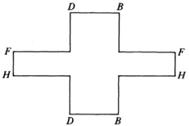
Riemann gives the example of an anchor ring or torus (Fig. 50.5) which is three-fold connected [genus 1 or one-dimensional Betti number 2] and can be changed into a simply connected surface by means of a closed curve abc and a crosscut ab′c′.
Riemann had thus classified surfaces according to their connectivity and, as he himself realized, had introduced a topological property. In terms of genus, the term used by the algebraic geometers of the latter part of the nineteenth century, Riemann had classified closed surfaces by means of their genus р, 2р being the number of closed curves [loop cuts or Rückkehrschnitte] needed to make the surface simply connected and 2р + 1 to cut the surface into two distinct pieces. He regarded as intuitively evident that if two closed (orientable) Riemann surfaces are topologically equivalent they have the same genus. He also observed that all closed (algebraic) surfaces of genus zero, that is, simply connected, are topologically (and con-formally and birationally) equivalent. Each can be mapped topologically on a sphere.
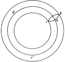
Figure 50.6 Sphere with р holes
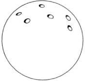
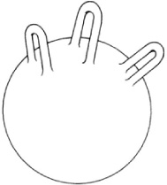
Since the structure of Riemann surfaces is complicated and a topologically equivalent figure has the same genus, some mathematicians sought simpler structures. William K. Clifford showed24 that the Riemann surface of an n-valued function with w branch-points can be transformed into a sphere with р holes where р = (w/2) — n + 1 (Fig. 50.6). There is the likelihood that Riemann knew and used this model. Klein suggested another topological model, a sphere with р handles (Fig. 50.7).25
The study of the topological equivalence of closed surfaces was made by many men. To state the chief result it is necessary to note the concept of orientable surfaces. An orientable surface is one that can be triangulated and each (curvilinear) triangle can be oriented so that any side common to two triangles has opposite orientations induced on it. Thus the sphere is orientable but the projective plane (see below) is non-orientable. This fact was discovered by Klein.26 The chief result, clarified by Klein in this paper, is that two orientable closed surfaces are homeomorphic if and only if they have the same genus. For orientable surfaces with boundaries, as Klein also pointed out, the equality of the number of boundary curves must be added to the above condition. The theorem had been proved by Jordan.27
Figure 50.7 Sphere with р handles
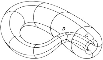
The complexity of even two-dimensional closed figures was emphasized by Klein’s introduction in 1882 (see sec. 23 of the reference in note 25) of the surface now called the Klein bottle (Fig. 50.8). The neck enters the bottle without intersecting it and ends smoothly joined to the base along C. Along D the surface is uninterrupted and yet the tube enters the surface. It has no edge, no inside, and no outside; it is one-sided and has a one-dimensional connectivity number of 3 or a genus of 1. It cannot be constructed in three dimensions.
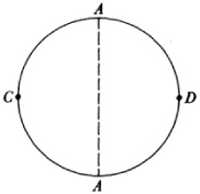
The projective plane is another example of a rather complex closed surface. Topologically the plane can be represented by a circle with diametrically opposite points identified (Fig. 50.9). The infinitely distant line is represented by the semicircumference CAD. The surface is closed and its connectivity number is 1 or its genus is 0. It can also be formed by pasting the edge of a circle along the edge of a Möbius band (which has just a single edge), though again the figure cannot be constructed in three dimensions without having points coincide that should be distinct.
Still another impetus to topological research came from algebraic geometry. We have already related (Chap. 39, sec. 8) that the geometers had turned to the study of the four-dimensional “surfaces” that represent the domain of algebraic functions of two complex variables and had introduced integrals on these surfaces in the manner analogous to the theory of algebraic functions and integrals on the two-dimensional Riemann surfaces. To study these four-dimensional figures, their connectivity was investigated and the fact learned that such figures cannot be characterized by a single number as the genus characterizes Riemann surfaces. Some investigations by Emile Picard around 1890 revealed that at least a one-dimensional and a two-dimensional connectivity number would be needed to characterize such surfaces.
The need to study the connectivity of higher-dimensional figures was appreciated by Enrico Betti (1823-92), a professor of mathematics at the University of Pisa. He decided that it was just as useful to take the step to n dimensions. He had met Riemann in Italy, where the latter had gone for several winters to improve his health, and from him Betti learned about Riemann’s own work and the work of Clebsch. Betti28 introduced connectivity numbers for each dimension from 1 to n — 1. The one-dimensional connectivity number is the number of closed curves that can be drawn in the geometrical structure that do not divide the surface into disjoined regions. (Riemann’s connectivity number was 1 greater.) The two-dimensional connectivity number is the number of closed surfaces in the figure that collectively do not bound any three-dimensional region of the figure. The higher-dimensional connectivity numbers are similarly defined. The closed curves, surfaces, and higher-dimensional figures involved in these definitions are called cycles. (If a surface has edges, the curves must be crosscuts; that is, a curve that goes from a point on one edge to a point on another edge. Thus the one-dimensional connectivity number of a finite hollow tube (without ends) is 1, because a crosscut from one edge to the other can be drawn without disconnecting the surface.) For the four-dimensional structures used to represent complex algebraic functions f (x, y, z) = 0, Betti showed that the one-dimensional connectivity number equals the three-dimensional connectivity number.
Toward the end of the century, the only domain of combinatorial topology that had been rather fully covered was the theory of closed surfaces. Betti’s work was just the beginning of a more general theory. The man who made the first systematic and general attack on the combinatorial theory of geometrical figures, and who is regarded as the founder of combinatorial topology, is Henri Poincaré (1854-1912). Poincaré, professor of mathematics at the University of Paris, is acknowledged to be the leading mathematician of the last quarter of the nineteenth and the first part of this century, and the last man to have had a universal knowledge of mathematics and its applications. He wrote a vast number of research articles, texts, and popular articles, which covered almost all the basic areas of mathematics and major areas of theoretical physics, electromagnetic theory, dynamics, fluid mechanics, and astronomy. His greatest work is Les Méthodes nouvelles de la mécanique céleste (3 vols., 1892-99). Scientific problems were the motivation for his mathematical research.
Before he undertook the combinatorial theory we are about to describe, Poincaré contributed to another area. of topology, the qualitative theory of differential equations (Chap. 29, sec. 8). That work is basically topological because it is concerned with the form of the integral curves and the nature of the singular points. The contribution to combinatorial topology was stimulated by the problem of determining the structure of the four-dimensional “surfaces” used to represent algebraic functions f(x, y, z) = 0 wherein x, y, and z are complex. He decided that a systematic study of the analysis situs of general or n-dimensional figures was necessary. After some notes in the Comptes Rendus of 1892 and 1893, he published a basic paper in 1895,29 followed by five lengthy supplements running until 1904 in various journals. He regarded his work on combinatorial topology as a systematic way of studying n-dimensional geometry, rather than as a study of topological invariants.
In his 1895 paper Poincaré tried to approach the theory of n-dimensional figures by using their analytical representations. He did not make much progress this way, and he turned to a purely geometric theory of manifolds, which are generalizations of Riemann surfaces. A figure is a closed n-dimensional manifold if each point possesses neighborhoods that are homeomorphic to the n-dimensional interior of an n — 1 sphere. Thus the circle (and any homeomorphic figure) is a one-dimensional manifold. A spherical surface or a torus is a two-dimensional manifold. In addition to closed manifolds there are manifolds with boundaries. A cube or a solid torus is a three-manifold with boundary. At a boundary point a neighborhood is only part of the interior of a two-sphere.
The method Poincaré finally adopted appears in his first supplement.30Though he used curved cells or pieces of his figures and treated manifolds, we shall formulate his ideas in terms of complexes and simplexes, which were introduced later by Brouwer. A simplex is merely the n-dimensional triangle. That is, a zero-dimensional simplex is a point; a one-dimensional simplex is a line segment; a two-dimensional simplex is a triangle; a three-dimensional one is a tetrahedron; and the n-dimensional simplex is the generalized tetrahedron with n + 1 vertices. The lower-dimensional faces of a simplex are themselves simplexes. A complex is any finite set of simplexes such that any two simplexes meet, if at all, in a common face, and every face of every simplex of the complex is a simplex of the complex. The simplexes are also called cells.
For the purposes of combinatorial topology each simplex or cell of every dimension is given an orientation. Thus a two-simplex E2 (a triangle) with vertices a0, a1, and a2 can be oriented by choosing an order, say a0a1a2. Then any order of the ai which is obtainable from this by an even number of permutations of the ai is said to have the same orientation. Thus E2 is given by (a0a1a2) or (a2a0a1) or (a1a0a2) or (a2a1a0). Any order derivable from the basic one by an odd number of permutations represents the oppositely oriented simplex. Thus — E2 is given by (a0a2a1) or (a1a0a2) or (a2a1a0).
The boundary of a simplex consists of the next lower-dimensional simplexes contained in the given one. Thus the boundary of a two-simplex consists of three one-simplexes. However, the boundary must be taken with the proper orientation. To obtain the oriented boundary one adopts the following rule: The simplex Ek
a0a1a2…ak
induces the orientation

on each of the (k — l)-dimensional simplexes on its boundary. The  may have the orientation given by (1), in which case the incidence number, which represents the orientation of relative to Ek, is 1, or it may have the opposite orientation, in which case its incidence number is — 1. Whether the incidence number is 1 or —1, the basic fact is that the boundary of the boundary of Ek is 0.
Given any complex one can form a linear combination of its k-dimen-sional, oriented simplexes. Thus if Kki is an oriented ¿-dimensional simplex,

where the ci are positive or negative integers, is such a combination and is called a chain. The numbers ci merely tell us how many times a given simplex
is to be counted, a negative number implying also a change in the orientation of the simplex. Thus if our figure is a tetrahedron determined by four points (a0a1a2a3), we could form the chain C3 = 5 . The boundary of any chain is the sum of all the next lower-dimensional simplexes on all simplexes of the chain, each taken with the proper incidence number and with the multiplicity appearing in (2). Since the boundary of a chain is the sum of the boundaries of each of the simplexes appearing in the chain, the boundary of the boundary of the chain is zero.
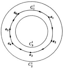
A chain whose boundary is zero is called a cycle. That is, some chains are cycles. Among cycles some are boundaries of other chains. Thus the boundary of the simplex is a cycle that bounds . However, if our original figure were not the three-dimensional simplex but merely the surface, we would still have the same cycle but it would not bound in the figure under consideration, namely, the surface. As another example, the chain (Fig. 50.10)

is a cycle because the boundary of a1 a2, for example, is a2 – a1 and the boundary of the entire chain is zero. But  does not bound any two-dimensional chain. This is intuitively obvious because the complex in question is the circular ring and the inner hole is not part of the figure.
It is possible for two separate cycles not to bound but for their sum or difference to bound a region. Thus the sum (or difference) of  and
and  (Fig. 50.10) bounds the area in the entire ring. Two such cycles are said to be dependent. In general the cycles
  , …,
, …,  are said to be dependent if

bounds and not all the ci are zero.
Poincaré introduced next the important quantities he called the Betti numbers (in honor of Enrico Betti). For each dimension of possible simplexes in a complex, the number of independent cycles of that dimension is called the Betti number of that dimension (Poincaré actually used a number that is 1 more than Beta’s connectivity number.) Thus in the case of the ring, the zero-dimensional Betti number is 1, because any point is a cycle but two points bound the sequence of line segments joining them. The one-dimensional Betti number is 1 because there are one-cycles that do not bound but any two such one-cycles (their sum or difference) do bound. The two-dimensional Betti number of the ring is zero because no chain of two simplexes is a cycle. To appreciate what these numbers mean, one can compare the ring with the circle itself (including its interior). In the latter figure every one-dimensional cycle bounds so that the one-dimensional Betti number is zero.
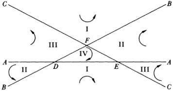
In this 1899 paper, Poincaré also introduced what he called torsion coefficients. It is possible in more complicated structures—for example, the projective plane—to have a cycle that does not bound but two times this cycle does bound. Thus if the simplexes are oriented as shown in Figure 50.11, the boundary of the four triangles is twice the line BB. (We must remember that AB and BA are the same line segment.) The number 2 is called a torsion coefficient and the corresponding cycle BB a torsion cycle. There may be a finite number of such independent torsion cycles.
It is clear from even these very simple examples that the Betti numbers and torsion coefficients of a geometric figure do somehow distinguish one figure from another, as the circular ring is distinguished from the circle.
In his first supplement (1899) and in the second,31 Poincaré introduced a method for computing the Betti numbers of a complex. Each simplex Eq of dimension q has simplexes of dimension q — 1 on its boundary. These have incidence numbers of +1 or — 1. A (q — 1)-dimensional simplex that does not lie on the boundary of Eq is given the incidence number zero. It is now possible to set up a rectangular matrix that shows the incidence numbers of the jth (q — 1)-dimensional simplex with respect to the tth o-dimensional simplex. There is such a matrix Tq for each dimension q other than zero. Tq will have as many rows as there are o-dimensional simplexes in the complex and as many columns as there are (q — 1)-dimensional simplexes. Thus T1 gives the incidence relations of the vertices to the edges. T2 gives the incidence relations of the one-dimensional simplexes to the two-dimensional ones; and so forth. By elementary operations on the matrices it is possible to make all the elements not on the main diagonal zero and those on this diagonal positive integers or zero. Suppose that γq of these diagonal elements are 1. Then Poincaré shows that the q-dimensional Betti number þq (which is one more than Betti’s connectivity number) is
Pq = αq – γq + 1 – γq + 1
where αq is the number of q-dimensional simplexes.
Poincaré distinguished complexes with torsion from those without. In the latter case all the numbers in the main diagonal for all q are 0 or 1. Larger values indicate the presence of torsion.
He also introduced the characteristic N(Kn) of an n-dimensional complex Kn. If this has αk k-dimensional simplexes, then by definition
This quantity is a generalization of the Euler number V — E + F. Poincaré’s result on this characteristic is that if pk is the kth Betti number of Kn then32
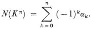
This result is called the Euler-Poincaré formula.
In his 1895 paper Poincaré introduced a basic theorem, known as the duality theorem. It concerns the Betti numbers of a closed manifold. An n-dimensional closed manifold, as already noted, is a complex for which each point has a neighborhood homeomorphic to a region of n-dimensional Euclidean space. The theorem states that in a closed orientable n-dimensional manifold the Betti number of dimension p equals the Betti number of dimension n — p. His proof, however, was not complete.
In his efforts to distinguish complexes, Poincaré introduced (1895) one other concept that now plays a considerable role in topology, the fundamental group of a complex, also known as the Poincaré group or the first homotopy group. The idea arises from considering the distinction between simply and multiply connected plane regions. In the interior of a circle all closed curves can be shrunk to a point. However, in a circular ring some closed curves, those that surround the inner circular boundary, cannot be shrunk to a point, whereas those closed curves that do not surround the inner boundary can be shrunk to a point.
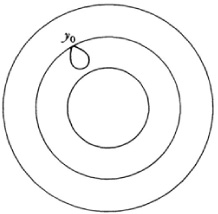
The more precise notion is best approached by considering the closed curves that start and end at a point y0 of the complex. Then those curves that can be deformed by continuous motion in the space of the complex onto each other are homotopic to each other and are regarded as one class. Thus the closed curves starting and ending at y0 (Fig. 50.12) in the circular ring and not enclosing the inner boundary are one class. Those which, starting and ending at y0, do enclose the inner boundary are another class. Those which, starting and ending at y0 enclose the inner boundary n times, are another class.
It is now possible to define an operation of one class on another, which geometrically amounts to starting at y0 and traversing any curve of one class, then traversing any curve of the second class. The order in which the curves are chosen and the direction in which a curve is traversed are distinguished. The classes then form a group, called the fundamental group of the complex with respect to the base point y0. This non-commutative group is now denoted by π1(K, y0) where K is the complex. In reasonable complexes the group does not actually depend upon the point. That is, the groups at y0 and y1, say, are isomorphic. For the circular ring the fundamental group is infinite cyclic. The simply connected domain usually referred to in analysis, e.g. the circle and its interior, has only the identity element for its fundamental group. Just as the circle and the circular ring differ in their homotopy groups, so it is possible to describe higher-dimensional complexes that differ markedly in this respect.
Poincaré bequeathed some major conjectures. In his second supplement he asserted that any two closed manifolds that have the same Betti numbers and torsion coefficients are homeomorphic. But in the fifth supplement33he gave an example of a three-dimensional manifold that has the Betti numbers and torsion coefficients of the three-dimensional sphere (the surface of a four-dimensional solid sphere) but is not simply connected. Hence he added simple connectedness as a condition. He then showed that there are three-dimensional manifolds with the same Betti numbers and torsion coefficients but which have different fundamental groups and so are not homeomorphic. However, James W. Alexander (1888-1971), a professor of mathematics at Princeton University and later at the Institute for Advanced Study, showed34 that two three-dimensional manifolds may have the same Betti numbers, torsion coefficients, and fundamental group and yet not be homeomorphic.
In his fifth supplement (1904), Poincaré made a somewhat more restricted conjecture, namely, that every simply connected, closed, orientable three-dimensional manifold is homeomorphic to the sphere of that dimension. This famous conjecture has been generalized to read: Every simply connected, closed, n-dimensional manifold that has the Betti numbers and torsion coefficients of the n-dimensional sphere is homeomorphic to it. Neither Poincaré’s conjecture nor the generalized one has been proven.35
Another famous conjecture, called the Hauptvermutung (most important conjecture) of Poincaré, asserts that if T1 and T2 are simplicial (not necessarily straightedged) subdivisions of the same three-manifold, then T1 and T2 have subdivisions that are isomorphic.36
The problem of establishing the invariance of combinatorial properties is to show that any complex homeomorphic to a given complex in the point set sense has the same combinatorial properties as the given complex. The proof that the Betti numbers and torsion coefficients are combinatorial invariants was first given by Alexander.37 His result is that if K and K1 are any simplicial subdivisions (not necessarily rectilinear) of any two homeomorphic (as point sets) polyhedra P and P1, then the Betti numbers and torsion coefficients of P and P1 are equal. The converse is not true, so that the equality of the Betti numbers and torsion coefficients of two complexes does not guarantee the homeomorphism of the two complexes.
Another invariant of importance was contributed by L. E. J. Brouwer. Brouwer became interested in topology through problems in function theory. He sought to prove that there are 3g — 3 classes of conformally equivalent Riemann surfaces of genus g > 1 and was led to take up the related topological problems. He proved38 the invariance of the dimension of a complex in the following sense: If K is an n-dimensional, simplicial subdivision of a polyhedron P, then every simplicial subdivision of P and every such division of any polyhedron homeomorphic to P is also an n-dimensional complex.
The proofs of this theorem, as well as Alexander’s theorem, are made by using a method due to Brouwer,39 namely, simplicial approximations of continuous transformations. Simplicial transformations (simplexes into simplexes) are themselves no more than the higher-dimensional analogues of continuous transformations, while the simplicial approximation of continuous transformations is analogous to linear approximation applied to continuous functions. If the domain in which the approximation is made is small, then the approximation serves to represent the continuous transformation for the purposes of the invariance proofs.
Beyond serving to distinguish complexes from one another, combinatorial methods have produced fixed point theorems that are of geometric significance and also have applications to analysis. By introducing notions (which we shall not take up) such as the class of a mapping of one complex into another40 and the degree of a mapping,41 Brouwer was able to treat first what are called singular points of vector fields on a manifold. Consider the circle S1, the spherical surface S2, and the n-sphere 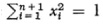 in Euclidean (n + 1)-dimensional space. On S1 it is possible to have a tangent vector at each point and such that the lengths and directions of these vectors vary continuously around the circle while no vector has length zero. There is, one says, a continuous tangent vector field without singularities on S1. However, no such field can exist on S2. Brouwer proved42 that what happens on S2 must happen on every even-dimensional sphere; that is, no continuous vector field can exist on even-dimensional spheres, so that there must be at least one singular point.
Closely related to the theory of singular points is the theory of continuous transformations of complexes into themselves. Of special interest in such transformations are the fixed points. If we denote by f (x) the transform of a point x under such a transformation, then a fixed point is one for which f(x) = x. We may for any point x introduce a vector from x to f(x). In the case of a fixed point the vector is indeterminate and the point is a singular point. The basic theorem on fixed points is due to Brouwer.43 It applies to the n-dimensional simplex (or a homeomorph of it) and states that every continuous transformation of the n-simplex into itself possesses at least one fixed point. Thus a continuous transformation of a circular disc into itself must possess at least one fixed point. In the same paper Brouwer proved that every one-to-one continuous transformation of a sphere of even dimension into itself that can be deformed into the identity transformation possesses at least one fixed point.
Shortly before his death in 1912, Poincaré showed44 that periodic orbits would exist in a restricted three-body problem if a certain topological theorem holds. The theorem asserts the existence of at least two fixed points in an annular region between two circles under a topological transformation of the region that carries each circle into itself, moving one in one direction and the other in the opposite direction while preserving the area. This last “theorem” of Poincaré was proved by George D. Birkhoff.45
Fixed point theorems were generalized to infinite-dimensional function spaces by Birkhoff and Oliver D. Kellogg in a joint paper46 and applied to prove the existence of solutions of differential equations by Jules P. Schauder (1899-1940),47 and by Schauder and Jean Leray (1906-) in a joint paper.48 A key theorem used for such applications states that if T is a continuous mapping of a closed, convex, compact set of a Banach space into itself, then T has a fixed point.
The use of fixed point theorems to establish the existence of solutions of differential equations is best understood from a rather simple example. Consider the differential equation

in the interval 0 ≤ x ≤ 1 and the initial condition y = 0 at x = 0. The solution φ(x) satisfies the equation
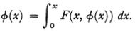
We introduce the general transformation
where f(x) is an arbitrary function. This transformation associates f with g and can be shown to be continuous on the space of continuous functions f(x) defined on [0, 1]. The solution φ that we seek is a fixed point of that function space. If one can show that the function space satisfies the conditions that validate a fixed point theorem, then the existence of φ is established. The fixed point theorems applicable to function spaces do precisely that. The method illustrated by this simple example enables us to establish the existence of solutions of nonlinear partial differential equations that are common in the calculus of variations and hydrodynamics.
The ideas of Poincaré and Brouwer were seized upon by a number of men who have extended the scope of topology so much that it is now one of the most active fields of mathematics. Brouwer himself extended the Jordan curve theorem.49 This theorem (Chap. 42, sec. 5) can be stated as follows: Let S2 be a two-sphere (surface) and J a closed curve (topologically an S1) on S2. Then the zero-dimensional Betti number of S2 — J is 2. Since this Betti number is the number of components, J separates S2 into two regions. Brouwer’s generalization states that an (n — l)-dimensional manifold separates the n-dimensional Euclidean space Rn into two regions. Alexander50generalized Poincaré’s duality theorem and indirectly the Jordan curve theorem. Alexander’s theorem states that the r-dimensional Betti number of a complex K in the n-dimensional sphere Sn is equal to the (n — r — 1)- dimensional Betti number of the complementary domain Sn — K, r ≠ 0 and r ≠ n — 1. For r = 0 the Betti number of K equals 1 plus the (n — 1)-dimensional Betti number of Sn — K and for r = n — 1 the Betti number of K equals the zero-dimensional Betti number of Sn — K minus l.51 This theorem generalizes the Jordan curve theorem, for if we take K to be the (n — 1)-dimensional sphere Sn–1 then the theorem states that the (n — 1)-dimensional Betti number of Sn”1, which is 1, equals the zero-dimensional Betti number of Sn — Sn–1 minus 1 so that the zero-dimensional Betti number of Sn — Sn ’ Sn – 1 is 2 and divides Sn into two regions.
The definitions of the Betti numbers have been modified and generalized in various ways. Veblen and Alexander52 introduced chains and cycles modulo 2 ; that is, in place of oriented simplexes one uses unoriented ones but the integral coefficients are taken modulo 2. The boundaries of chains are also counted in the same way. Alexander then introduced53 coefficients modulo m for chains and cycles. Solomon Lefschetz (1884-) suggested rational numbers as coefficients.54 A still broader generalization was made by Lev S. Pontrjagin (1908-1960),55 in taking the coefficients of chains to be elements of an Abelian group. This concept embraces the previously mentioned classes of coefficients as well as another class also utilized, namely, the real numbers modulo 1. All these generalizations, though they do lead to more general theorems, have not enhanced the power of Betti numbers and torsion coefficients to distinguish complexes.
Another change in the formulation of basic combinatorial properties, made during the years 1925 to 1930 by a number of men and possibly suggested by Emmy Noether, was to recast the theory of chains, cycles, and bounding cycles into the language of group theory. Chains of the same dimension can be added to each other in the obvious way, that is, by adding coefficients of the same simplex; and since cycles are chains they too can be added and their sum is a cycle. Thus chains and cycles form groups. Given a complex K, to each k-dimensional chain there is a (k — 1)-dimensional boundary chain and the sum of two chains has as its boundary the sum of the separate boundary chains. Hence the relation of chain to boundary establishes a homomorphism of the group Ck(K) of k-dimensional chains into a subgroup Hk-1(K) of the group of (k — 1)-dimensional chains. The set of all k-cycles (k > 0) is a subgroup Zk(K) of Ck(K) and goes under this homomorphism into the identity element or 0 of Ck-1(K). Since every boundary chain is a cycle, Hk–1(K) is a subgroup of Zk–1(K).
With these facts we may make the following definition: For any k ≥ 0, the factor group of Zk(K), that is, the A-dimensional cycles, modulo the subgroup Hk(K) of the bounding cycles, is called the kth homology group of K and denoted by Bk(K). The number of linearly independent generators of this factor group is called the kth Betti number of the complex and denoted by pk(K). The kth homology group may also contain finite cyclic groups and these correspond to the torsion cycles. In fact the orders of these finite groups are the torsion coefficients. With this group-theoretic formulation of the homology groups of a complex, many older results can be reformulated in group language.
The most significant generalization of the early part of this century was to introduce homology theory for general spaces, such as compact metric spaces as opposed to figures that are complexes to start with. The basic schemes were introduced by Paul S. Alexandroff (1896-),56 Leopold Vietoris (1891-),57 and Eduard Cech (1893-1960).58 The details will not be given, since they involve a totally new approach to homology theory. However, we should note that this work marks a step toward the fusion of point set and combinatorial topology.
Bouligand, Georges: Les Définitions modernes de la dimension, Hermann, 1935.
Dehn, M., and P. Heegard: “Analysis Situs,” Encyk. der Math. Wiss., B. G. Teubner, 1907-10, III III, 153-220.
Franklin, Philip: “The Four Color Problem,” Scripta Mathematica, 6, 1939, 149-56, 197-210.
Hadamard, J.: “L’Œuvre mathématique de Poincaré, Acta Math., 38, 1921, 203-87.
Manheim, J. H.: The Genesis of Point Set Topology, Pergamon Press, 1964.
Osgood, William F.: “Topics in the Theory of Functions of Several Complex Variables,” Madison Colloquium, American Mathematical Society, 1914, pp. 111-230.
Poincaré, Henri: Œuvres, Gauthier-Villars, 1916-56, Vol. 6.
Smith, David E.: A Source Book in Mathematics, Dover (reprint), 1959, Vol. 2, 404-10.
Tietze, H., and L. Vietoris: “Beziehungen zwischen den verschiedenen Zweigen der Topologie,” Encyk. der Math. Wiss., B. G. Teubner, 1914-31, III AB13, 141-237.
Zoretti, L., and A. Rosenthal: “Die Punktmengen,” Encyk. der Math. Wiss., B. G. Teubner, 1923-27, II C9A, 855-1030.