APPENDICES
APPENDIX A: MATHEMATICAL METHODS
Most of the problems in this book require mathematics that is no more advanced than standard algebra or first-year calculus. We have found, however, that students often need a refresher in some of these basics to boost their confidence. We strongly urge you to use the problems in this text as an excuse to dust off your old math books and get some practice. If you do not already own a handbook of standard functions or a guide to mathematical methods in the sciences, you should probably add one to your shelf. We have found Burington (1973), Dence (1975), Boas (1984), and Potter and Goldberg (1997) to be particularly useful.
This short appendix is intended to introduce a few concepts not generally included in math courses required for the geology curriculum, but that are very useful in geochemistry. We do not pretend that it is an in-depth presentation; our goal is purely pragmatic. Each of these topics appears in one or more of the problems in this text, and should become familiar as you advance in geochemistry.
Partial Differentiation
If a function f has values that depend on only one physical parameter, x, then you know from your first calculus course that the derivative, df(x)/dx, represents the rate of change of f(x) with respect to x. In graphical terms, df(x)/dx (if it exists in the range of interest) is the instantaneous slope of the curve defined by y = f(x). Strictly, df(x)/dx is given by:
df(x)/dx = limh→0 [(f(x + h) − f(x))/h].
Equations involving rates of change in the physical world are extremely common, but it is rare to find one in which the value of the function f depends on only one parameter. More commonly, we deal with f(x, y, z, . . .).
Still, it is useful to know how the function f varies if we change the value of only one of its controlling parameters at a time. For a function f(x, y), for example, we define partial derivatives (∂f(x, y)/∂x)y and (∂f(x, y)/∂y)x by:
(∂f(x, y)/∂x)y = limh→0[(f(x + h, y) − f(x, y))/h],
and
(∂f(x, y)/∂y)x = limh→0 [(f(x, y + h) − f(x, y))/h].
When we write partial derivatives, we use the Greek symbol ∂, rather than d, to remind ourselves that f is a function of more than one variable, and we indicate the variables that are being held fixed by means of subscripts. In chapter 3, for example, we find that the Gibbs free energy (G) of a phase is a function of temperature (T), pressure (P), and the number of moles of each of the components (n1, n2, . . ., ni) in the phase. To consider how G changes as a function of T alone, we look for the value of (∂G/∂T)P,n1,n2 . . ., ni.
Because there can be many interrelationships among variables that describe a system, we can write many different partial derivatives. If pressure, temperature, and volume all influence the state of a system, for example, we may be interested in (∂P/∂T)V, (∂V/∂P)T, (∂T/∂V)P, or any of their reciprocals. These various partial derivatives are not independent of each other. This should be evident from our discussion of the Maxwell relations in chapter 3, in which we investigated some of the relationships among partial derivatives of thermodynamic functions. If that discussion was unfamiliar ground for you, try learning four simple rules for working with partial derivatives. These follow from the standard Chain Rule, which states that if w = f(x, y, z) and if x, y, and z are each functions of u and v, then:
| (∂w/∂u)v |
= (∂w/∂x)y,z (∂x/∂u)v |
|
+ (∂w/∂y)x,z(∂y/∂u)v + (∂w/∂z)x,y(∂z/∂u)v,
(A.1) |
and
(∂w/∂v)u = (∂w/∂x)y,z (∂x/∂v)u + (∂w/∂y)x,z(∂y/∂v)u + (∂w/∂z)x,y(∂z/∂v)u.
(A.2)
The symmetry of the Chain Rule makes it easy to remember. Consider, now, what would happen if we applied the Chain Rule to a function w = f(x, y), in which x was itself a function of y and another variable, z; that is, x = g(y, z). Then:
(∂w/∂z)y = (∂w/∂x)y(∂x/∂z)y + (∂w/∂y)x(∂y/∂z)y,
but
(∂y/∂z)y = 0,
so that:
Rule 1: (∂w/∂x)y(∂x/∂z)y = (∂w/∂z)y.
(A.3)
It can also be shown that:
Rule 2: (∂w/∂x)y = 1/(∂x/∂w)y,
(A.4)
Rule 3: (∂x/∂y)z(∂y/∂z)x(∂z/∂x)y = −1,
(A.5)
and
Rule 4: (∂w/∂y)x = (∂w/∂y)z + (∂w/∂z)y(∂z/∂y)x.
(A.6)
We commonly describe changes in some property of a system by writing differential equations, in which an infinitesimal change df is related to infinitesimal changes in one or more of the variables that control the property. For a function of a single variable, f(x), we can write:
df = (df/dx)dx.
If more than one variable (x, y, z, . . .) can potentially influence the value of f, the equivalent expression is:
| df = |
(∂f/∂x)y,z, . . .dx + (∂f/∂y)x,z, . . .dy |
|
+ (∂f/∂z)x,y . . .dz + . . . . |
The expression on the right side of this equation is called a total differential, because it accounts for the total change df by summing the changes due to each independent variable separately. Consider land elevation, for example, which varies as a function of both latitude and longitude on the Earth’s surface. If you were to move a short distance in some random direction, your total change in elevation would be equal to the slope of the land surface in a north-south direction times the distance you actually moved in that direction, plus the slope in an east-west direction times the distance you moved in that direction.
In many geochemical applications, we find ourselves working with a special type of total differential called an exact or perfect differential. The differentials of each of the energy functions (dE, dH, dF, dG) introduced in chapter 3, for example, belong in this category. To define what we mean, suppose that we know of three properties of a system, each of which is a function of the same set of three independent variables. Identify these properties as P(x, y, z), Q(x, y, z), and R(x, y, z). Can these three properties be related by some function f(x, y, z) in such a way that df = Pdx + Qdy + Rdz? If so, then the expression on the right side is not only the total differential of f, it is also an exact differential. We then say that f is a function of state, with the following particularly useful characteristics:
- Not only are P, Q, and R the partial derivatives of f with respect to x, y, and z, but their own partial derivatives (second derivatives of f) are also interrelated. The following cross-partial reciprocity expressions are true:
| ∂P/∂y)x,z = |
(∂Q/∂x)y,z; |
|
(∂P/∂z)x,y = (∂R/∂x)y,z; (∂Q/∂z)x,y = (∂R/∂y)x,z. |
This property is evident in the Maxwell relations, which derive from the fact that each of the energy functions (E, F, H, and G) is function of state. For example, G = G(P, T, n) = −SdT + VdP + μdn. S(P, T, n), V(P, T, n), and μ(P, T, n), therefore, are like the functions P(x, y, z), Q(x, y, z), and R(x, y, z). Each is a partial differential of G (that is, S = −(∂G/∂T)P,n, V = (∂G/∂P)T,n, and μ = (∂G/∂n)T,P) and the Maxwell relations in this case,
−(∂S/∂P)T,n = (∂V/∂T)P,n = (∂μ/∂n)P,T,
are the cross-partial reciprocity expressions we expect, because G is an exact differential.
- We can determine the total change in f between two states of the system by integrating df between (x1, y1, z1) and (x2, y2, z2) along some reaction pathway, C. An integral of this type is known as a line integral.
For an illustration of how this operation is performed, see worked problem 3.1. When we do this integration for a function of state, we discover that:

Put simply, this means that we always get the same answer, regardless of how we get from state 1 to state 2. The integral of df is said to be independent of path.
- Path independence implies that if we integrate df around a closed loop from state 1 to state 2 and back again, the net change in f will be zero. Again, see worked problem 3.1 to verify that the change in internal energy (an exact differential) around a closed path is zero, whereas the change in either work or heat is not.
Root Finding
It is easy to find the roots of sets of first-order equations by simple algebraic substitution. It is very common, however, to encounter problems in the physical sciences that yield equations in which a key variable x is raised to a higher power or appears in a transcendental function like sin x. A familiar equation from which you learned to extract x when you were in high school is the polynomial:
0 = ax2 + bx + c.
In this example, x can be determined by applying the quadratic formula:

Unfortunately, there are no simple solutions of this type for most equations you will encounter. Adding a cubic term to this polynomial, for example, would make the task of root finding considerably more difficult. There are many ways around this problem, most of which involve a numerical approach instead of a closed-form or analytical one. They are thus well suited to analysis by computer or a pocket calculator. We briefly discuss one of these approaches, the Newton-Raphson method, which is mentioned as a means for solving several problems in chapters 4, 7, and 14.
Consider the curve for the function y = f(x) in figure A.1. Suppose that f(x) has a real root at x = a0 that we want to find. One way to do this would be simply to guess at random successive values of x. If we are patient and watch to see that f(x) is closer to zero with each guess, we will eventually find the value for which f(x) = 0. By examining figure A.1, however, we can see a way to make guesses in a more sophisticated way. Suppose that our first guess is that x = a1, reasonably close to a0 but not correct. The error in this guess is |a1 − a0|, shown by the distance AC in the figure. Assuming that this error is unacceptably large, we now make a better guess by drawing the tangent BP to the curve at point P, and see that the tangent crosses the x axis at x = a2. The error is now only |a2 − a0|, or the distance AB. We repeat the process, each time estimating the improved value of ai+l by drawing a tangent to y = f(x) at the point corresponding to ai, until the error |ai − a0| is acceptably small.
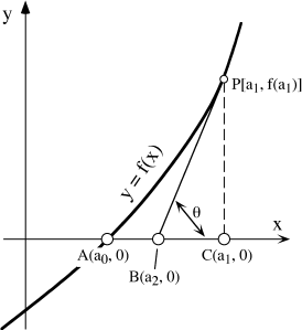
FIG. A.1. Geometric basis for the Newton-Raphson method for finding a root of f (x). Line BP is the tangent to f (x) at point P.
We can write an algorithm to express this method in a way that can be used in a computer program. Comparing the first two guesses geometrically, we see that:
AB = AC − BC,
or
(a2 − a0) = (a1 − a0) − PC/tan θ,
from which a2 = a1 − f(a1)/f′(a1), where f′(a1) is the instantaneous slope of f(x) at a1 (that is, f′(a1) = dy/dx at a1). This simple rule gives us a powerful means for making consecutive guesses, provided that (1) f(x) has a derivative in the vicinity of a0, (2) a1 is reasonably close to a0, so the method doesn’t converge on some other root, and (3) f′(ai+1) is not very close to zero, so that we avoid introducing a large numerical error in ai+1. The algorithm, then, is:
- Make an initial guess, a1, of the root.
- Calculate f(a1) and f′(a1).
- Calculate a better value for the root, a2 = a1 − f′(a1)/f(a1).
- Calculate f(a2).
- If f(a2) is acceptably close to zero, stop. Otherwise, repeat steps (2)−(5) until the root is acceptably close.
You may define “acceptably close” with a specific numerical value, or by noting when f(ai) does not change much from one iteration to the next.
Most texts that discuss the Newton-Raphson method fail to point out how easily it can be applied to systems of equations. Because geochemical problems commonly involve functions of more than one variable, you may find it useful to know how this is done. Suppose that several variables (x1, x2, . . ., xn), related by a set of n independent equations, describe a system. To make life frustrating, each of the equations is a complicated function in which the variables appear in several terms, so that finding the values of x1 − xn by substitution or simple matrix methods is impossible. If each of the functions can be differentiated with respect to each of the variables, however, there is hope for use of the Newton-Raphson method.
As in the simple case above, begin by guessing initial values for x1 through xn. Using these, calculate the numerical values of each of the functions (f1, f2, . . ., fn) and place them in a column vector F. Also, calculate each of the partial derivatives (∂f/∂x) and build a matrix J that looks like this:
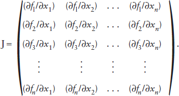
The column vector X = (x1, x2, . . ., xn) can then be found by successive approximations from the matrix version of the Newton-Raphson formula, which we present without proof:
Xk+1 = Xk − (Jk)−1Fk.
This is too cumbersome for a pocket calculator, because it involves inverting the matrix J at each iteration, but it is quite easily done with standard software, such as Microsoft Excel™. An algorithm based on this matrix method tests Fk at each step to see whether each of its elements is acceptably close to zero.
Fitting a Function to Data
In a typical research problem, a geochemist gathers observations on a natural or experimental system and then tries to make sense of the results by looking for functional relationships between the data and system variables that control them. Sometimes the function that best describes the data has a form based on theoretical considerations. At other times, you may choose an empirical function—a polynomial or exponential equation, for example. In any case, the task of fitting that function to your data set involves finding the values of one or more coefficients in the equation so that it gives results that are as close to the observed data as possible.
We demonstrate a common approach to the problem by considering the case in which measured values of some property y appear to depend on some other property x in such a way that a graph of y against x is a straight line. That is, y = f(x) has the form:
y = a0 + a1x.
What values of a0 and a1 are most appropriate for your data? If all of the observed values of y lie precisely on a line, the answer would be easy to find. Unfortunately, however, there are always random errors in any data set, due to sampling technique or undiagnosed complexities in the system (fig. A.2.) The task, then, is to find values of a0 and a1 such that the distance between f(x) and each of the measured values of y is as small as possible. In practice, we generally go one step further and look for a0 and a1 such that the sum of the squares of the deviations from f(x) is minimized. This overall approach, therefore, is known as the method of least squares.
Mathematically, the problem involves minimizing the function:

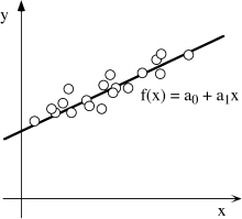
FIG. A.2. The measured values of property x (open circles), in this example, are apparently related to values of property y by some function y = f(x). Because of random errors in the data set, however, the observed values are scattered around the most probable linear function (line).
or, if we have some reason to trust some observations more than others,

where wi is a weighting factor for observation i. The summations are each taken over all values of i from 1 to N, where N is the total number of observations. To minimize Q, we first find expressions for the two partial derivatives of Q with respect to a0 and a1 and set each equal to zero:

and

These can be solved simultaneously to yield:
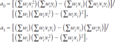
The same procedure can be followed for any polynomial expression.
The Error Function
You are probably somewhat familiar with the function  , where
  . This is the standard form of the normal frequency function, which describes the frequency distribution of events (x) around a mean,
  . The quantity σ is the standard deviation of x, a measure of the spread of values around the mean. This is the “curve” that teachers once used for calculating the grade distribution in classes. It describes the expected distribution of random variations (“errors”) in many other natural situations. In chapter 5 and elsewhere, we have used it indirectly as a means of finding the distribution of mobile ions diffusing across a boundary between adjacent phases.
It can be shown that the area under this curve between zero and some penetration distance x is equal to the probability that an ion lies within that range. This, in fact, is the context in which the normal distribution appears in chapter 5. The error function, erf(x), can be defined as:

and is used to calculate this probability. This form of the error function is commonly used by statisticians. Unfortunately, several other forms are also used by physical scientists. The definition most commonly found in discussions of transport equations is the one we have applied in chapter 5:

It is a simple matter to relate one form of the error function to another by making an appropriate substitution for t and adjusting the integration limits accordingly. Because several subtly different versions exist, you should always check to see how erf(x) is defined for the particular application you have in mind.
Unfortunately, the integration of e−t2 cannot be performed analytically (that is, in neat, closed form). Because erf(x) is a widely used function, however, there are many popular ways to evaluate it. The easiest is simply to look it up in a table. The error function and its complement, erfc(x) = 1 − erf(x), are tabulated in most standard volumes of mathematical functions (for example, Burington 1973). There are also many approximate solutions that are reliable for calculations with pencil and paper. One that yields <0.7% error is the function  . In most applications today, however, erf(x) is calculated by numerical integration.
REFERENCES
Boas, M. L. 1984. Mathematical Methods in the Physical Sciences: Solutions of Selected Problems, 2nd ed. New York: Wiley.
Burington, R. S. 1973. Handbook of Mathematical Tables and Formulas, 5th ed. New York: McGraw-Hill.
Dence, J. B. 1975. Mathematical Techniques in Chemistry. New York: Wiley.
Potter, M. C., and J. Goldberg. 1997. Mathematical Methods for Engineers, 2nd ed. Wildwood: Great Lakes Press.
APPENDIX B: FINDING AND EVALUATING GEOCHEMICAL DATA
Selected Data Sources
The data of geochemical interest are scattered throughout a large number of journals and research reports that focus on the results of narrowly defined studies. In most cases, a search for data on specific systems should begin with the major abstracting journals, Chemical Abstracts and Mineralogical Abstracts, which regularly review the major journals and provide a topical summary of their contents. Limited literature surveys, such as the excellent summary of thermodynamic data sources in Nordstrom and Muñoz (1986), are also useful guides to the primary literature. Rather than provide another survey of this type, here we have compiled a short list of general references that are widely used by geochemists. In almost all cases, these are tabulations or databases built of information gathered from the primary research literature. They offer the advantage of being a quick overview of values that might otherwise be hard to find except in obscure corners of the library. More importantly, a large number of these (but not all!) are critical evaluations of the data, checked for internal consistency.
Using the Data
Before you use the data in any tabulation, be sure to read the text material that accompanies it, describing the criteria for data selection, the reactions that were investigated experimentally to obtain the data, the choice of standard and reference states, and the methods that were used to calculate interpolated, or “derived,” values. Because data are gathered for many purposes, these criteria may not be the same from one source to another. Also, tests for the internal consistency of data compilations may be applied in different ways by various teams of compilers. Therefore, you should not assume that you can safely mix values garnered from different sources in a single problem. For a very good discussion of the potential problems of dealing with multiple data sources, consult chapter 12 of Nordstrom and Muñoz (1986).
Despite these problems, it is usually advisable and often necessary to consult several sources as you compile data for use in your calculations. You will find that teams of researchers have made idiosyncratic choices that emphasize different types of information for the same substances. The JANAF tables (Stull and Prophet 1971 et seq.), for example, indicate the temperatures at which phase changes take place in the substance being reported, but do not indicate phase changes in the reference state elements used to determine  and
and  . Robie and coworkers (1978) report both. In addition, Robie and coworkers provide pairs of tables for silicate minerals that report free energies and enthalpies of formation from both the elements and from the oxides. The JANAF tables, however, include a short summary of the data sources consulted during compilation and, in most cases, a critical justification for the particular choices that were made in preparing their tables. This is a useful feature rarely found in other compendia. Helgeson and colleagues (1978) carry this approach to an extreme by producing a document in which evaluation of the data is the major concern. The data tables are only a few pages of the text and are in a compressed form. It is left to the reader, for example, to calculate thermodynamic values above 298 K by laboriously integrating heat capacity power functions.
Most of the data in standard tabulations should be familiar to students who have read chapters 3, 4, and 9 of this text. The lone exception is the free energy function, defined as  . Values of this function do not change very much with temperature, so that it is usually very safe to interpolate linearly to find values between tabulated temperatures. For reactions among various substances, then, it can be shown that:

so that

where we have followed our convention that quantities with the subscript r are the stoichiometric sum of values for the product phases minus the reactant phases. When the free energy function is available, it serves as a labor-saving alternative to calculating  from heat capacity data and reference state values for enthalpy and entropy.
For those instances when it is preferable to use heat capacity data, it is convenient to have them in the form of a power law. A commonly used expression is:
CP = R(a + bT + cT2 + dT3 + eT4),
in which R (= 1.98726 cal mole−1 K−1) is the gas constant. Robie and coworkers (1978), for example, tabulate values of the constants a, b, c, d, and e for each of the substances in their compendium.
GENERAL REFERENCE
Carmichael, I.S.E., and H. P. Eugster, eds. 1987. Thermodynamic Modeling of Geological Materials: Minerals, Fluids and Melts. Reviews in Mineralogy 17. Washington, D.C.: Mineralogical Society of America.
DeBievre, P., M Gallet, N. E. Holden, and I. L. Barnes. 1984. Isotopic abundances and atomic weights of the elements. Journal of Physical and Chemical Reference Data 13:809–891.
Greenwood, N. N., and A. Earnshaw. 1997. Chemistry of the Elements, 2nd ed. Oxford: Pergamon.
Li, Y.-H. 2000. A Compendium of Geochemistry. Princeton: Princeton University Press.
Lide, D. R., ed. 2001. CRC Handbook of Chemistry and Physics, 81st ed. Boca Raton: CRC.
Nordstrom, D. K., and J. L. Muñoz. 1986. Geochemical Thermodynamics. Malden: Blackwell.
Ronov, A. B., and A. A. Yaroshevsky. 1969. Chemical composition of the earth’s crust. In P. J. Hart, ed., The Earth’s Crust and Upper Mantle. American Geophysical Union Monograph 13. Washington, D.C.: American Geophysical Union, pp. 35–57.
Wedepohl, K. H., ed. 1969. Handbook of Geochemistry, 2 vols. New York: Springer-Verlag.
ELEMENTS AND INORGANIC COMPOUNDS
Chase, M. W., Jr. 1998. NIST-JANAF Thermochemical Tables, 4th ed. Monograph 9. Journal of Physical and Chemical Reference Data. Washington, D.C.: National Institute of Standards and Technology.
CODATA. 1978. CODATA Recommended Key Values for Thermodynamics 1977. CODATA Bulletin 28. Oxford: Pergamon.
CODATA. 1987. 1986 Adjustment of the Fundamental Physical Constants. CODATA Bulletin 63. Oxford: Pergamon.
Cox, J. D., D. D. Wagman, and V. A. Medvedev, eds. 1989. CODATA Key Values for Thermodynamics. New York: Hemisphere.
Hultgren, R., P. D. Desai, D. T. Hawkins, M. Gleiser, K. K. Kelly, and D. D. Wagman. 1973. Selected Values of the Thermodynamic Properties of Binary Alloys. Metals Park: American Society for Metals.
Merrill, L. 1982. Behavior of the AB2-type compounds at high pressures and high temperatures. Journal of Physical and Chemical Reference Data 11:1005–1064.
Naumov, G. B., B. N. Ryzhenko, and I. L. Khodakovskii. 1974. Handbook of Thermodynamic Data. NTIS Document Pb-226, 722/7CxA. Washington, D.C.: U.S. Department of Commerce.
Parker, V. B., D. D Wagman, and W. H. Evans. 1971. Selected Values of Chemical Thermodynamic Properties: Tables for the Alkaline Earth Elements (Elements 92 through 97 in the Standard Order of Arrangement). U.S. National Bureau of Standards Technical Note 270-6. Washington, D.C.: U.S. Department of Commerce.
Schumm, R. H., D. D. Wagman, S. Bailey, W. H. Evans, and V. B. Parker 1973. Selected Values of Chemical Thermodynamic Properties: Tables for the Lanthanide (Rare Earth) Elements (Elements 62 through 76 in the Standard Order of Arrangement). U.S. National Bureau of Standards Technical Note 270-7. Washington, D.C.: U.S. Department of Commerce.
Stull, D. R., and H. Prophet. 1971. JANAF Thermochemical Tables. U.S. National Bureau of Standards NSRDS-NBS 37. Washington, D.C.: U.S. Department of Commerce.
Supplement 1974 by Chase, M. W., Jr., J. L. Curnutt, A. T. Hu, H. Prophet, and L. C. Walker. Journal of Physical and Chemical Reference Data 3:311–480.
Supplement 1975 by Chase, M. W., Jr., J. L. Curnutt, H. Prophet, R. A. McDonald, and A. N. Syverud. Journal of Physical and Chemical Reference Data 4:1–175.
Supplement 1978 by Chase, M. W., Jr., J. L. Curnutt, R. A. McDonald, and A. N. Syverud. Journal of Physical and Chemical Reference Data 7:793–940.
Supplement 1982 by Chase, M. W., Jr., J. L. Curnutt, J. R. Downey Jr., R. A. McDonald, A. N. Syverud, and E. A. Valenzuela. Journal of Physical and Chemical Reference Data 11:695–940.
Wagman, D. D., W. H. Evans, V. B. Parker, I. Halow, S. M. Bailey, and R. H. Schumm. 1968. Selected Values of Chemical Thermodynamic Properties: Tables for the First Thirty-Four Elements in the Standard Order of Arrangement. U.S. National Bureau of Standards Technical Note 270-3. Washington, D.C.: U.S. Department of Commerce.
Wagman, D. D., W. H. Evans, V. B. Parker, I. Halow, S. M. Bailey, and R. H. Schumm. 1969. Selected Values of Chemical Thermodynamic Properties: Tables for Elements 35 through 53 in the Standard Order of Arrangement. U.S. National Bureau of Standards Technical Note 270-4. Washington, D.C.: U.S. Department of Commerce.
Wagman, D. D., W. H. Evans, V. B. Parker, I. Halow, S. M. Bailey, R. H. Schumm, and K. L. Churney. 1971. Selected Values of Chemical Thermodynamic Properties: Tables for Elements 54 through 61 in the Standard Order of Arrangement. U.S. National Bureau of Standards Technical Note 270-5. Washington, D.C.: U.S. Department of Commerce.
Wagman, D. D., W. H. Evans, V. B. Parker, and R. H. Schumm. 1976. Chemical Thermodynamic Properties of Sodium, Potassium, and Rubidium: An Interim Tabulation of Selected Material. U.S. National Bureau of Standards Interim Report NBSIR 76-1034. Washington, D.C.: U.S. Department of Commerce.
Wagman, D. D., W. H. Evans, V. B. Parker, R. H. Schumm, and R. L. Nuttall. 1981. Selected Values of Chemical Thermodynamic Properties: Compounds of Uranium, Protactinium, Thorium, Actinium, and the Alkaline Metals. U.S. National Bureau of Standards Technical Note 270-8. Washington, D.C.: U.S. Department of Commerce.
Wagman, D. D., W. H. Evans, V. B. Parker, R. H. Schumm, I. Halow, S. M. Bailey, K. L. Churney, and R. L. Nuttall. 1982. The NBS tables of chemical thermodynamic properties: Selected values for inorganic and C1 and C2 organic substances in SI units. Journal of Physical and Chemical Reference Data 11(Suppl. 2):1–392.
MINERALS
Haas, J. L., Jr., G. R. Robinson, and B. S. Hemingway. 1981. Thermodynamic tabulations for selected phases in the system CaO-Al2O3-SiO2-H2O at 101.325 kPa (1 atm) between 273.15 and 1800 K. Journal of Physical and Chemical Reference Data 10:575–669.
Helgeson, H. C., J. M. Delany, H. W. Nesbitt, and D. K. Bird. 1978. Summary and critique of the thermodynamic properties of rock-forming minerals. American Journal of Science 278A:1–229.
Robie, R. A., B. S. Hemingway, and J. R. Fisher. 1978. Thermodynamic Properties of Minerals and Related Substances at 298.15 K and One Atmosphere Pressure and at Higher Temperatures. U.S. Geological Survey Bulletin 1259. Washington, D.C.: U.S. Geological Survey.
Robie, R. A., B. S. Hemingway, and H. T. Haselton. 1983. Thermodynamic Properties of Minerals. U.S. Geological Survey Professional Paper 1375. Washington, D.C.: U.S. Geological Survey.
Robinson, G. R., J. L. Haas Jr., C. M. Schafer, and H. T. Hazelton Jr. 1982. Thermodynamic and Thermophysical Properties of Selected Phases in the MgO-SiO2-H2O-CO2, CaO-Al2O3-SiO2-H2O-CO2, and Fe-FeO-Fe2O3-SiO2 Chemical Systems, with Special Emphasis on the Properties of Basalts and Their Mineral Components. U.S. Geological Survey Open-File Report 83-79. Washington, D.C.: U.S. Geological Survey.
Woods, T. L., and R. M. Garrells. 1987. Thermodynamic Values at Low Temperature for Natural Inorganic Materials. New York: Oxford University Press.
AQUEOUS SPECIES
Burnham, C. W., J. R. Holoway, and N. F. Davis. 1969. Thermodynamic Properties of Water to 1000°C and 10,000 bars. Geological Society of America Special Paper 132. Boulder: Geological Society of America.
Criss, C. M., and J. W. Cobble. 1964. The thermodynamic properties of high temperature aqueous solutions. IV. Entropies of the ions up to 200° and the correspondence principle. Journal of the American Chemical Society 86:5385–5390.
Criss, C. M., and J. W. Cobble. 1964. The thermodynamic properties of high temperature aqueous solutions. V. The calculation of ionic heat capacities up to 200°. Entropies and heat capacities above 200°. Journal of the American Chemical Society 86:5390–5393.
Hamer, W. J. 1968. Theoretical Mean Activity Coefficients of Strong Electrolytes in Aqueous Solutions from 0 to 100°C. U.S. National Bureau of Standards NSRDS-NBS 24. Washington, D.C.: U.S. Department of Commerce.
Helgeson, H. C. 1967. Thermodynamics of complex dissociation in aqueous solution at elevated temperatures. Journal of Physical Chemistry 71:3121–3136.
Helgeson, H. C. 1969. Thermodynamics of hydrothermal systems at elevated temperatures and pressure. American Journal of Science 267:729–804.
Helgeson, H. C. 1982. Errata: Thermodynamics of minerals, reactions, and aqueous solutions at high temperatures and pressures. American Journal of Science 282:1144–1149.
Helgeson, H. C. 1985. Errata II: Thermodynamics of minerals, reactions, and aqueous solutions at high pressures and temperatures. American Journal of Science 285:845–855.
Helgeson, H. C., and D. H. Kirkham. 1974. Theoretical prediction of the thermodynamic behavior of aqueous electrolytes at high pressures and temperatures: I. Summary of the thermodynamic/electrostatic properties of the solvent. American Journal of Science 274:1089–1198.
Helgeson, H. C., and D. H. Kirkham. 1974. Theoretical prediction of the thermodynamic behavior of aqueous electrolytes at high pressures and temperatures. II. Debye-Hückel parameters for activity coefficients and relative partial molal properties. American Journal of Science 274: 1199–1261.
Helgeson, H. C., and D. H. Kirkham. 1976. Theoretical prediction of the thermodynamic behavior of aqueous electrolytes at high pressures and temperatures. III. Equation of state for aqueous species at infinite dilution. American Journal of Science 276:97–240.
Helgeson, H. C., D. H. Kirkham, and G. C. Flowers. 1982. Theoretical prediction of the thermodynamic behavior of aqueous electrolytes at high pressures and temperatures. IV. Calculation of activity coefficients, osmotic coefficients, and partial molal and standard and relative partial molal properties to 600°C and 5 kb. American Journal of Science 281:1249–1516.
Hogfeldt, E. 1982. Stability Constants of Metal Ion Complexes: Part A. Inorganic Ligands. IUPAC Chemical Data Series no. 21. Oxford: Pergamon.
Horne, R. A., ed. 1972. Water and Aqueous Solutions: Structure, Thermodynamics, and Transport Properties. New York: Wiley Interscience.
Sillén, L. G., and A. E. Martell. 1964. Stability Constants of Metal-Ion Complexes. The Chemical Society Special Publication no. 17. London: The Chemical Society. (Supplement 1971.)
REACTION KINETICS
Cohen, N., and K. R. Westberg. 1983. Chemical kinetic data sheets for high-temperature chemical reactions. Journal of Physical and Chemical Reference Data 12:531–590.
PHASE RELATIONS
Brookins, D. G. 1988. Eh-pH Diagrams for Geochemistry. New York: Springer-Verlag.
Ehlers, E. G. 1987. The Interpretation of Geological Phase Diagrams. Mineola: Dover.
Levin, E. M., C. R. Robbins, and H. F. McMurdie. 1964. Phase Diagrams for Ceramists, vol. 1. Columbus: American Ceramic Society.
APPENDIX C: NUMERICAL VALUES OF GEOCHEMICAL INTEREST
Dimensions of the Earth
| Mass of the Earth |
5.973 × 1024 kg |
| Mass of the atmosphere |
5.1 × 10¹⁸ kg |
| Mass of the oceans |
1.4 × 10²¹ kg |
| Mass of the crust |
2.6 × 10²² kg |
| Mass of the mantle |
4.0 × 1024 kg |
| Mass of the outer core |
1.85 × 1024 kg |
| Mass of the inner core |
9.7 × 10²² kg |
| Equatorial radius |
6.378139 × 10⁶ m |
| Polar radius |
6.35675 × 10⁶ m |
| Surface area of the Earth |
5.1 × 10¹⁴ m2 |
| Surface area of the oceans |
3.62 × 10¹⁴ m2 |
| Surface area of the continents |
1.48 × 10¹⁴ m2 |
| Volume of the oceans |
1.37 × 10²¹ 1 |
| Mean depth of the oceans |
3.8 × 10³ m |
| Continental runoff rate |
3.6 × 10¹⁶ 1 yr−1 |
Physical Constants
| Avogadro’s number |
N = 6.022094 × 10¹³ mol−1 |
| Gas constant |
| R | = 1.98717 cal mol−1 K−1 |
|
= 8.31433 J mol−1 K−1 |
|
= 82.06 cm3 atm mol−1 K−1 |
|
| Faraday’s constant |
| F | = 96,487.0 coulomb equiv−1 |
|
= 23,060.9 cal volt−1 equiv−1 |
|
| Gravitational constant |
| G | = 6.6732 × 10⁻¹¹ m3 kg−1 sec−2 |
|
= 6.6732 × 10⁻¹¹ nt m2 kg−2 |
|
| Boltzmann’s constant |
k = 1.380622 × 10⁻²³ J K−1 |
| Planck’s constant |
h = 6.626176 × 10⁻³⁴ J sec |
| Base of natural logarithms |
e = 2.71828 |
Conversion Factors
| Distance: |
|
| 1 centimeter (cm) |
= 108 Ångström (Å)
= 0.3937 inch |
| Time: |
|
| 1 year |
= 3.154 × 10⁷ sec |
| Mass: |
|
| 1 gram (g) |
= 2.20462 × 10⁻³ lb |
| 1 atomic mass unit (amu) |
= 1.66054 × 10⁻²⁴ g |
| Temperature: |
|
| Kelvins (K) |
= °C + 273.15
= 5(°F − 32)/9 + 273.15 |
| Pressure (mass length−1 time−1): |
|
| 1 atm |
= 1.013250 × 10⁶ dyne cm−2
= 1.013250 bar
= 1.013250 × 10⁵ pascal (Pa)
= 1.013250 × 10⁵ nt m2
= 14.696 lb in−2 |
| Energy (mass length2 time−1): |
|
| 1 joule (J) |
= 107 erg
= 2.389 × 10⁻¹ cal
= 9.868 × 10⁻¹ liter atm
= 6.242 × 10¹¹ eV
= 2.778 × 10⁻⁷ kWh
= 9.482 × 10⁻⁴ Btu |
| Entropy (mass length2 time−2 deg−1): |
|
| 1 Gibbs |
= 1 cal K−1 |
| Viscosity (mass length−1 time−1): |
|
| 1 poise |
= 1 g sec−1 cm−1
= 1 dyne sec cm−1
= 0.1 Pa sec |
|
| Radioactive decay: |
|
| 1 Curie (Ci) |
= 3.7 × 10¹⁰ sec−1 |
| Logarithmic values: ln x |
= 2.303 log x |
| Units of concentration in solutions: |
|
| Molarity (M) |
= moles liter−1 of solution |
| Normality (N) |
= equiv. liter−1 of solution |
| Molality (m) |
= moles kg−1 of H2O* |
| Parts per million (ppm) |
= g/106 g (= mg/kg) |
*Concentrations are commonly reported in the geochemical literature as millimoles kg−1 of solution. To convert this measure to molal units requires that the density of the solution be known. Except in highly concentrated brines, however, little error is introduced if this difference is ignored.


 , where
  . This is the standard form of the normal frequency function, which describes the frequency distribution of events (x) around a mean,
  . The quantity σ is the standard deviation of x, a measure of the spread of values around the mean. This is the “curve” that teachers once used for calculating the grade distribution in classes. It describes the expected distribution of random variations (“errors”) in many other natural situations. In

 . In most applications today, however, erf(x) is calculated by numerical integration.
 and
and  . Robie and coworkers (1978) report both. In addition, Robie and coworkers provide pairs of tables for silicate minerals that report free energies and enthalpies of formation from both the elements and from the oxides. The JANAF tables, however, include a short summary of the data sources consulted during compilation and, in most cases, a critical justification for the particular choices that were made in preparing their tables. This is a useful feature rarely found in other compendia. Helgeson and colleagues (1978) carry this approach to an extreme by producing a document in which evaluation of the data is the major concern. The data tables are only a few pages of the text and are in a compressed form. It is left to the reader, for example, to calculate thermodynamic values above 298 K by laboriously integrating heat capacity power functions.
 . Values of this function do not change very much with temperature, so that it is usually very safe to interpolate linearly to find values between tabulated temperatures. For reactions among various substances, then, it can be shown that:

 from heat capacity data and reference state values for enthalpy and entropy.