FORESTS, STREAMS, seas, and living reefs are ecological systems, called ecosystems for short. They cover the earth with life and control the geobiosphere. They process energy, materials, and information to support an amazing diversity of species. They are the life support system for humanity. In this chapter, we consider how ecosystems illustrate the principles of self-organization: energy hierarchy, metabolism, spatial concentration, material cycling, and pulsing from chapters 1–4. Understanding mechanisms at the level of ecosystems helps us understand the larger scale of society in later chapters.1
SELECTING BOUNDARIES
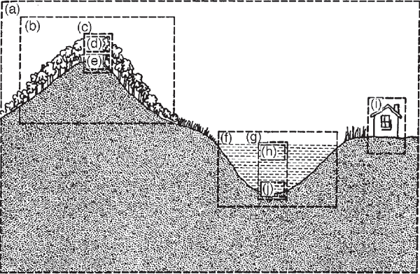
The whole biosphere, its metabolism and circulating materials, was viewed as a single system in fig. 1.3c. Zooming in for a closer view, we see forests, deserts, and seas, which only rarely have distinct boundaries. Looking even closer, we find organisms and nonliving components organized to work together. The biosphere has subsystems within subsystems. What we consider depends on the scale of view. To simplify our study of structure and function, let us define systems by imposing arbitrary boundaries, as in fig. 6.1. Humanity, its machines, its networks of communication, and money circulation, emphasized in later chapters are part of the largest ecosystems and belong in their systems diagrams.
Whereas ecosystems are divided into smaller ecosystems geometrically in fig. 6.1, subsystems may also be separated for study in other ways. Each species’ population can be isolated as a subsystem, which is what happens when human society is considered without nature. Similarly, as illustrated in figs. 2.1 and 2.9, mineral cycles (e.g., carbon, nitrogen, phosphorus, oxygen) can be separated for diagramming and study.
Smaller ecosystems are linked with other ecosystems by the flows of air and water between them and by larger species of animals with territories that include two or more ecosystems. For example, hawks, tigers, and sharks are supported by, and affect, a mosaic of different ecosystems that are adjacent. Seasonally migrating birds nest in one ecosystem and winter in another thousands of miles away. Each species couples its life cycle to each area when there is a pulse of energy support there. Examples are sandpipers on beaches, salmon in estuaries, and whales in the sea.
FIGURE 6.1 Forested mountain, fertile lake, and house with various ecosystems arbitrarily defined according to the purpose of study. (a) An inclusive system with the total landscape included; (b) a forested mountain; (c) a single prism of forest for intensive study; (d) a photosynthetic zone; (e) includes regenerative soil, litter, and anima! zones; (f) a lake as a whole; (g) a vertical prism for representative calculations of some of the main parts of the lake; (h) the euphotic (lighted photosynthetic) zone subsystem; (i) the house, further elaborated in fig. 2.11; and (j) mud and a hypolimnetic subsystem (colder section of a density-stratified aquatic ecosystem).
SILVER SPRINGS ECOSYSTEM
Let’s introduce ecological systems with the river ecosystem in Silver Springs, Florida (Knight 1980; Odum 1955) (fig. 6.2). In large springs where waters flow out of the ground with constant properties, the union of sunlight with clear water containing optimal quantities of nutrients produces fertile beds of waving green bottom plants, covered with diatoms and supporting a food chain of many animals and microorganisms.2
The simplifications we make to understand complex ecosystems such as Silver Springs are called minimodels. When describing systems, nearly everyone explains the organization of parts and processes with words. Sometimes we draw boundaries in the vertical cross-sectional side view, as in fig. 6.1. Sometimes we simplify our view by making a map of main patterns as viewed from above (fig. 6.2a). Sometimes we represent ecosystems with artistic simplification (as in the Elizabeth A. McMahan drawing in fig. 6.2b). Sometimes we tabulate inventories of species.
Energy Systems Model
Using broad pathways for visual effect, fig. 6.2c is a systems view of the main energy flows passing through blocks, each of which represents an important part of the ecosystem. In each block the energy is transformed to higher quality, and much of its availability is used up. The first block contains the plant producers, which in turn contain a photosynthetic section and a block representing the consumer parts of plants. Consumer populations are grouped in one of four stages of consumption. The first (box H) has herbivores, the second stage (box C) has carnivores, and the third (box TC) has top carnivores. There is an organic pool, called detritus (box D), contributed to and used by many species. The organic detritus is important to all the food pathways. This is typical of many ecosystems. Detritus is a mixture of dead organic matter and living bacteria, which transform substances into long-lasting components.
Because species are grouped, such diagrams present a simplified picture of the energy transformations in each stage that upgrade some energy and disperse degraded energy as heat in the various work processes of the populations. The model in fig. 6.2c was historically important in the period when ecologists were learning to compartmentalize (aggregate in boxes) and build minimodels. These six compartments were called trophic levels. Each was further removed from the source of energy, and each step had a drop of about 10% in potential energy in the transformed flow to the next level (downstream in the energy transformation series). Most species usually receive energy contributions from more than one kind of food, including organic pools, animals, plants, and microbes, rather than from just one of these categories. It is possible to classify a species by the food category that is largest in its diet, or one can even assign a part of a species to different boxes.
Emergy Evaluation and Transformities
The protein content and nutritional quality of organic matter increase with the concentrating process down the energy stream. There is chemical diversification in the body structures of these more complex higher animals, and they draw energy from a larger territory and exert greater control within the ecosystem. Quantitative insight related to their quality comes from evaluation of empower and transformities (chapter 4). Figure 6.2d further simplifies the model of the ecosystem retaining the familiar categories of herbivore, carnivore, top carnivore, and detritus. Transformities increase along the energy transformation chain, indicating the higher values and implying greater influence of the top components (Odum 1996).
Production and Respiratory Metabolism, P and R
In fig. 6.2 the Silver Springs ecosystem is further simplified into two sources, two storages, and the flows of energy (fig. 6.2e) and carbon (fig. 6.2f) in the processes of production and respiration, according to the basic plan of ecosystems given in fig. 2.9. Silver Springs and many forest ecosystems, on average, produce more than they consume, exporting some organic matter in runoff downstream. However, most streams have more organic input and consumption than they produce, exporting the inorganic nutrient byproducts downstream.
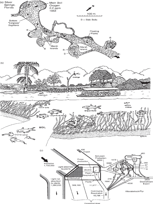
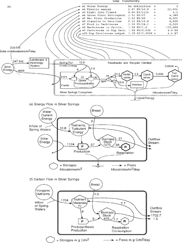
FIGURE 6.2 Summary of energy and material flows in the stream ecosystem of Silver Springs, near Ocala, Florida (Odum 1955). (a) Sketch of headwaters of Silver River; (b) underwater view drawn by Elizabeth A. McMahan (Odum et al. 1998); (c) summary of energy flows (Odum 1955); (d) abbreviated energy diagram of the ecosystem at Silver Springs, Florida, showing the increase of transformities from left to right down the food chain (Collins and Odum 2000); (e) system aggregated into compartments of production and consumption with recycle; (f) aggregate view showing flows of carbon, typical of the nutrient cycles. C, carnivores; D, detritus; H, herbivores; TC, top carnivores.
ECOSYSTEM COMPARISONS
Although ecological systems differ from each other, most have enough features in common to justify describing some basic patterns that are common throughout the world. Although the fishes and plankton of the sea seem very different from the birds and tree leaves of the land system, the energetic properties in the stage diagrams are quite similar. Comparing plankton in the sea with the leaves of the rainforest was a famous thesis of Bates (1960) and Steeman-Nielsen (1957).
The Vertical Design of Ecosystems
If we choose boundaries to include both production (P) and respiration (R), we find the functions stratified in vertical layers as a response to the sunlight entering from above and the action of gravity in separating gas, liquid, and solid phases (fig. 6.3). The photosynthetic production and its chlorophyll-bearing structures become localized on top in the light, and the consumption and larger consumers are concentrated below. Photosynthesis tends to deplete raw materials on top, releasing oxygen and accumulating new organic matter. The top zone receives the sharp diurnal and seasonal pulse of solar insolation and serves as a roof. The organic matter is carried downward by gravity or by the tube systems in the inner bark of tree trunks. Removal of the organics to a lower zone leaves the upper production zone oxidized. The concentration of respiratory action below accumulates carbon dioxide, makes conditions acid, and releases again the mineralized critical nutrients needed by the plants for photosynthesis. This stratum therefore is called the regeneration zone. Oxygen tends to diminish because respiratory metabolism dominates, and in some systems the oxygen reaches zero as other chemically reduced substances form, such as hydrogen, hydrogen sulfide, and ammonia.
Ecosystems have various means for returning regenerated nutrients back up to the photosynthetic production zone. This can occur through root transpiration in trees, through the vertical movements of the swimming or flying consumers who release wastes along the way, by release of gas bubbles that carry absorbed materials to the surface, and through other physical currents to which a particular system is adapted.
In fig. 6.4 ten systems are contrasted, with P and R zones stratified according to the plan in fig. 6.3. The vertical scale ranges from a mile or more in the sea to a few centimeters in mats and encrusting communities. In the thin aquatic systems, the P and R zones are mainly within porous solids (e.g., reef). In systems such as the deep sea, where the solid surface is distant, little organic matter reaches it and only after many years through indirect routes of the deep ocean currents and through successive handling by vertically migrating populations. When the mud surfaces are near the productive euphotic zone, they serve as centers of fuel accumulation and consumption. In general, in aquatic systems more of the circulatory work is done by fluid movements, whereas in land systems specialized plants carry on nongaseous circulation.
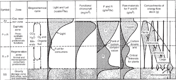
FIGURE 6.3 Principal vertical zones of many ecological systems on land and in water.
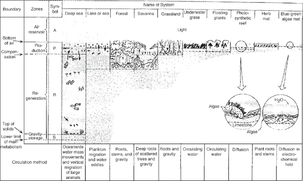
FIGURE 6.4 Vertical zones in 10 contrasting ecological systems defined in fig. 6.3.
Spatial Organization
Ecosystems are spatially organized into centers according to the energy hierarchy (chapter 4, fig. 4.8). Trees are organized about their trunks and animals about their nesting centers. The large size of many animals tends to concentrate the respiratory function, with each organism collecting food over a wide area. Many consumers, such as ants, antelopes, and people, have clustered populations because their complex functions are favored by grouping.
Because incoming solar radiation is spread evenly on an area, photosynthesis and light-absorbing chlorophyll tend to be spread evenly. As we pass from forest to field to swamp and aquatic medium, or to the agricultural systems controlled by humans, there tends to be an even cover of green despite great differences in the kind of plants providing the support. When light intensity is less, plants adapt by increasing the chlorophyll. For instance, cloud-covered Ireland is very green.
Figure 6.5 shows the hierarchical pattern of uniformly spread-out production and clustered consumption. This pattern is observed in diatoms and tube feeders on glass slides that have been submerged in fertile streams for six weeks. It is also observed from an airplane flying at a height of 10,000 feet over the wheat fields (production) and farm villages (consumption) of Kansas. The centralization of tree functions in a forest also follows the pattern, with limbs and roots spreading out from the trunk.
The Functional Biomasses of Nature
Biomass includes the bodies of living organisms and the nonliving organic matter in peat, wood, litter, and sediments. Biomass graphs (fig. 6.6) are pictorial inventory reports that can be used with energy systems diagrams to help describe networks and functions. Obtaining data on biomass representative of the large systems of nature such as forests and seas is a very difficult task that has occupied ecological research for 50 years with thousands of methods. When small spots are studied or small samples taken, the data are not representative because of the spatial organization that is characteristic of most ecosystems. Sampling large sections of systems is laborious and expensive. Figure 6.7 shows a helicopter-borne net, 50 feet in diameter, which the author used in shallow Texas bays to estimate the biomass of fish (Jones et al. 1963). Consistent with the ideal stated as a macroscopic view (chapter 1, fig. 1.2), sampling was done as if by a giant, far above the system, oblivious of the fine-scale variation. Unfortunately, we had no giant.
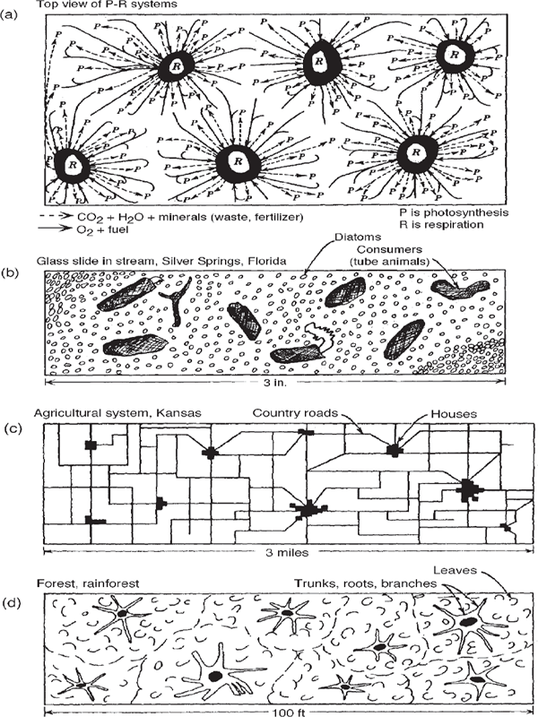
FIGURE 6.5 Patterns of spatial hierarchy in ecological systems viewed from above. (a) Metabolism showing productive photosynthesis (P) dispersed evenly over the surface and respiration (R) clustered in centers and linked to production through convergence of circulating pathways; (b) periphyton in Silver Springs; (c) agrarian landscape from aerial view; (d) canopy and trunks in a tropical rainforest.
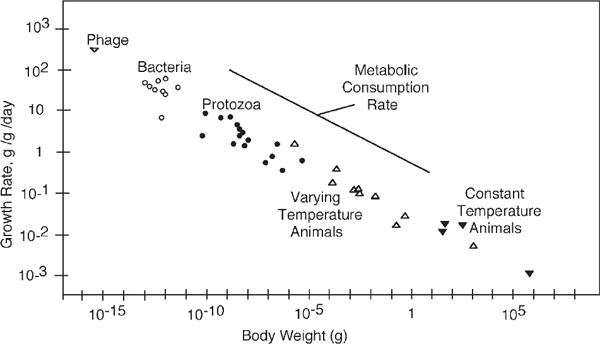
FIGURE 6.6 Growth rate, metabolism, and weight of animals and microorganisms (Straskraba 1966).
Ramon Margalef (1957) and Sven Jorgensen (1997) proposed that maximum biomass was a “goal” of the self-organization of ecosystems in their adaptation and succession. This concept follows from the maximum empower principle because building biomass to a large optimum size is a necessary part of maximizing the productivity of autocatalytic processes (chapter 3, fig. 3.6).
Biomass and Scale
Chapter 4 explained why storage concentrations increase with scale. The biomasses of old-growth trees, elephants, and whales are examples. The larger the territory of support and influence, the larger the stored quantity in the center. For animals, the body biomass is the center of its territory. The larger the unit, the slower the depreciation and turnover time. Energetically, larger concentrations have lower dispersals because of the smaller surface per unit volume. Such units meet the system requirement that higher-quality (higher-transformity) units store longer before sending pulsing feedback control actions out to the surrounding territory.
At first glance the biomass seems to vary widely. A person strolling in a forest sees a great mass of plant matter and a few small animals. From a fishing boat in the sea, usually no plants are visible at all, but large fish appear from time to time. With such different proportions of foliage and creatures, we might conclude that the fundamental bases of these living patterns are different.

FIGURE 6.7 Helicopter-borne drop net ready for release of electromagnetic supports over Corpus Christi Bay, Texas (Jones et al. 1963).
However, the basic photosynthesis in the sea and in the forest is done by tiny cells with rapid turnover times. In lakes and the sea, the water provides the structural support, whereas in the forest, the ecosystem supports the photosynthetic cells with wood structure (leaves, limbs, roots, trunks, and peaty soil components).
The woody storages above ground and soil organics below ground are high in the energy transformation chain, with less energy, slower turnover time, and longer times between pulses and restarts. Perhaps the greatest ecosystem biomass is to be found in the giant trees of virgin rainforest (fig. 6.8) and the great trees of the redwood and sequoia forests of the western United States. These contain huge emergy content because of the hundreds of years of environmental work needed to produce them. In the sea comparable structure is the one or two parts per million organic matter in the huge seawater mass, with similar turnover time to the organics in the forest.
Figure 4.6d and fig. 6.6 are examples of the many published graphs showing the declining unit growth rate and metabolism with scale (Calder 1984; Peters 1983; Zeuthen 1953). This is a property of the universal energy hierarchy explained in chapter 4. At higher hierarchical levels less energy is processed, and there are smaller depreciation rates and greater storage concentrations. Pulsing renewal has greater impact (e.g., when a great tree falls).
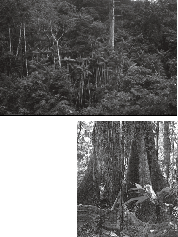
FIGURE 6.8 Large biomass of old-growth rainforest. (a) Virgin forest of Dominica; (b) old growth from Costa Rica.
PHOTOSYNTHETIC PRODUCTION
As explained previously (fig. 2.1, fig. 3.10), photosynthetic production combines sunlight with materials to produce organic matter. Wherever ecosystems are adapted, photosynthesis is greater when there is more sunlight and the necessary materials are unlimited.
Gross production is the first step in transforming solar energy into chemical potential energy. Measuring gross production directly is difficult because products made by photosynthesis are being used up by the plant’s respiration processes at the same time.3 Net production, the difference between the photosynthesis and the concurrent consumption, is usually measured. An index of gross production often is calculated by adding the rate at which organic matter or oxygen is used up in the dark to the rate of net production in the light. Or the rate of carbon dioxide generation at night is added to the carbon dioxide fixed during the day. The efficiency of gross production (energy produced/energy absorbed) in daylight is about 5%. The efficiency is inverse to the light intensity (chapter 7, appendix fig. A4).4
Production in Underwater Ecosystems
For underwater ecosystems, the main inputs are the sun, nutrients such as phosphorus, nitrogen, and potassium, and the physical stirring of the water (caused by wind, downhill flows of water, tides, differences in water density from heating, evaporation and rivers). The sunlight provides the most energy, but when each input is multiplied by its respective transformity and expressed on a common empower basis, solar, physical, and chemical sources are similar.
Models like that shown in fig. 2.4 or intricate physiological methods are required to estimate processes when P and R are nearly balanced and the plant cells small, as in the tropical sea. In tiny cells, more photosynthesis causes an instantaneous increase in respiration in the light (fig. 2.3) and an almost instantaneous drop in respiration after dark. These areas may have high gross production that does not show up in depositions or gaseous exchanges outside the cells. Because of the difficulty measuring gross production, there are still many doubts about the distribution of the basic photosynthetic process over the earth. Most maps of the world’s productivity are based on net production. These show the areas where there are net foods available to other organisms.
Production and Transpiration
In typical woody ecosystems on land, photosynthesis depends on the process of transpiration by which freshwater from rain reaching soils is drawn up the trunks of trees by the evaporation of water through the microscopic stomate holes in leaves. On land, terrestrial plants use the flow of dry air to evaporate water from leaf pores. This creates pressure differences (25 atmospheres or more) between leaves and roots that draw soil water and many nutrients from the ground to the production processes. The sun’s infrared rays and the photons of visible wavelengths used by photosynthesis heat the leaves, increasing the pressure of the leaf’s water vapor and causing it to escape into the air. The winds also renew concentrations of carbon dioxide at the leaf pores, where it diffuses in for photosynthetic production of organic matter. In other words, terrestrial plants use atmospheric inputs including the sun, turbulent energy, dry air, carbon dioxide, and rainfall, all coupled together as shown in the systems model in fig. 6.9a. Because transpiration integrates all these inputs, it is proportional to net production of terrestrial ecosystems, as shown by Rosenzweig in fig. 6.9b.
Biomes and Productivity
In the grand view of the biosphere, the environment has many spatial subdivisions: seas, tundras, deserts, and great rivers. Several generations of observers have thought that division boundary lines could be drawn to group together systems with similar structure and function called biomes. Thus the areas of coniferous forest of the colder regions have been grouped together, even though the conditions and actual species of plants and animals constituting the system on one continent are mostly different from those on another continent.
Because there are many input factors and sequences to which ecosystems adapt, each with specialized species, there are many kinds of ecosystems on Earth. In order to have a simplified global overview, classifications of ecosystem types (biomes) often have been made with only two factors, ignoring temporal sequences. Figure 6.10a shows a popular classification of major terrestrial biomes on a graph of rainfall and temperature on logarithmic coordinates.5 This system was developed to show the major role of transpiration in productivity, where energy for transpiration was in rough proportion to temperature on a logarithmic scale. In other words, fig. 6.10a represents many biomes because rainfall and energy for transpiration (indicated by temperature) are the main emergy sources to which ecosystems organize their functions.
The climatic belts of the earth determine the location of rainfall and the conditions for transpiration (warm dry air). The satellite view of Africa (fig. 6.10b) shows the location of some of the biomes and their climatic conditions. Rainforest is at the equator, where converging winds cause air to rise, form clouds, and generate gentle rainstorms. Seasonal tropical forest (moist forest) is found to the north and south on either side. Next comes the savanna (seasonal grassland with scattered trees). Deserts with little vegetation are around 35° latitude, where the high-pressure zone of the atmospheric circulation causes air to descend, heat by compression, and evaporate clouds.
Much of the energy of the sun, tide, and earth heat goes through the oceans, generating zones of aquatic climate to which ecosystems adapt, developing different kinds of aquatic ecosystems (aquatic biomes), each with distinctive forms of life. The circulation pattern of the sea has gyres and loops that allow characteristic biological communities to remain in about the same place, even though the water is in continuous motion and ultimately intermixes. For example, the blue-water plankton ecosystem in the center of the subtropical oceans occurs in a low-nutrient, clear-water mass that is gently circulating. In many tropical seas where trade winds blow from east to west, plankton migrate up for part of the day, riding with the current to the west. Then at night they descend to lower layers, with undercurrents to the east riding in a reverse direction.
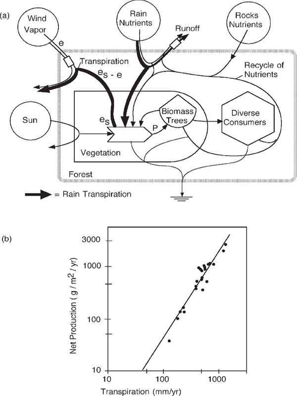
FIGURE 6.9 Transpiration role in terrestrial production. (a) Systems diagram of the role of transpiration in integrating energy sources contributing to photosynthetic production; (b) net production as a function of transpiration in several biomes (Rosenzweig 1968).
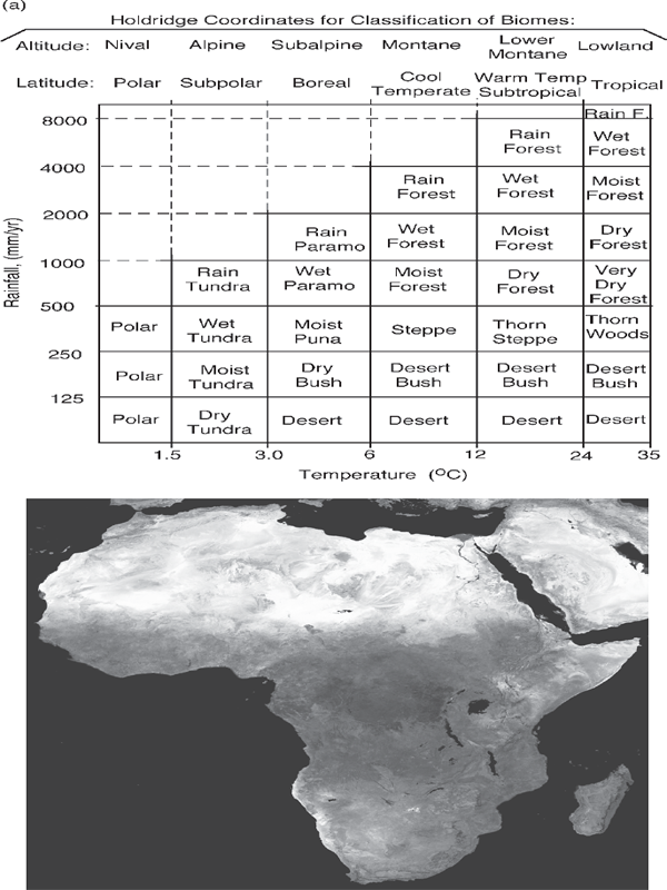
FIGURE 6.10 Holdridge classification of biomes by rainfall and temperature on logarithmic scales. Temperature also represents transpiration, an exponential function of temperature. (b) Satellite view of Africa showing the distribution of main biomes (Tucker et al. 1985).
Underwater biomes include oligohaline estuaries, estuarine oyster reefs, tropical coral reefs, kelp beds, intertidal encrusting communities, hypersaline bays, blue-water plankton systems, blue-green algal mats, seasonally stratified oligotrophic lakes, under-ice marine ecosystems, the chemosynthetic life of undersea volcanic vents, the life in the oceanic deeps, and many others.
Ecosystems in regions with sharp seasons (e.g., arctic seas, monsoon areas of Asia) tend to store production during their growing periods to last during their unproductive periods. These systems demonstrate their productivity by their storages. Systems in steadier surroundings tend to use their production as it is made, and net accumulations are small.
Many of the most fascinating subsystems are uncommon and involve little of the overall budget of the earth. Although not listed as biomes, these subsystems may represent systems that dominated in past ages, systems that will cover the earth in the future, systems that help us visualize possibilities on other planets, systems that can be engineered for the benefit of the economy, and systems that have great value for future scientific progress (see chapter 12). For example, the ancient conical structures found in the geologic record and once thought to be from extinct algal biota were found alive in a coastal environment of modern Australia.
Ultimately, zones occupied by the major subsystems may correspond to climate zones, which determine the amount of available energy and the energetic requirements for adapting to desert, temperate, tropical, and arctic conditions. In naming subsystems of the earth it is informative to choose some physical feature or population that is most prominent and may be said to dominate the emergy flows. The set of input flows expressed on a common empower basis is the ecosystem’s emergy signature.
Comparison of Ecosystem Productivity
Some of the highest and lowest values of production are summarized in table 6.1. The energy flows vary daily and seasonally because the input energies vary in a similar manner. Generally speaking, the seasons of bright light are shorter in the temperate latitudes than in the tropical areas, so the energy input and the power flows are about twice as high in tropical areas (4,000–5,000 kcal/m2/day) as in temperate areas (1,500–4,000 kcal/m2/day). In polar areas the energy input and power flows are smaller (2,000 kcal/m2/day), although they are very intense in the short summer.
TABLE 6.1 Magnitudes of Primary Productiona
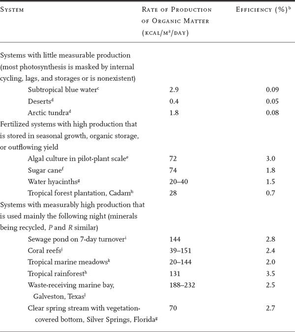
a Day net production plus night respiration. This procedure omits much immediately used photosynthesis. For more detailed data, see general reviews by Pearsall (1954), Ryther (1963), and Westlake (1963). Data that were originally given in grams of oxygen were converted to kilocalories using 4 kcal/g. Data originally given in grams of carbon were converted using 8 kcal/g.
b Percentage of total sunlight received. About half of sunlight is directly involved in photosynthesis, but the heat radiation received may also contribute to such auxiliary processes as evapotranspiration, photorespiration, and rates of biochemical reactions.
c Ryther (1963).
d Rosenzweig (1968).
e Tamiya (1957).
f Odum and E. P. Odum (1959, 1985).
g Odum et al. (1998).
h Odum and Pigeon (1970).
i Ludwig et al. (1951).
j Halfrich and Townsley (1965).
k Odum (1967).
Listed first in table 6.1 are low values characteristic of both land and water in much of the subtropics, where shortages of critical raw materials cause recycling mechanisms to develop. Listed next are net producers cultivated for maximum photosynthesis by inflows of fertilizing nutrients. These values are 100 times higher than those of the limited areas. These systems provide storages and yields for people. Finally, in the third list are some natural ecosystems well organized for effective recycling of minerals by regenerative respiration. They have photosynthetic rates as high as those of the fertilized-yield systems. Only with very intensive fertilization does net production by plants exceed the gross production of diverse, well-organized recycling (example, chapter 12, fig. 12.11).
DIVERSITY
Some ecosystems are simple, with a few species, and others are complex, with many species. In an analogous way, some human societies are simple, with a few occupations, and others are complex, with many occupations. On both scales, more variety means more complexity in the network of energy and material flow. A useful index of diversity is the number of different kinds found in counting 1,000 individuals.6 Table 6.2 contains examples. Whether simple or complex systems develop depends on which generates the maximum metabolism for the conditions (maximum empower principle from chapter 3). Two principles involving productivity explain most of the conditions of diversity observed in nature and microcosms.7
Species Diversity and Physiological Adaptation
The first principle is the complementary allocation of productive energy to physiological function and interspecies organization. When environmental conditions are extreme, the necessary physiological adaptations take more of the energy of the ecosystem’s production, and therefore there are fewer species. For example, brine shrimp have many special enzymes, and estuarine oysters have specially adapted kidneys. Without energy for interspecies organization, competition excludes species. The first examples in table 6.2 are severe environments with few species or occupations.
When environments provide optimal conditions for life, then the species present need not have special physiological abilities. Energy can go into structures and behavior for adapting species to each other. There is more energy to support complex network specializations and more division of labor. The last entries in table 6.2 have more kinds of units and more specialization.
Nature achieves its greatest manifestations of beauty, intricacy, and mystery in the very complex systems: the tropical coral reef, the tropical rainforest, the benthos-dominated marine systems on the west coasts of continents in temperate zones, the bottom of the deep sea, and some ancient lakes of Africa. These places are environmentally stable, and the species networks that develop there have great specialization and division of labor in the same way that the city of New York has enormous diversity of occupations. Complex networks must maintain controls for stability, but there is energy for control because the environments are initially stable, necessitating no great energy expenditures for physiological adaptation.
TABLE 6.2 Species and Occupational Diversity
| SYSTEM | ROLES FOUND WHEN 1,000 INDIVIDUALS ARE COUNTED a |
| Systems with few species in stressed environments | |
| Mississippi Delta, low-salinity zone | 1 |
| Brinesb | 6 |
| Hot springs | 1 |
| Polluted harbor, Corpus Christi, Texas | 2 |
| Humans on a military frontierc | 10 |
| Complex systems in stable environments | |
| Stable stream, Silver Springs, Floridad | 35 |
| Rainforest, El Verde, P.R. | 75 |
| Ocean bottomd | 75 |
| Tropical sead | 90 |
| Human city | 111 |
a When fewer than 1,000 are counted, statistical agreement between duplicate counts is not good; when larger numbers are counted, work is unduly tedious, and discontinuities between different systems tend to be crossed. All units in the same size realm are counted.
b Nixon (1969).
c From Infantry Table of Organization as summarized by Stanton (1991).
d Yount (1956).
d Sanders (1968).
The large and concentrated flows of energy into an industrialized city support extreme specialization of occupational functions not possible for the same number of people in an Eskimo village with climatic stress. Similarly, the rainforest has more circuits than the brine ecosystem. Complexity and diversity on the scale of society thus are related to the flows of energy and the budgeting of these flows between various functions. This principle explains why a decrease in diversity accompanies pollution stress.
In many other environments of Earth the conditions for life vary sharply by day, season, and year. The estuaries of Texas are salty in years of land drought and then are suddenly flooded with freshwater when the rains come. The Mississippi River fluctuates in its pathways to the sea, leaving bays saline at times and fresh in times of high runoff. Sharp seasonal changes occur in the polar tundra, deserts, and waters that receive the fluctuating wastes from human sewers. In these environments energies go into sustaining life against stress and into the constant replacement of decimated stocks. Little energy finds its way to diversification and speciation. The few species that occupy these realms must be generalists.
When energy is channeled into only a few species, there may be large net yields of organic matter instead of the work spent on specialization. The patterns of color, visual cues, and beauty are lacking, but nature is exciting in another way, for the few dominant stocks of creatures are characterized by great blooms, pulses, crops, and migrations. Society can secure food yields from this kind of system, but only irregularly. The annual pulse in the high-salinity Laguna Madre of Texas and Mexico is an example of high production but low diversity.
Species Diversity and Unused Resources
The second principle of diversity is the inverse relationship between excess resources for net production and diversity. Where conditions are not extreme, ecosystems have two main diversity regimes for maximizing empower.
• If there are excessive inflows of available resources, light, or nutrients, then there is overgrowth by competitive but poor-quality producers that yield high net production. They do not use much of the products to sustain high-quality, long-lasting structures. The diversity is low. They may grow in steady state, depositing organic matter made with the excess inputs. People may not like soupy green swimming waters, rafts of water hyacinths, or cattail beds because of their low diversity and low-quality structures, but they are nature’s way of dealing with excess nutrients, converting them into high-quality organic storages in sediments. In a recent survey of sites with high nutrients in Puerto Rico, 85 species were found in the role of net producing low-diversity overgrowth (Kent et al. 2000).
• When available resources are not in excess, a high-diversity, cooperative ecosystem develops with efficient recycling that eliminates any limiting factors other than the sun. Structures are longer lasting, with most of the production going into roles that increase gross production and maintenance. High rates of consumption and recycle favor high rates of gross photosynthesis, but there is little net production.
Energy and the Number of Connections
The number of possible connections that require emergy increases rapidly with the number of species (fig. 6.11a). To coexist, either some emergy-using arrangements must be made to prevent interspecies stress and destructive competition, or systems emergy is lost by the interactions. Figures 6.11b and 6.11c show the plant species found with increasing area in the rainforest in Puerto Rico by counting on the ground. In fig. 6.11d, Keitt (1991) shows the increase in recognizable pixels of satellite images with increasing area.
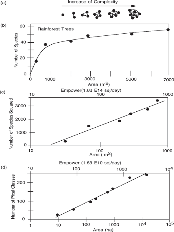
FIGURE 6.11 Emergy and diversity of rainforest. (a) Increase of connection possibilities with numbers of species; (b) plant species found as a function of empower area (Smith 1970); (c) number of species squared; (d) types of rainforest pixels counted from satellite as a function of area and empower (Keitt 1991).
Species–area graphs indicate the area required for a number of species. In many ecosystems the empower (e.g., energy in sun, rain, wind, land) supporting the ecosystem is in proportion to the area. Therefore these graphs can be used to determine how much empower is required to support species diversity (Odum 1999) in the short run. Chapter 8 explains what is required to sustain species information in the long run, and chapter 9 explains the economic valuation of diversity using emdollars.
Biomass and Diversity Minimodels
Principles relating diversity to energy flow are combined in the energy systems diagram in fig. 6.12a. Production is shown generating biomass storage, which then provides an interaction with incoming species to generate a storage tank of diversity (number of species). The extra diversity draws on the biomass storage in proportion to the square of the species number, which limits the diversity. The gross production is increased by the diversity and the efficiency brought by its division of labor. Computer simulation generates the kind of curves of biomass growth and diversity often observed as the succession goes through a stage of simple net production replaced in part with complexity.
Figures 6.12b and 6.12c summarize the net metabolism. The early growth stage has high net production and small respiration, when use of resources is being developed. The later stage has greater gross production and respiration and very little net production. Figure 6.12d is a typical simulation of the minimodel (fig. 6.12a). The rate of net production peaks first, then biomass, and finally diversity.
Oil and Low Diversity of Fossils
When there are only a few poorly organized and unspecialized species, organic matter is not efficiently used, and large quantities go into storage in the sediment and fossil deposits. Thus oil and coal deposits may be related to conditions of severity or fluctuation (e.g., sediments originally formed in hypersaline areas, arctic estuaries, or river mouths). Many of the sedimentary areas of the world carry no oil because they had stable conditions and living networks that were efficient. Recognition of this simple principle can save money spent on oil exploration. Count the species diversity from the little animal skeletons in the drill cuttings of exploratory mining. Possibilities for finding oil are predicted when the species diversity is found to be less than five species per 1,000 animal skeletons counted. Such systems have been observed with high levels of organic matter and residues in their sedimentary depositions.8

FIGURE 6.12 Minimodel called CLIMAX (Odum and Odum 2000) simulating succession in which excess sunlight and nutrients are drawn into use. Appendix fig. A11 has the equations. (a) Energy systems diagram; (b) production and respiration during overgrowth colonization; (c) production and respiration at climax; (d) typical simulation showing the sequence of biomass and diversity.
PATTERNS OVER TIME
Ecosystems, like other systems, pulse with cycles of growth, descent, and restart (chapter 3, fig. 3.13). Metabolism fluctuates in ecosystems even when the conditions of light and temperature are held constant, as in the aquarium ecosystems in experimental growth chambers (fig. 2.6). The small-scale microbial ecosystems with small components rise and restart frequently, in a few hours. The cycles of large forests take centuries. Genetic and ecological changes required for modern coral reefs involve geologic time scales. Within the larger systems with longer cycles there are small-scale components with short-term pulses.
Depending on our scale of view, we call these variations with time oscillations, succession, or evolution. For the same energy, there is more productivity in the long run with pulsing (chapter 3). Some of the timing for pulsing is supplied by the outside energy sources. The inputs of the sun’s energy and other resources rise and fall each day, in seasons each year, and in multiyear cycles. Naturally, photosynthetic production goes up and down with these outside cadences. The ecosystem may adjust its parameters so that the outside frequency maximizes its energy transformations. Or, where the frequency provided by the outside energy sources is not appropriate (wrong scale) for maximum empower, the ecosystems may develop their own internal mechanisms of oscillation.
Prey–Predator Pacemakers
A prey–predator oscillation can serve in ecosystems as a pacemaker (analogous to a heart pacemaker) to provide an appropriate internal pulse.9 Arctic animals, jackrabbits, lynx, and snowy owls are famous for their cycles of abundance and scarcity. Systems models help us understand oscillatory mechanisms. The Lotka–Volterra theory long ago showed how a lag in the eating and being eaten of a prey–predator sequence could create undulations in the stocks (Lotka 1925). Many demonstrations of this principle have been made in laboratory populations in simplified situations in which there were no additional controls. Examples are given by Drake et al. (1966) and Utida (1957) (fig. 6.13). Simulation studies show that minor changes in timing factors can shift a steady system to an oscillating one.10
Successional Sequences
The sequences of succession depend on the starting conditions, outside sources (materials, energy, and species), and scale of time and space. The self-organizational process for microscopic ecosystems can develop its potential in a few days; the largest systems, such as rainforests, and ecosystems that generate land form structures, such as reefs, take centuries. Systems that developed complex steady states were called climaxes in the early studies of ecology. Although mature ecosystems are not permanent (chapter 3, fig. 3.12), the name climax is still appropriate.
Pulsing of Production and Consumption
Ecosystem production and consumption can operate an oscillation by accumulating organics from production and using them with the frenzied pulse of high-transformity consumers described with fig. 3.13. The model in fig. 6.14a (equations in appendix fig. A9) alternates production and consumption and generates the sequence of accumulated organic products and pulsed consumer assets. On a small scale, these pulses are pacemakers within an ecosystem for maximum performance of components. On a larger scale, the rhythm is ecological succession. Total photosynthetic production accumulates living and dead biomass, which is consumed in a frenzied pulse, either from internal mechanisms (episodic fire) or by external destruction from the pulses of the larger-scale system (earthquakes, volcanoes, floods).
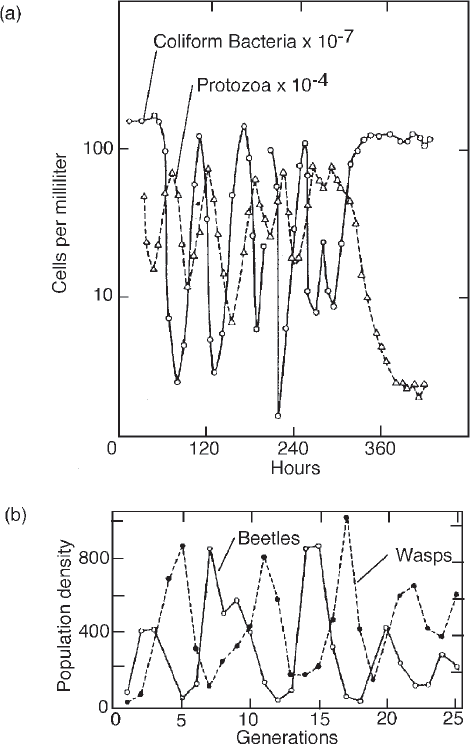
FIGURE 6.13 Example of Lotka-Volterra prey-predator oscillation in laboratory culture. (a) Protozoans eating bacteria (Drake et al. 1966); (b) grain beetles (solid line) and wasps (dashed line) (Utida 1957 from Browning 1963:78).
Figure 6.14b is the result of simulating the minimodel (fig. 6.14a). Net production generates biomass and structure, followed by diversity and efficiency in the typical pattern of succession (fig. 3.12). The stage of low-diversity overgrowth and net production is followed by the climax stage with high-transformity animals, net consumption, and high diversity.
C. S. Holling (1986) provided a figure-eight graph that has been popular for describing ecosystem sequences (fig. 6.14d). The four stages are numbered 1–4, which are comparable with numbers 1–4 in fig. 6.14c.
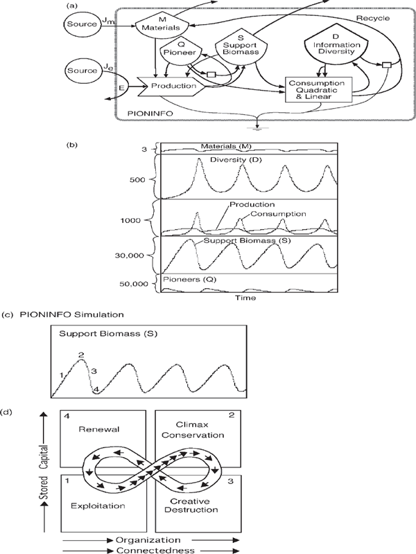
FIGURE 6.14 Pulsing patterns of ecosystem succession, with stage numbers to aid comparisons. (a) Model of production, pulsing, and diversity, called PIONINFO (Odum 1999). See appendix fig. A9 for equations. (b) Typical computer simulation. (c) Points on the graph of biomass that correspond to C. S. Holling’ s 4 stages of the adaptive cycle. (d) C. S. Holling’s figure-8 diagram (Holling 1986; Odum and Odum 1959).
Diurnal Change
Each day ecosystems generate their food and use most of it the next night. This quiet metabolism shows up in the rise and fall of oxygen and carbon dioxide described in chapter 2. For example, the oxygen downstream in Silver Springs (fig. 6.15a) is high in the day and lower at night. By the time the water has gone a kilometer, its properties have been changed by the ecosystem metabolism. The records of metabolism inferred from the oxygen changes and the flow of water at Silver Springs were used to calculate the collective metabolism of the ecosystem. Although the water temperature was constant throughout the year, the production varied with the sunlight, smaller in winter and larger in summer. Although the details are different, diurnal measurements of oxygen under water and carbon dioxide in terrestrial ecosystems are principal ways of calculating their rates of production and consumption.
Figure 6.15b shows the photosynthesis of a coral reef obtained by measuring the change in dissolved oxygen in the waters while flowing across the reef’s complex cover of corals, calcareous algae, and hundreds of animal species.
Figure 6.15c shows the metabolism in a forest that was enclosed in a giant cylinder, with air drawn in at the top and flushed out the bottom with a fan 2 meters in diameter. The sun increased the flow of water from roots up through the trees and out through the microscopic pores in the leaves, the process of transpiration. The photosynthesis and respiration were indicated by the uptake and release of carbon dioxide. Most of the forest respiration was in the soil and lower part of the forest and was accurately measured. The photosynthesis was underestimated because there was some eddy exchange of air out of the cylinder at the top.
The best measurements of land metabolism were made by evaluating the carbon dioxide exchange between forest and atmosphere. In the tropical forest of Samoa the gross primary production was 9.65 g carbon/m2/day (Odum 1995). (See fig. 3.5.)
Seasonal Cycles
The solar energy reaching ecosystems of the earth varies seasonally. Even the equator has a 25% variation in insolation. Most areas have seasonal changes in clouds, winds, and rains. In response, metabolism varies with the seasons. Over much of the world, production and consumption tend to stay in phase, each stimulating the other (fig. 6.16). For example, in the Texas bays (fig. 6.16b) microbial metabolism increases with temperature, and animals migrate in from the sea, using organic matter stored from the previous summer. As a result, respiration increases at the same time as the photosynthesis.
Ecosystems in regimes with sharp seasons (e.g., arctic seas, monsoon areas of Asia) tend to store production during their growing periods to last during their unproductive periods. They show how systems can adapt to the pulsing of the larger-scale surroundings. These systems demonstrate their productivity by their storages. Systems in steadier surroundings tend to use their production as it is made, and net accumulations are small. However, in plankton ecosystems of temperate and arctic waters, the long winter accumulates excess nutrients that set off a bloom of competitive overgrowth in the spring, followed by diversification and a more complex ecosystem later in the summer (fig. 6.17b).
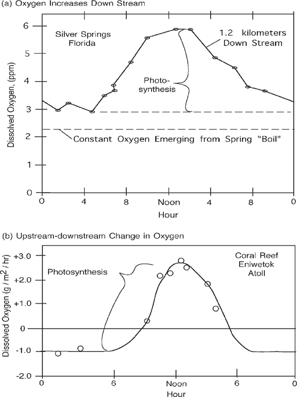

FIGURE 6.15 Diurnal patterns of metabolism in ecosystems. (a) Silver Springs, May 24–25, 1954 (Knight 1980; Odum 1955); (b) interisland coral reef, Japan, Eniwetok, July 1954 (Odum and Odum 1955); (c) metabolism and transpiration in a rainforest enclosed in a giant cylinder, El Verde, Puerto Rico, June 22, 1966 (Odum and Jordan 1970).
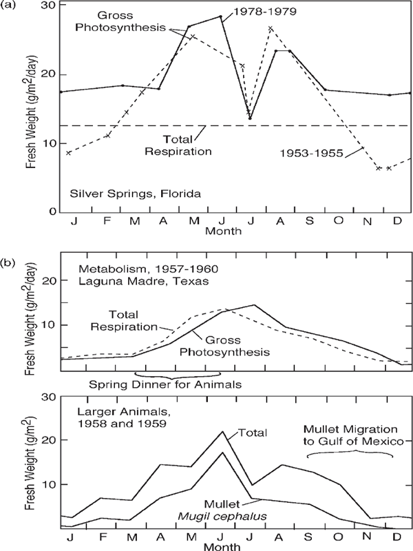
FIGURE 6.16 Seasonal patterns of metabolism and biomass (a) in Silver Springs, Florida; (b) in the Laguna Madre, a high-salinity Texas estuary south of Corpus Christi. Population data were supplied by Thomas Hellier (1962), Arlington College, Texas.
ORGANIZATION OF ECOSYSTEMS
An ecological system is a network of food and mineral flows in which the major pathways are populations of animals, plants, and microorganisms, with each specialized to participate in a different way. Some species of plants and microbes develop different biochemical compounds so that they can be consumed only by consumers that have adapted specialized enzymes. Each species population is isolated by its behavior or chemistry so that its food and mineral flows are not entangled with those of other species. The separation of species keeps the genes separate also. Like wires in a radio, the ecosystem pathways are insulated against short-circuiting. Self-organization with many species allows division of labor that increases efficiency. A system with more species and more organization may be compared to a radio that has more parts. An ecological network of species may involve several hundred different populations.
Power Circuits Versus Controls
Like a radio, an ecosystem has power circuits and control circuits. The abundant species at the base of food chains are the power circuits. Power flows from left to right in systems diagrams.
The higher-transformity consumers at the end of the food web process information and supply control. Higher animals regulate populations, pollinate, plant seeds, place their wastes, and sometimes defend against destructive influences. Squirrels do work of planting acorns in a forest, which is a small part of the forest energy flow, but their work controls the growth of new oaks. On the systems diagrams, such control pathways are drawn from right to left. The principles and diagrams are similar for ecosystems and for people controlling urban power lines (chapter 8).
Color Coding
In a complex ecosystem, as in a complex radio, pathways are color coded with bright colors, which require biochemical energy for pigment synthesis. These colors aid the programs of behavior of organisms with simple nervous systems. People in cities also use color in dress and uniforms, which helps social organization.
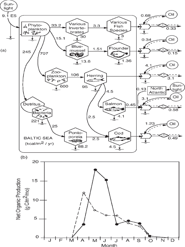
FIGURE 6.17 Ecosystem in the Baltic Sea, from Jansson and Zucchetto (Jansson and Zucchetto 1978; Zucchetto and Jansson 1985). (a) Systems diagram with energy flows; (b) seasonal record of metabolism in the Baltic Sea with photosynthetic spring bloom (solid line) after winter period of respiratory consumption (dashed line) (Stigebrandt 1991).
The many channels with special chemical and physical structures require much metabolic energy for their maintenance. Thus, complex ecosystems have high respiratory metabolism. The power budgets of the whole network are large, but no one product or species receives much energy. Energy goes into the work for the system without piling up offspring, wood, coal, or any other products. Complex systems are very efficient in using all the organic matter they have, leaving little to the fossil record.
Behavior and System Programming
From the ancient lore of natural history, people learn about animals and plants and their life histories, when they breed, how they live and interact, and the meaning of little aspects of their behavior. The sciences of behavior document the facts in a systematic way and describe the various structures and operations. Thus, a male bird with feather movement 1 sets off response 2 in the female, which sets off action 3 in the male, and so on, continuing until reproduction is performed. The process is like a treasure hunt for which we must first fit together the pieces of a map. The treasure is a complex function such as reproduction or nurturing. The sequence of steps forms the same kind of flow chart that a computer programmer draws in explaining the successive steps of a program.
Sometimes we study the interesting patterns of animal behavior as quaint characteristics of nature without recognizing their contributions. We often study single species without asking what the behavior does for the rest of the ecosystem. According to the systems hypothesis of loop reinforcement, the power demands of behavior develop and survive because complex behaviors feed back control services. Complex migrations of crab, shrimp, mullet, and other fishes from the Atlantic coastal bays and estuaries go out to sea in the winter and come back in during the spring, rapidly reinjecting a consumer system as the power input of the sun increases with the warmer weather. Without the migration there would be a lag in development, with much input power unused. The seasonal pulse of production, respiration, and migrating stocks in the shallow Laguna Madre of Texas is shown in fig. 6.16b (Odum 1967).
The eccentric behaviors of birds, bats, and blooms are analogous to preprogrammed computer units that control the timing of computer networks. The huge variety of known species11 is like a bin of electronic parts, tubes, transistors, resistors, and relays. Just as the properties of electronic parts might be listed in a catalog, we need tabulations of the system performances of the earth’s species, including information on such things as storage capacity, power demand, cycle frequencies, and number of input connectors. The design of existing ecological systems will then be better understood, and planning for future designs can begin. In a similar way, the various occupations and operational groups of society constitute a bin of parts for the design of social systems, and the same method may apply.
Up close, observers sometimes see so much beauty and magnificence in details that they can’t see what the species accomplish for the whole. In past cultures, people thought about species as a repatriation from Noah’s ark, God’s handiwork, a service to humanity, or an accidental result of genetic processes operating among islands. But to prevail, species have to contribute somewhere within their system in order to be reinforced by the self-organizing process. The first question for good natural history is, “What does your species do for its system?”; for good anthropology it is, “What does your occupation do for society?”
UNDERSTANDING COMPLEX ECOSYSTEMS
Simplification is required for the human mind to understand such complex systems as rainforests and coral reefs. Some abandon the systems view to study some of the parts or select a chemical substance to follow. Others select simpler ecosystems with fewer species in order to study principles. It is easier to diagram and evaluate the few larger components of the cold Baltic Sea (fig. 6.17) than the more complex systems of tropical seas. Some see ecosystems as an anarchy of species in a competitive struggle for existence without much control. They don’t believe there is any organization to study.
Some study the species and their interactions, but in complex ecosystems this generates more detail than can be collectively understood at the system level. Study of rainforests on islands such as Puerto Rico involves a smaller pool of species than in mainland rainforests. Another approach aggregates species into groups according to main functions, as in the trophic level model in fig. 6.2d. Diagrams such as fig. 6.18 of the montane rainforest in eastern Puerto Rico summarize structure and functions of the rainforest. Even if the same number of units fit on one page, each person makes a different diagram because their different knowledge leads them to select different components to emphasize. However, such diagrams make clear to another person the intended emphasis. Words are too ambiguous and inefficient for representing networks. Having a number of such diagrams helps bring out different patterns and principles.
Others count the species and relate diversity counts to energy support and other factors (fig. 6.11). Some develop large, complex computer models, looking for synthesis to emerge from the combinations. Others keep their computer simulation models simple, like controlled experiments, examining a few features while aggregating the rest (figs. 6.12 and 6.14a).
Zooming the human mind to a larger scale bypasses ecosystem complexity. The ecosystems become units to be described with holistic measures such as total number of species, total biomass, total information, total DNA, total photosynthesis, total respiration, total chlorophyll, overall efficiency of light conversion, energy balance, or chemical cycles. However, all scales are important and interesting, although most scientists concentrate on one scale. By definition, complex ecosystems cannot be understood by study at one scale. Energy systems diagrams are helpful because they show connections between small scales on the left and larger scales to the right. Ecosystem diagrams represent the energy hierarchy.
ORGANIZATION IN THE COMPLEX RAINFOREST
Tracing pathways on the systems diagram of a rainforest (fig. 6.18) helps guide discussion to interesting properties. One can start by pointing to the outside sources from the climate and the earth. Complex rainforests are found where the climate does not have a sharp pulse in drought, temperature, or other factors that force a system to start over each year. Photosynthesis (gross production) is about 32 g dry matter/m2/day. The plant photosynthesis is divided between many different species, each of which has a similar photosynthetic function but is made distinctive by special chemical insulating agents. The cycle for discarding old leaves and recycling minerals is provided by fungi and bacteria, with species adapted to deal with the special chemistry. Various arrangements of roots and microorganisms at the ground level further organize closed-loop mineral cycles, which are mutually stimulating.
Both the producers and the microorganisms are regulated by specialized consumers. Leaf-eating insects are adjusted in their actions to take about 7% of the leaf matter, as long as each plant species is evenly dispersed. Similarly, a great many species of small fungus-eating flies and other small consumers may keep the microorganisms from becoming too numerous. Both the leaf-grazers and the microbe eaters are specialized to deal with the chemical insulating compounds of plants. As long as the various plants are dispersed in small numbers for each species, the plant and microbe eaters cannot find enough continuous specialized food to become epidemic. If any species of plant starts to accelerate its relative growth and become dominant, it will be counterattacked by accelerating actions of the consumers, whose small size gives them a rapid response time. Thus diversity and a check-and-balance system prevent epidemics and maintain stability, a theory supported by much evidence (Voute 1963).
Higher-level consumers, such as the lizards and frogs, and secondary-level microorganisms and eaters of detritus, such as the earthworms, need less chemical specialization because they are not eating the organisms with special chemical insulators. Instead, they are eating the small animal consumers that are not so different in chemical composition. Thus food lines converge, with the higher consumers shifting from one species to another if any become numerous. The convergence also provides a variety of chemical molecules, supplying more complex nutrition, which, in turn, allows the more complex functions and tight packaging required for the rapid movements, elaborate behavioral adaptations, and diversity of the higher organisms. The specialization in higher organisms permits complex patterns of system control, through pollination and seeding.
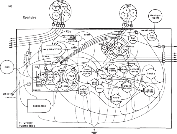
FIGURE 6.18 Ways of thinking about rainforest diversity. (a) Energy systems diagram of guilds and pathways at El Verde, Puerto Rico (Odum 1995); (b) location of some systems functions. Invert., invertebrates; Micro., microbes.
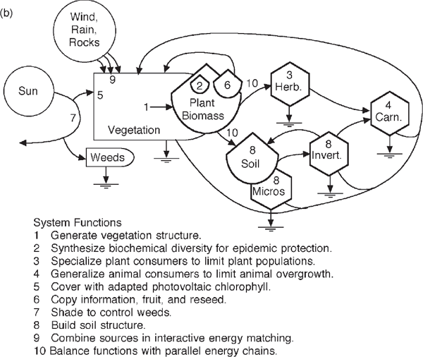
Ultimately, food chain convergence leads to larger birds, mammals, and humans, providing nutritive diversity. The energies of photosynthesis, through dozens of different species, support the work processes of the system, such as light use, duplication, mineral cycling, epidemic stabilization, structural organization, and soil repair. Some of the functions of the various parts of ecosystems are shown in fig. 6.18b. Purposeful mechanisms are self-organized into a decentralized program of ecosystem control. Thus the ancient ecological systems continue on quietly, efficiently, cleanly self-controlled year after year despite impacts and extinctions.
SUMMARY
In this chapter we examined the structure and functions of ecosystems and their energy basis. After a billion years of evolution, our biosphere has many kinds of ecological systems, each adapted to different environmental conditions and each with adaptive mechanisms. The common characteristics of ecosystems were introduced using the stream ecosystem of Silver Springs as an example. Then similarities between ecosystems were found in vertical stratification, spatial organization, temporal sequences, and energy transformation series. Biomass distribution and its metabolism were related to the energy hierarchy. Diversity was found to depend on the allocation of production according to availability of excess resources for net production overgrowth and the priority for physiological adaptation. Patterns over time adapt to external rhythms and internal pacemakers as needed to pulse for maximizing empower. Pulsing cycles are called oscillation, succession, and evolution, depending on the scale. Ways of understanding complex systems were reviewed using the rainforest as an example and network diagrams to clarify the connections between scales. Many similarities exist between complex ecosystems and complex societies, whose energy basis is considered next.
BIBLIOGRAPHY
Note: An asterisk denotes additional reading.
Bates, M. 1960. The Forest and the Sea. New York: Random House.
Beyers, R. J. and H. T. Odum. 1993. Ecological Microcosms. New York: Springer-Verlag.
Browning, T. P. 1963. Animal Populations. New York: Harper & Row.
Calder, W. A. III. 1984. Size, Function, and Life History. Cambridge, MA: Harvard University Press.
Campbell, D. 1984. Energy filter properties of ecosystems. Ph.D. dissertation, University of Florida, Gainesville.
*Clarke, G. L. 1946. Dynamics of production in a marine area. Ecological Monographs, 16: 321–335.
Collins, D and H. T. Odum. 2000. Calculating transformities with an eigenvector method. In M. T. Brown, ed., Emergy Synthesis: Theory and Applications of the Emergy Methodology, Proceedings of the First Biennial Emergy Analysis Research Conference Sept. 1999. Gainesville, FL: Center for Environmental Policy.
Drake, J. F., J. L. Jost, A. G. Frederickson, and J. M. Tsuchiya. 1966. The food chain. In J. F. Saunders, ed., Bioregenerative Systems, 87–95. Washington, DC: National Aeronautics and Space Administration (NASA) SP-165.
Forbes, S. A. 1887. The lake as a microcosm. Bulletin of Scientific Association Peoria, Australia, 77–87, reprinted Illinois Natural History Survey, 15: 537–550.
Hall, C. A. S., M. R. Taylor, and E. Everham. 1992. A geographically based ecosystem model and its application to the carbon balance of the Luquillo Forest, Puerto Rico. Water, Air, and Soil Pollution, 64: 385–404.
Helfrich, P. and S. J. Townsley. 1965. Influence of the sea. In F. R. Fosberg, ed., Man’s Place in the Island Ecosystem, 10th Pacific Science Congress, 39–56. Honolulu, HI: Bishop Museum Press.
Hellier, T. 1962. Fish production of the Laguna Madre. Ph.D. dissertation, University of Texas, Austin.
Holdridge, L. R. 1959. Mapa Ecologico de Guatemala con la Clave de Clasificacion de Vegetales del Mundo. San Jose, Costa Rica: Instituto Interamericano de Ciencias Agricolas.
Holling, C. S. 1986. The resilience of terrestrial ecosystems: Local surprise and global change. In R. E. Munn, ed., Sustainable Development of the Biosphere, 292–317. Cambridge, UK: Cambridge University Press.
Jansson, A. M. and J. Zucchetto. 1978. Energy, Economic and Ecological Relationships for Gotland, Sweden: A Regional Systems Study. Ecological Bulletin No. 28. Stockholm: Swedish Natural Science Research Council.
Jones, R. S., W. B. Ogletree, J. H. Thompson, and W. Flenniken. 1963. Helicopter borne purse net for population sampling of shallow marine bays. Publication of the Institute of Marine Science, University of Texas, 9: 2–6.
Jorgensen, E. S. 1997. Integration of Ecosystem Theories: A Pattern, 2nd ed. Dordrecht, The Netherlands: Kluwer.
Kang, D. 1998. Pulsing and self organization. Ph.D. dissertation, University of Florida, Gainesville.
Keitt, T. H. 1991. Hierarchical organization of energy and information in a tropical rainforest ecosystem. Master’s thesis, University of Florida, Gainesville.
Kent, R., H. T. Odum, and F. N. Scatena. 2000. Eutrophic overgrowth in the self-organization of tropical wetlands illustrated with a study of swine wastes in rainforest plots. Ecological Engineering, 15: 255–269.
Knight, R. 1980. Energy basis of control in aquatic ecosystems. Ph.D. dissertation, University of Florida, Gainesville.
Lotka, A. J. 1925. Elements of Physical Biology. Baltimore, MD: Williams & Wilkins.
Ludwig, H. F., W. J. Oswald, H. B. Gotaas, and V. Lynch. 1951. Algae symbiosis in oxidation ponds: Growth characteristics of Euglena gracilis culture in sewage. Sewage and Industrial Wastes, 23: 1337–1355.
Margalef, R. 1957. La teoria de la informacion en ecologia. Memorias de la Real Academia de Ciencias y Artes de Barcelona, 32(13): 373–449. Translation in Society of General Systems Yearbook, 3: 360–371.
Nixon, S. 1969. Characteristics of some hypersaline ecosystems. Ph.D. dissertation, University of North Carolina, Chapel Hill.
Odum, E. C. and H. T. Odum. 1985. System of ethanol production from sugarcane in Brazil. Ciencia e Cultura, 37(11): 1849–1856.
Odum, H. T. 1955. Trophic structure and productivity of Silver Springs, Florida. Ecological Monographs, 27: 56112.
———. 1967. Biological circuits and the marine systems of Texas. In T. A. Olson and F. J. Burgess, eds., Pollution and Marine Ecology, Proceedings of the Conference on the Status of Knowledge, Critical Research Needs, and Potential Research Facilities Relating to Ecology and Pollution Problems in the Marine Environment, 99–157. New York: Interscience.
*———. 1985. Self Organization of Ecosystems in Marine Ponds Receiving Treated Sewage. Chapel Hill: University of North Carolina Sea Grant SG-85–04.
———.1995. Tropical forest systems and the human economy. In A. E. Lugo and C. Lowe, eds., Tropical Forest Management and Ecology, 343–393. New York: Springer-Verlag.
———. 1996. Environmental Accounting, Emergy and Decision Making. New York: Wiley.
———.1999. Limits of information and biodiversity. In H. Loeffler and E. W. Streissler, eds., Sozialpolitik und Okologieprobleme der Zukunft, 229–269. Vienna: Austrian Academy of Science.
Odum, H. T., R. Cuzon, R. J. Beyers, and C. Allbaugh. 1963. Diurnal metabolism, total phosphorus, Ohle anomaly, and zooplankton diversity of abnormal marine ecosystems of Texas. Publication of the Institute of Marine Science, University of Texas, 9: 404–453.
*Odum, H. T. and C. M. Hoskin. 1957. Comparative studies on the metabolism of marine waters. Publication of the Institute of Marine Science, University of Texas, 5: 16–46.
Odum, H. T. and C. F. Jordan. 1970. Metabolism and evapotranspiration of the lower forest in a giant plastic cylinder. In H. T. Odum and R. F. Pigeon, eds., A Tropical Rain Forest, I-165–I-189, Oak Ridge, TN: AEC Division of Technical Information.
Odum, H. T. and E. C. Odum. 2000. Modeling for All Scales. San Diego, CA: Academic Press.
Odum, H. T., E. C. Odum, and M. T. Brown with illustrations by E. A. McMahan. 1998. Environment and Society in Florida. Boca Raton, FL: Lewis–St. Lucie Press.
Odum, H. T. and E. P. Odum. 1955. Trophic structure and productivity of a windward coral reef at Eniwetok Atoll, Marshall Islands. Ecological Monographs, 25: 291–320.
Odum, H. T. and E. P. Odum. 1959. Energy in ecological systems. In E. P. Odum, Fundamentals of Ecology, chapter 3. Philadelphia: Saunders.
Odum, H. T. and R. Pigeon, eds. 1970. A Tropical Rain Forest. Oak Ridge, TN: AEC Division of Technical Information.
Patten, B. C. 1965. Community organization and energy relationships in plankton. Oak Ridge National Laboratory Reports in Biology and Medicine ORNL-3634. Oak Ridge, TN: Oak Ridge National Laboratory.
Pearsall, W. H. 1954. Growth and production. British Association for the Advancement of Science, 11: 232–241.
Peters, H. P. 1983. The Ecological Implications of Body Size. New York: Cambridge University Press.
Rosenzweig, M. L. 1968. Net primary productivity of terrestrial communities prediction from climatological data. American Naturalist, 102: 67–74.
*Ryan, S. 1990. Diurnal CO2 exchange and photosynthesis of the Samoa Tropical Forest. Global Biogeochemical Cycles, 5(1): 69–84.
Ryther, J. H. 1963. Geographic variations in productivity. In M. M. Hill, The Sea, Vol. 2, 347–380 New York: Interscience.
Sanders, H. L. 1968. Marine benthic diversity. American Naturalist, 102: 243–282.
Smith, R. F. 1970. The vegetation structure of a Puerto Rican rain forest before and after short-term gamma irradiation. In H. T. Odum and R. Pigeon, eds., A Tropical Rain Forest, D103–D140, Oak Ridge, TN: AEC Division of Technical Information.
Steeman-Nielsen, E. S. 1957. The chlorophyll content and the light utilization in communities of plankton algae and terrestrial higher plants. Physiologia Plantarum, 10: 1009–1021.
Stanton, S. L. 1991. World War II Order of Battle. New York: Galahad.
Stigebrandt, A. 1991. Computations of oxygen fluxes through the sea surface and the net production of organic matter with application to the Baltic and adjacent seas. Limnology and Oceanography, 36(3): 444–454.
Straskraba, M. 1966. Taxonomical studies on Czechoslovak Conchostraca III. Family Leptes-theriidae, with some remarks on the variability and distribution of Conchostraca and a key to the Middle-European species. Hydrobiologia, 27: 571–589.
Tamiya, H. 1957. Mass culture of algae. Annual Review of Plant Physiology, 8: 309–334.
Tucker, C. J., J. R. G. Townshend, and T. E. Goff. 1985. African land-cover classification using satellite data. Science, 227(4685): 369–376 and front cover.
Utida, S. 1957. Cyclic fluctuations of population density intrinsic to the host parasite system. Ecology, 38: 442–448.
Voute, A. D. 1963. Harmonious control of forest insects. In International Review of Forestry Research, Vol. 1, 326–383. New York: Academic Press.
Westlake, D. F. 1963. Comparisons of plant productivity. Biological Reviews, 38: 386–425.
Yount, J. L. 1956. Factors that control species numbers in Silver Springs, Florida. Limnology and Oceanography, 1: 286–295.
Zeuthen, K. E. 1953. Oxygen uptake and body size in organisms. Quarterly Review of Biology, 28: 1–12.
Zucchetto, J. and A.-M. Jansson. 1985. Resources and Society Ecological Studies #56. New York: Springer-Verlag.
Zwick, P. D. 1985. Energy systems and inertial oscillation. Ph.D. dissertation, University of Florida, Gainesville.
NOTES
1. Forbes’s article (1887) on the lake as a microcosm was important to the science of limnology in attracting people to a whole systems view. See the review of microcosms in Beyers and Odum (1993).
2. Measurements since 1920 have shown the waters emerging in the springs of Florida nearly constant in temperature and chemical composition. Waters percolating through natural ecosystems and limestones were low in organic matter and moderately low in phosphorus and nitrogen salts. Unfortunately, spring waters have begun to change as population growth and economic development of the watersheds are causing lower oxygen levels and higher nutrient levels. The ecosystem in Silver Springs in 2001 had more blue-green algae and fewer fish. The Rodman dam blocked most of the mullet that require migration to the sea for reproduction. The large catfish also have disappeared.
3. Production can be measured as oxygen is released, carbon taken up, weight increased, and so on. In the chain of biochemical steps, oxygen is the first readily measurable byproduct, which is released by the plant cells after light energy is incorporated as chemical potential energy. Other substances that are taken in (such as carbon dioxide, nitrogen, and phosphorus) are involved further downstream in the reaction chain after energies are dispersed in work and after flows are distributed in branching routes and time-delaying storages. Thus oxygen gives higher measurement estimates of photosynthetic production. Most systems have concurrent respiration in the day in the same cells, using much oxygen that would have emerged. Chlorophyll activated by light emits back radiation (fluorescence). The respiration at night is not a good measure for small cells because sometimes it is only a small fraction of that during the day.
4. Charles Hall and students used a unit model of this type to simulate and map the spatial distribution of transpiration and productivity over the steep topography of the Luquillo Mountains in Puerto Rico (Hall et al. 1992).
5. The plot on two coordinates, rainfall and temperature in fig. 6.10, was simplified from Holdridge’s (1959) original classification, which used triangular coordinates to represent conditions for biomes. Triangular coordinates can be used to represent three variables when the sum is a constant. However, Holdridge’s third coordinate was not an independent third variable but the ratio of rainfall Y to transpiration based on temperature X. All scales were logarithmic, and one was plotted negatively. Thus, log X–log Y= log X/Y. Figure 6.10 omits the ratios but retains the Holdridge names and definitions in terms of rainfall and temperature. Holdridge used logarithm of temperature as a surrogate for transpiration, but the relationship is very approximate. Transpiration is proportional to wind velocity and the vapor pressure difference between leaf pores (stomata) and the air. The vapor pressure in the air is an energetic property of the air mass. The vapor pressure of the plant depends on the leaf temperatures, and these depend on the sun’s insolation and the air temperature.
6. Margalef (1957) provided several measures of diversity. One of these is the slope of the graph of species found and logarithm of the individuals counted. Other measures used information theory. See chapter 8.
7. For review and examples, see chapter 5 of Ecological Microcosms (Beyers and Odum 1993).
8. See the curve of species diversity inverse to organic matter (Odum 1967).
9. In systems engineering, a chain of two storing units (integrators) with a loop-back is a second-order system because the differential equation for the whole system has a second derivative. Such systems may oscillate regularly, and when the input is variable, undesirably wide fluctuations may result. The oscillator may get into phase with the external variation of input and go into resonance with variations in storages and flow that are larger than those in the input. Campbell (1984) showed how ecosystems could capture more pulsing energy by adjusting their storages to oscillate with matching frequencies. Electronic sine generators send out an undulating, up-and-down voltage that follows the position of a shadow projected by a nail rotating on a wheel. Sine generators can represent the energy from the sun as it rises and falls during the day or by season because of the trigonometry of the angle at which light rays strike the earth’s surface when the sky is clear. Patten (1965) suggested that the sine wave generator made with two coupled electronic integrators was a model for the oscillations of two animal populations in a chain, such as a prey and predator relationship. Any population is an integrator summing its food incomes and energy drains.
10. Optimum frequencies for maximum empower of ecosystems were studied by Dan Campbell (1984), Paul Zwick (1985), and Daeseok Kang (1998).
11. The possible use of rare species as special parts justifies great expense in preserving them from extinction because their original development costs were large and spread over evolutionary time. Emergy values are very high for endangered species (Odum 1996).