In order to seek truth it is necessary once in the course of our life to doubt as far as possible all things.
DESCARTES
Doubts as to the soundness of the knowledge and outlook possessed by medieval Europe had already been raised during the Renaissance. The revived Greek knowledge, great explorations, new inventions, the rise of an artisan class with problems of its own which could not be answered by purposive or teleological explanations of natural phenomena, and the advocacy of experience as the source of all knowledge, all tended to undermine the old foundations. No one appreciated more the need for the reconstruction of knowledge than did René Descartes (1596–1650).
Born to moderately wealthy parents in La Haye, France, Descartes received an excellent formal and traditional education at the Jesuit College of La Flèche. But while still at school, he had already become critical of the truths which so many of his contemporaries and teachers professed so confidently and he began to question the kind of knowledge that was being imparted to him. Of the traditional studies, he said, eloquence has incomparable force and beauty, and poetry has its ravishing graces and delights. However these attainments he judged to be gifts of nature rather than the fruits of study. He respected theology because it pointed out the path to heaven and he, too, aspired to heaven, but “being given assuredly to understand that the way is not less open to the most ignorant than to the most learned, and that the revealed truths which lead to heaven are above our comprehension,” he did not presume to subject these truths to his impotent reason. Philosophy, he agreed, “affords the means of discoursing with an appearance of truth on all matters, and commands the admiration of the more simple,” but, though cultivated for ages by the most distinguished men, it had not produced doctrines which were beyond dispute. Law, medicine, and other professions secure riches and honor for their practitioners, but since these subjects borrow principles from philosophy, they could not be solid structures, and fortunately he was not obliged to pursue them to better his fortune. Logic he also deprecated because its syllogisms and the majority of its other rules are of use only in the communication of what one already knows or in speaking without judgment about things of which one is ignorant. It does not in itself proffer knowledge. Treatises on morals contain useful precepts and exhortations to be virtuous but no evidence that these are founded on truths.
Because he had a critical mind and because he lived at a time when the world outlook which had dominated Europe for a thousand years was being vigorously challenged, Descartes could not be satisfied with the tenets so forcibly and dogmatically pronounced by his teachers and other leaders. He felt all the more justified in his doubts when he realized that he was in one of the most celebrated schools of Europe and that he was not an inferior student. At the end of his course of study he concluded that all his education had advanced him only to the point of discovering man’s ignorance.
At the age of 20, after having graduated from the University of Poitiers, where he studied law, Descartes decided to learn some things that were not in books. He began by living a gay life in Paris, after which he retired for a period of reflection in a quiet corner of that city. To see the world he joined an army, participated in military campaigns, and traveled. Finally he decided to settle down.
Because Descartes thought he could more easily find peace and seclusion in the saner atmosphere of Holland, he secured in 1628 a house in Amsterdam. There he devoted himself over a period of twenty years to critical and profound thinking about the nature of truth, the existence of God, and the physical structure of the universe. There he created his best works. As he continued to write, he and his audience became more and more impressed with the greatness of his work. Lucid thoughts set forth in literary classics which revealed the clarity, precision, and effectiveness of the French language made Descartes famous and his philosophy popular.
His retirement from the world was broken by an invitation to serve as a tutor to Queen Christina of Sweden. Reluctant as he was to leave his comfortable home, he could not resist the attraction of royalty and so moved to Stockholm. The queen preferred to begin her day at 5 a.m. by studying in an icy library, and her tutor was obliged to meet her at that hour. This regimen was too much for the frail Descartes. His flesh was weak, and his spirit unwilling. He caught cold and died in the year 1650.
From the profound thinking and writings carried on during the years in Holland there emerged new foundations of knowledge. Descartes is the acknowledged father of modern mathematics and philosophy, and he founded a new cosmology which dominated the seventeenth century until it was ultimately displaced by the work of Galileo and Newton. Convinced that the knowledge he had acquired in school was either unreliable or worthless, Descartes swept away all opinions, prejudices, dogmas, pronouncements of authorities, and, so he believed, preconceived notions. He began reconstruction by seeking a new method of obtaining sure and reliable knowledge. The answer, he says, came to him in a dream while he was on one of his campaigns.
The “long chains of simple and easy reasonings by which geometers are accustomed to reach the conclusions of their most difficult demonstrations” led him to the conclusion that “all things to the knowledge of which man is competent are naturally connected in the same way.” He decided, then, that a sound body of philosophy could be deduced only by the methods of the geometers, for only they had been able to reason clearly and unimpeachably and to arrive at universally accepted truths. Having concluded that mathematics “is a more powerful instrument of knowledge than any other that has been bequeathed to us by human agency,” he sought to distill from a study of the subject some general principles which would provide a method of obtaining exact knowledge in all fields, a method which he called a “universal mathematic.”
Following the pattern of mathematics which builds on axioms, he decided that he would accept nothing as true which was not so clear and distinct to his mind as to exclude all doubt. He would begin, in other words, with unquestionable, self-evident truths. The next principle of his method was to break down larger problems into smaller ones; he would proceed from the simple to the complex. Then he would write out the steps of his reasoning and review them so thoroughly that nothing would be inadvertently assumed or necessary arguments omitted. These four principles are the core of his method.
However, he first had to find those simple, clear, and distinct truths which would play the part in his philosophy that axioms play in mathematics proper. And here Descartes took a backward step. Whereas his age was turning to experience as the reliable source of knowledge, Descartes looked into his mind. After much critical reflection he decided that he was sure of the following truths: (a) I think, therefore I am. (b) Each phenomenon must have a cause, (c) An effect cannot be greater than the cause. (d) The mind has within it the ideas of perfection, space, time, and motion.
He then proceeded to reason on the basis of these axioms. The full story of his search for method and of the application of the method to actual problems of philosophy is presented in his famous Discourse on Method (1637). In later writings he continued to follow the procedure outlined in this work and thereby founded the first great modern system of philosophy. What is relevant at the moment is that the truths of mathematics and mathematical method served as a beacon to a great thinker lost in the intellectual storms of the seventeenth century and enabled him to develop a philosophy which was more rational, less mystical, and less bound to theology than the systems produced by all his European predecessors.
To show what his new method could accomplish in fields outside of philosophy, Descartes applied it to geometry and published these results in his Geometry, an appendix to his Discourse on Method. But before we examine how Descartes revolutionized method in geometry, we must note another great seventeenth-century thinker, Pierre de Fermat, who, equally concerned with improving geometrical methods, independently arrived at the same broad idea.
In contrast to Descartes’ adventurous, romantic, and purposive life Fermat’s was highly conventional. He was born in 1601 to a French leather merchant. After studying law at Toulouse, he earned his living as a lawyer and served as King’s councillor for the parliament of Toulouse, a position much like that of a modern district attorney. Fermat’s home life was also quite ordinary. He married and brought up five children. His evenings he devoted to study. Whereas Descartes cared little for knowledge as such or for the beauty and harmony in mathematics and the arts but sought truths and useful knowledge, Fermat was faithful to the Greek ideals of speculative knowledge and intellectual pleasures. He was a student of Greek literature, wrote poetry, joined in the solution of the scientific problems of his day, and above all regaled himself in all branches of mathematics. Despite the brief amount of time he could devote to study, he made fundamental contributions to algebra, the calculus, the mathematical theory of probability, coordinate geometry, and the theory of numbers. Fermat’s mathematical achievements entitle him to the honor of being considered one of the best mathematicians the world has had.
Descartes and Fermat developed a new approach to geometry, specifically, an algebraic method of representing and analyzing curves. Why were the mathematicians of the seventeenth century so much concerned with ways of working with curves? The general reason is that the rise of science and the vast expansion of commercial and industrial activities had raised problems involving curves. Let us see what these problems were.
The heliocentric theory of Copernicus and Kepler, which we shall examine in Chapter 15, won gradual acceptance during the seventeenth century, and scientists and mathematicians, at least, began to apply it intensively to the purely scientific problem of understanding the heavenly motions and to the more practical concerns, such as navigation, wherein astronomical knowledge was essential. Now the heliocentric theory called for the use of ellipses and, to some extent, of parabolas and hyperbolas. Many new facts about these curves were needed.
In the seventeenth century the idea that a ship’s longitude could be determined most easily and accurately by means of a clock was actively pursued. The precise details of this method of determining longitude do not matter at the moment, but it is relevant that there were no clocks at that time which could be carried conveniently aboard ships. The adaptation of a spring and a pendulum to a clock was initiated by several scientists, notably Galileo Galilei, Robert Hooke, and Christian Huygens. The motion of the bob of a pendulum and of objects suspended from springs (see Chapter 18) is studied by the use of curves.
The very motion of ships at sea raised problems involving curves. Although the ideal path of a ship on a spherical surface is a great circle, the actual path cannot always be that since ships must obviously detour around land. Moreover, on maps the ideal and actual paths have to be represented by even more complicated curves whose shapes depend on the method of projection used to draw the flat map.
The increased interest in light raised numerous problems involving curves. When light travels long distances through the earth’s atmosphere, it is gradually bent or refracted and hence follows a curved path (see Chapter 1 and Section 6 of Chapter 7). Since observations of the positions of heavenly bodies may be in error because the path of light is curved, it is obviously necessary to know something about these curved paths to correct our observations. A knowledge of curves was needed to design lenses used in telescopes and microscopes. Both of these instruments had been invented in the early part of the seventeenth century and attracted considerable attention. Lenses for spectacles had by this time been in use for 300 years, but improvement in design was a constant problem. Both Descartes and Fermat were very much interested in optics, and Descartes in particular did a great deal of work on the design of lenses. A good part of his findings are contained in the essay Dioptrics which, incidentally, appeared with the Geometry as one of three appendices to his Discourse on Method. Fermat, too, was a notable contributor to optics; his principle of least time, which we described earlier (Chapter 7), still stands as a basic postulate in that subject.
Another class of problems calling for the study of curves was presented by the increasing use of cannons. The balls or shells shot from cannons are called projectiles, and a number of questions were raised concerning their motion. What paths or curves do projectiles follow? How do the paths depend upon the angle at which the cannon is inclined? What is the range or horizontal distance traveled by the projectile? And how is the path affected by the initial velocity imparted to the ball?
The motion of projectiles was but one of a wider class of problems involving motion. As we shall note more fully in a later chapter, the motion of objects on and near the surface of the earth became an active concern in the early seventeenth century because the heliocentric theory raised basic problems in this domain. Since all such motions take place along straight-line or curved paths, these more fundamental problems of motion also led to the study of curves.
Of course, this study was not new to mathematics. The Greeks had studied extensively the line, circle, and conic sections and had deduced hundreds of theorems about these curves. These contributions were known to seventeenth-century Europe. Why, then, did Fermat and Descartes decide that mathematics needed new methods of working with curves? The reason was stated by Descartes. He complained that Greek geometry was so much tied to figures “that it can exercise the understanding only on condition of greatly fatiguing the imagination.” Descartes also deplored that the methods of Euclidean geometry were exceedingly diverse and specialized and did not allow for general applicability. Each theorem required a new type of proof, and much imagination, effort, and ingenuity had to be expended to find such proofs. The Greeks, with ample time at their disposal and no concern for immediate application, were not troubled by the lack of general procedures. However, these conditions no longer obtained in the seventeenth century. Moreover, new curves were needed for the applications which were of importance to the seventeenth century, and the Greek geometrical methods did not seem to be effective in these cases.
There is another limitation inherent in Greek geometry which the seventeenth century could no longer tolerate. One might indeed determine by some geometrical argument what type of curve a projectile shot from a cannon follows and one might prove some geometrical facts about this curve, but geometry could never answer such questions as how high the projectile would go or how far from the starting point it would land. The seventeenth century sought quantitative or numerical information because such data are paramount in practical applications.
It was clear to Descartes and Fermat that entirely new methods of working with curves were needed. Descartes, impatient with the methods of the Greeks and their disinterest in application, says,
I have resolved to quit only abstract geometry, that is to say, the consideration of questions which serve only to exercise the mind, and this, in order to study another kind of geometry, which has for its object the explanation of the phenomena of nature.
Both Descartes and Fermat, working independently of each other, saw clearly the potentialities of algebra for the representation and study of curves. This realization was not entirely a bolt from the blue. A great deal of progress had been made in algebra during the latter half of the sixteenth and the early part of the seventeenth century, much of it contributed by Descartes and Fermat themselves. Cardan, Tartaglia, Vieta, Descartes, and Fermat had extended the theory of the solution of equations (cf. Chapter 5), had introduced symbolism, and had established a number of algebraic theorems and methods. What impressed Descartes especially was that algebra enables man to reason efficiently. It mechanizes thought, and hence produces almost automatically results that may otherwise be difficult to establish. This value of algebra has already been pointed out earlier in this book, but historically it was Descartes who clearly perceived and called attention to this feature. Whereas geometry contained the truth about the universe, algebra offered the science of method. It is, incidentally, somewhat paradoxical that great thinkers should be enamored of ideas which mechanize thought. Of course, their goal is to get at more difficult problems, as indeed they do.
1. How did mathematics help Descartes build his philosophy?
2. What were the four steps of mathematical method emphasized by Descartes?
3. Why did Descartes and Fermat seek a new method of deriving properties of curves?
4. What scientific problems of the seventeenth century required more knowledge about curves?
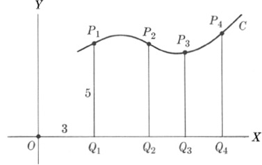
We can understand more readily what Descartes and Fermat accomplished if we examine a somewhat modernized version of their idea. In his general study of methodology, Descartes had decided to solve problems by proceeding from the simple to the complex. Now the simplest figure in geometry is the straight line, and so Descartes sought to analyze curves by working with straight lines. He observed, first of all, that if one introduces (Fig. 12–1) a horizontal line, OX, then the shape of a curve C could be studied by observing how vertical line segments such as Q1P1, Q2P2, Q3P3, . . . changed in length.
Fig. 12–1
The next step was to express this information in arithmetical terms. The position of Q1, for example, could be specified by stating its distance from a fixed point O, called the origin, on the horizontal line. The length Q1P1 could certainly be specified by a number. Thus the position of P1 would be determined by two numbers, the length OQ1 and the length Q1P1. The length OQ1 which is 3 in Fig. 12–1, is called the abscissa of P1, and the length P1Q1, which is 5 in Fig. 12–1, is called the ordinate. The line OX is called the X-axis, and the line OY, which is perpendicular to OX and which shows the direction in which Q1P1 is taken, is called the Y-axis.
Stated in more general terms, Descartes’ and Fermat’s first step was to describe the position of any point P on a curve by two numbers, an abscissa and an ordinate. The first expresses the distance or length from O along the X-axis to the point Q directly below P, and the second denotes the distance or length from Q to P along a line perpendicular to the X-axis or parallel to the Y-axis. The pair of numbers is called the coordinates of P and is written thus: (3, 5).
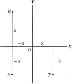
Fig. 12–2.
Plotting points on a rectangular Cartesian coordinate system.
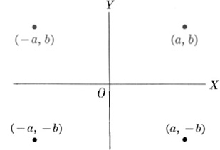
To distinguish points which are reached by proceeding along the X-axis to the right of O from those which are reached by proceeding to the left of O, distances to the left are represented by negative numbers. Thus to arrive at the point R of Fig. 12–2 one proceeds 3 units to the left along the X-axis and 5 units upward in the direction of the Y-axis. The coordinates of R are therefore –3 and 5 and are represented as (– 3, 5). The distinction between upward and downward is also made by using positive and negative numbers, and as a consequence the coordinates of S in Fig. 12–2 are –3 and –4, and the coordinates of T are 3 and –4.
Thus far, then, Descartes and Fermat had a simple scheme for representing the position of any point in the plane by means of numbers, these numbers being distances from two arbitrarily chosen but fixed axes. To each point there corresponds a pair of numbers, and to each pair of numbers a unique point. The system using axes and coordinates to represent points is called a rectangular Cartesian coordinate system.
To represent a curve such as C of Fig. 12–1, one could list the coordinates of the many points on the curve, that is, the coordinates of P1, P2, P3, . . . But such a representation would hardly be convenient, for each curve consists of an infinite number of points. Descartes and Fermat had a better idea. First of all they introduced the letters x and y to stand for the coordinates of any one of the points on the curve. When x and y have specific numerical values, for example, 2 and 3, respectively, then they refer, of course, to a definite point. Otherwise they represent an arbitrary point. The use of x and y here is analogous to using the words “man” and “woman” to represent any man or woman in the United States, whereas John and Mary would describe a particular couple.
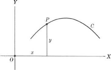
Fig. 12–3
Now, if one looks at the curve C of Fig. 12–3 and observes the abscissas and ordinates of the points on this curve, he notices that as the abscissas increase (as one looks from left to right), the corresponding ordinates at first increase and then decrease. The behavior of the ordinates changes as the abscissas change. Might it not be possible to describe the relationship between these abscissas and ordinates by specifying how large any ordinate is when the corresponding abscissa is named? This description should hold for all points on the curve and apply to that curve and no other. The answer is yes, and the general description turns out to be an algebraic equation involving x and y, the coordinates of an arbitrary point. This statement is a bit vague; let us see, therefore what it means in concrete examples.
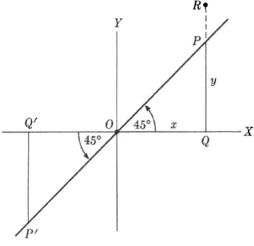
Suppose, first, that the curve happens to be a straight line inclined 45° to the horizontal.* To describe the line algebraically, we introduce a horizontal line which passes through any point O of the given line (Fig. 12–4) and consider this horizontal line as the X-axis of our coordinate system. The Y-axis is then a vertical line through O. Consider any point P on the line. The coordinates of this general point P are the x and y shown in the figure. Now Euclidean geometry tells us that the triangle OQP is an isosceles right triangle. Hence OQ = QP or x = y. Therefore the line OP appears to be characterized by the algebraic equation
because for any point P on the line, the coordinates are such that y = x.
Fig. 12–4.
A straight line on a rectangular Cartesian coordinate system.
Fig. 12–5.
A straight line of slope 3 on a rectangular Cartesian coordinate system.
We should note that this equation also describes points, such as P′, which lie to the left of the vertical axis. Thus, for example, the abscissa of P′ may be –4; now angle Q′OP′ is also 45°, and hence the ordinate of P′ must also be –4. Since abscissa and ordinate are equal, x = y also holds for P′. Then the all-important fact about the line P′P is that it may be described algebraically by the equation y = x. In other words, we may say that the coordinates of any point on the line satisfy the equation y = x. On the other hand, points not on that line, such as R, will have ordinates unequal to the abscissas because, while R has the same abscissa as P, the ordinate of R is larger than the ordinate of P, and hence for R, y does not equal x.
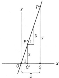
Let us consider a second example. One may describe the line of Fig. 12–4 by saying that it rises one unit for each unit of horizontal distance or, in the customary expression, that it has slope 1. We now consider a line which rises more steeply, for example, one which rises 3 units for each horizontal distance of 1 unit (Fig. 12–5). Again let P be any point on the line. The coordinates of this general point P are then (x, y). Then from the similar triangles OQ′P′ and OQP we may argue that
![]()
Hence
is the equation of the line.
The nature of equations such as y = x and y = 3x requires some attention. In elementary algebra we also treat equations, for example, x2 – 5x + 6 = 0 or 2x + 3 = 7. In these latter equations, however, x represents some definite but unknown quantity and our aim is to find the value or values of x. On the other hand, when we represent a curve by an equation such as y = 3x, we are not seeking to determine unknowns. In fact, x and y are not unknown. They represent the coordinates of any point on the line. Thus x = 3 and y = 9 are one pair of values satisfying the equation; x = 4 and y = 12 constitute another such pair; there are millions of others. The end product of the process of finding the equation of a curve is then an equation involving x and y which states the relationship between x and y peculiar to all points on the curve. Of course, if one wishes to find the coordinates of a particular point on the curve, he can, provided he knows the abscissa of the point, substitute this number for x in the equation and now solve for the ordinate. Thus, if the given line has the equation y = 3x and we wish to determine the ordinate of the point whose abscissa is ![]() , we substitute
, we substitute ![]() for x and immediately find that the ordinate of this point is
for x and immediately find that the ordinate of this point is ![]() .
.
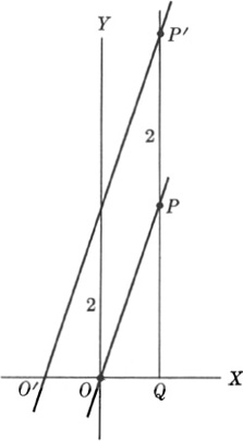
Let us consider next another example which will enlarge our understanding of these new equations. Suppose we are given two straight lines as shown in Fig. 12–6. The line OP is the one we have just discussed and its equation is y = 3x. The line O′P′ is supposed to be parallel to OP and 2 units above it; that is, PP′ is 2. What is the equation of the line O′P′?
To answer this question, we again seek the relation between x and y which holds for any point on this line. Now P and P′ have the same x-value or abscissa, namely OQ. But the ordinate of P′ is larger than that of P by the amount PP′. The distance PP′ is given to be 2. Since the two lines are parallel, the vertical distance between a point on OP and a point on O′P′ will always be 2. Hence, whereas the ordinate of each point on the line OP is always 3 times the abscissa, the ordinate of each point on O′P′ will be 3 times the abscissa plus 2. That is, the equation of O′P′ is
We should note that although the straight line O′P′ is identical except for position with the straight line OP, its equation is different. The difference results from the fact that OP passes through the origin O of the system of coordinates, whereas O′P′ does not. Hence the very same curve may be represented by a different equation if its position with respect to the coordinate axes is changed.
Why do we bother with different equations for the same curve? If a straight line having a slope of 3 can always be placed on a coordinate system so that its equation is y = 3x, why do we have to consider the more complicated form y = 3x + 2? The answer is that if one wishes to work with two straight lines simultaneously and keep these lines in the same relative positions which they may happen to have in some physical application, one cannot assign to them an identical position on the set of axes.
Fig. 12–6.
Two parallel lines of slope 3 on a rectangular Cartesian coordinate system.
Fig. 12–7.
A line with negative slope.
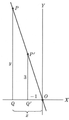
While we are discussing equations of straight lines, we wish to note one more case which will be of interest later. Let us compare the line OP of Fig. 12–7 with the line OP of Fig. 12–5. The line in Fig. 12–7 may be said to “fall” as one views it from left to right, whereas that in Fig. 12–5 rises. Alternatively, we may say that the ordinates in Fig. 12–7 decrease as the abscissas increase. What is the equation of the line OP of Fig. 12–7? Suppose that the coordinates of some point P′ on the line are (– 1, 3). The point P is an arbitrary point of the line OP, so let us denote its coordinates by x and y. Again we have the similar triangles OQP and OQ′P′. Insofar as mere lengths, without regard to sign, are concerned, we can say that
![]()
However, we know that for the line OP, the ordinate of any point is always opposite in sign to the abscissa of that point. That is, when y is a positive number, x is a negative one and conversely. Hence, in the present case, not y = 3x, but
is the equation of the line OP. Thus the fact that OP falls to the right is reflected in the negative sign of the coefficient of x. To distinguish, with respect to slope, lines which fall to the right from those which rise to the right, we say that the former have negative slope. Thus the slope of OP is –3.
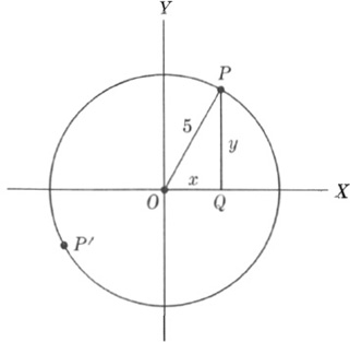
To illustrate Descartes’ and Fermat’s idea once more we shall seek the equation of a circle. Suppose that we choose our axes so that the origin is at the center of the circle (Fig. 12–8). Now the circle is defined to be the collection of all points which are at the same distance from one point, called the center. Let us assume that this distance is 5 units. (The quantity 5 is, of course, the length of the radius.) Since each point on the circle is described by a pair of coordinates, the problem of finding the algebraic equation of this circle can be solved by answering the following question. What property or relationship do the coordinates of points on the circle possess which distinguishes them from those of other points? If we consider a typical point P on the circle and let x and y represent its two coordinates, then we see that the lengths x, y, and 5 form a right triangle. According to the Pythagorean theorem of Euclidean geometry, the square of OP must equal the square of OQ plus the square of QP; hence
This same statement also holds for points on the circle such as P′, for even though the coordinates of P′ are negative, their squares are positive and so satisfy equation (5). Equation (5) is the algebraic representation of the circle. It says in words that the square of the abscissa of any point on the curve plus the square of the ordinate equals the square of the radius.
Fig. 12–8.
A circle on a rectangular Cartesian coordinate system.
To decide algebraically whether any point belongs to the circle represented by equation (5), we have to test whether the coordinates of the point satisfy the equation. Thus the point whose abscissa is 3 and whose ordinate is 4 belongs to the circle under discussion because, substituting 3 for x and 4 for y in equation (5), we see that the resulting left side equals the right side, that is, 32 + 42 = 52. As another example, let us consider the point whose abscissa is 2 and whose ordinate is ![]() . Again, substituting 2 for x and
. Again, substituting 2 for x and ![]() for y in equation (5), we find that
for y in equation (5), we find that
![]()
because the square of ![]() is 21. Thus the point whose coordinates are (2,
is 21. Thus the point whose coordinates are (2, ![]() ) lies on the circle.
) lies on the circle.
1. What is meant by the coordinates of a point?
2. State in your own words what the equation of a curve is.
3. Find the equation of the straight line which
a) rises 2 units for each horizontal distance of one unit and passes through the origin of the coordinate system chosen;
b) makes an angle of 30° with the X-axis and passes through the origin [Suggestion: ![]() .];
.];
c) falls 4 units for each unit of horizontal distance traversed and passes through the origin;
d) passes through the origin and has slope 4;
e) passes through the origin and has slope –4.
4. Find the coordinates of one point which lies on the curve whose equation is
a) x + 2y = 71;
b) x2 + y2 = 36.
5. Does the point whose coordinates are (– 3, 5) lie on the curve whose equation is x2 + 2y2 = 59?
6. Determine whether the point whose coordinates are (3, –2) lies on the curve whose equation is x2 + y2 = 4x + 1.
7. Describe the curve whose equation is
a) y = 3x + 7,
b) x2 + y2 = 49,
c) x2 + y2 = 20,
d) x + 2y = 6,
e) y2 = 20 – x2.
8. Would latitude and longitude serve as a coordinate system for points on the surface of the earth?
9. Can a curve have more than one equation? If so, how is this possible?
10. Can you say anything about the slope of the line whose equation is y = mx + 2?
11. What are the coordinates of the point of intersection of the line y = 3x + 7 and the Y-axis?
12. What are the coordinates of the point of intersection of the line y = 3x + b and the Y-axis?
13. What is the slope of the line whose equation is y = mx + b, and what are the coordinates of the point where the line cuts the Y-axis?
14. The equation of a circle with center at the origin and radius 1 is
The equation of a circle with center at the origin and radius 2 is
If we subtract equation (a) from equation (b), we obtain the result 0 = 3. What is wrong?
Fig. 12–9.
A parabola on a rectangular Cartesian coordinate system.
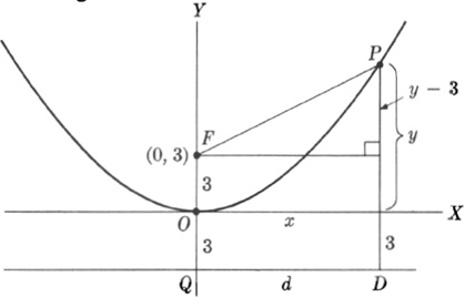
The curve most widely used, next to the straight line and circle, is the parabola. Let us see how this curve is represented algebraically. Recalling the definition of the parabola given in Chapter 6, we start with a fixed line d, called the directrix, and a fixed point F (Fig. 12–9), called the focus. We now consider all points each of which is equidistant from d and F. This set of points is called a parabola. Thus if P is a typical point on the parabola determined by d and F, then the distance from P to F must equal the distance from P to d, that is
To obtain the equation of this curve, we first introduce a set of coordinate axes. We know from the discussion of the straight line that the same curve may have different equations, depending upon how one chooses the axes in relation to the curve. Mathematicians have learned by experience that a simple equation results if the axes are chosen in the following way (see Fig. 12–9). Let the Y-axis be the line through F and perpendicular to d. The X-axis, which is, of course, perpendicular to the Y-axis, is drawn halfway between F and d.
Since the point F and the line d are fixed, the distance from F to d, namely FQ, is fixed. Let us suppose that this distance is 6 units. Then the distance OF is 3 units, and the distance OQ is also 3 units because the X-axis is halfway between F and d. Then the coordinates of F are (0, 3). We now wish to express equation (6) in algebraic terms. Let P be any point on the parabola. Then its coordinates are (x, y). We see that PF is the hypotenuse of a right triangle whose sides are x and y – 3. Hence, by the Pythagorean theorem,
![]()
The perpendicular distance from P to d is y + 3. Thus, in algebraic terms, equation (6) states that
Equation (7) is the equation of the parabola.
Next we shall perform some algebraic manipulations to simplify the form of this equation. We begin by squaring both sides of the equation, an operation which amounts to multiplying equals by equals. Squaring the left side removes the radical, and squaring the right side yields y2 + 6y + 9. Hence we now have
x2 + (y – 3)2 = y2 + 6y + 9.
We now write out in full the square called for on the left side and obtain
x2 + y2 – 6y + 9 = y2 + 6y + 9.
Subtracting y2 and 9 from both sides yields
x2 – 6y = 6y.
We add 6y to both sides and obtain x2 = 12y or, as we prefer to write it,
12y = x2.
Dividing both sides by 12, we obtain
This equation is much simpler than (7) and yet expresses the same fact.
We might note incidentally that the number 12 in the denominator is twice the distance from F to d. Had we called this distance a, the resulting equation would have read
In Fig. 12–9 we drew a curve which resembles a parabola, but we did not know at the time its position in relation to the axes we chose. To obtain a
Fig. 12–10
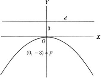
Fig. 12–11.
A parabola with focus below the directrix.
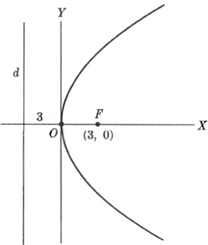
Fig. 12–12.
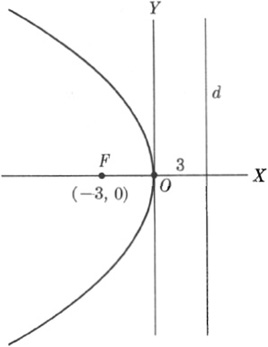
A parabola with focus to the right of the directrix.
rough idea of this position, let us substitute into equation (8) any positive value of x, say 5. Then ![]() . This tells us that (5,
. This tells us that (5, ![]() ) is a point on the curve (Fig. 12–10). But if we substitute –5 for x, we obtain the same result for y. Thus (– 5,
) is a point on the curve (Fig. 12–10). But if we substitute –5 for x, we obtain the same result for y. Thus (– 5, ![]() ) is another point on the curve. These two points are symmetrically situated with respect to the Y-axis. Moreover, no matter which abscissa and ordinate we calculate, the negative of that abscissa will always yield the same ordinate because the abscissa has to be squared. This means that to each point on the curve to the right of the Y-axis there corresponds a point symmetrically situated to the left of the Y-axis. Hence, once we have determined the shape of the curve to the right of the Y-axis, we automatically know what the curve looks like to the left.
) is another point on the curve. These two points are symmetrically situated with respect to the Y-axis. Moreover, no matter which abscissa and ordinate we calculate, the negative of that abscissa will always yield the same ordinate because the abscissa has to be squared. This means that to each point on the curve to the right of the Y-axis there corresponds a point symmetrically situated to the left of the Y-axis. Hence, once we have determined the shape of the curve to the right of the Y-axis, we automatically know what the curve looks like to the left.
If we are interested only in the shape of the curve, it is now sufficient to observe that as x increases from zero to any value, x2 increases, and x2/12 also increases. This means that the points on the curve move out and up from the origin. Of course, there are many curves that meet this description. To obtain a more precise picture of the curve we need to calculate a few sets of coordinates. Thus, when x = 3, ![]() , so that (3,
, so that (3, ![]() ) are the coordinates of a point on the curve. We should note, too, that the curve lies entirely above the X-axis except, of course, for the point at the origin, because for every value of x, y is zero or positive.
) are the coordinates of a point on the curve. We should note, too, that the curve lies entirely above the X-axis except, of course, for the point at the origin, because for every value of x, y is zero or positive.
In work involving parabolas and their equations it is sometimes convenient to consider one whose focus lies below the directrix. If we now choose the axes as shown in Fig. 12–11, what is the equation of the parabola? We could, of course, obtain the answer by going through steps analogous to those contained in equations (6) through (8). However, there is no need to do so since Figs. 12–9 and 12–11 differ only in the sign of the y-values: whereas the y-values in the former are positive, the y-values in the latter must be negative. Hence the equation of the parabola in Fig. 12–11 is
Let us consider Fig. 12–11, but suppose now that distances downward on the Y-axis are chosen to be positive. How does this change affect the equation of the parabola? The suggested situation does not really differ from that shown in Fig. 12–9. If we imagine this whole figure rotated about the X-axis through 180°, that is through half a rotation, we obtain the situation we have just proposed. Since the position of the curve in relation to the X- and Y-axes is exactly the same in Fig. 12–11 as in Fig. 12–9, the parabola has the equation
Let us consider one more variation. Suppose that directrix and focus happen to lie as in Fig. 12–12. We choose the X- and Y-axes as shown, with the Y-axis halfway between focus and directrix. The upward direction on the Y-axis is positive. What is the equation of the parabola determined by this choice of focus, directrix, and axes? To answer this question we have but to compare Figs. 12–9 and 12–12. The X-axis in Fig. 12–9 plays the role of the Y-axis in Fig. 12–12, and the Y-axis in Fig. 12–9 plays the role of the X-axis in Fig. 12–12; in other words, the roles of abscissa and ordinate are exchanged. Hence the equation of the parabola in Fig. 12–12 is
These last few equations illustrate some of the various forms which the equation of the parabola can take. Which of these one should use is a matter of convenience in application, as we shall see in later chapters.
1. Determine the shapes of the following parabolas by choosing a number of values of x, calculating the corresponding values of y, and plotting the points whose coordinates are thereby determined.
a) y = 3x2
b) ![]()
c) y = –3x2
d) x = 2y2
e) ![]()
f) 2x = y2
Fig. 12–13
Fig. 12–14
Fig. 12–15
2. Compare the curves of Exercises 1(a) and 1(b).
3. For the parabola shown in Fig. 12–13, the distance from focus to directrix is 6. What is the equation of the parabola?
4. If the equation of a parabola is ![]() , what are the coordinates of the focus? Describe the position of the directrix.
, what are the coordinates of the focus? Describe the position of the directrix.
5. The following exercises specify the position of focus and directrix of a parabola in relation to a coordinate system. Find the equation of the parabola.
a) Focus (0, 4); directrix parallel to, and 4 units below, the X-axis.
b) Focus (0, 6); directrix parallel to, and 6 units below, the X-axis.
c) Focus (0, –5); directrix parallel to, and 5 units above, the X-axis.
d) Focus (4, 0); directrix parallel to, and 4 units to the left of, the Y-axis.
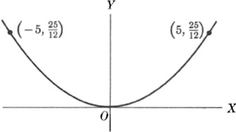
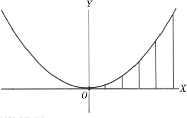
6. Suppose that the designer of a bridge has decided to use the parabolic cable y = x2 for the range x = –5 to x = 5 (Fig. 12–14). The roadbed of the bridge is to be the X-axis. Compute the lengths of straight wire needed to suspend the roadbed from the cable at x = 1, 2, 3, 4, and 5.
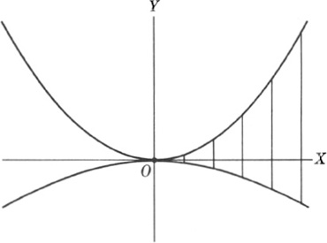
7. Suppose that the designer of a bridge has decided to use the parabolic cable y = x2 for the range x = –5 to x = 5 (Fig. 12–15). The roadbed is to have the shape ![]() . Compute the length of straight wire needed to suspend the roadbed from the cable at x = 1, 2, 3, 4, and 5.
. Compute the length of straight wire needed to suspend the roadbed from the cable at x = 1, 2, 3, 4, and 5.
The great merit of the idea conceived by Fermat and Descartes is that it permits us to represent a curve algebraically and, as we shall see later, learn much about the curve by working with the equation. But another value of their idea, hardly secondary in importance, is that any equation in x and y determines a curve. Hence by merely writing down any equation we please and by finding out what curve belongs to the equation we can discover many new curves. Although we shall not, at this time, make any sensational discoveries, let us see how the process of determining the curve of an equation can be carried out.
Suppose we consider the equation
and try to determine the curve which has this equation. A direct method would be to calculate coordinates of points on the curve and then plot these points. Thus, when x = 2, y = –8, and so (2, –8) are the coordinates of a point on the curve. By calculating many such sets of coordinates and by plotting the corresponding points one can determine the shape of the curve. However, one often learns more by applying a little algebra.
If equation (13) had been y = x2, we would know at once by comparing with equation (9) that it is a parabola with distance from focus to directrix equal to ![]() . Let us see whether a little algebraic juggling with equation (13) might bring it into a form which will permit us to identify the curve. By adding 9 to both sides of equation (13) we obtain
. Let us see whether a little algebraic juggling with equation (13) might bring it into a form which will permit us to identify the curve. By adding 9 to both sides of equation (13) we obtain
y + 9 = x2 – 6x + 9.
Now our knowledge of algebra tells us that the right side is (x – 3)2. Hence we have
Suppose we introduce new letters x′ and y′ such that
Then substitution in equation (14) yields
Fig. 12–16
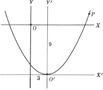
The curve corresponding to this equation is the parabola shown in Fig. 12–16, where it is graphed with respect to the X′- and Y′-axes. Of course, we wish to find the curve corresponding to equation (13), not that described by (16). However, equations (15) provide the necessary connection. The equation x′ = x – 3, or x = 3 + x′, tells us that the abscissas x of points belonging to (13) should be 3 more than the abscissas x′ of points belonging to (16). How can we increase by 3 the abscissas of each point in Fig. 12–16? The answer is simple. We draw a new Y-axis 3 units to the left of the Y′-axis. Then the x-value of a typical point such as P is 3 units more than its x′-value. We now use the second equation in (15), that is, y′ = y + 9, or y = y′ – 9. This equation says that the y-values of points should be 9 units less than the y′-values. How can we reduce by 9 the ordinates of the curve in Fig. 12–16? We have already indicated the essential trick. We introduce a new X-axis 9 units above the X′-axis. Now the y-value of P is 9 units less than the y′-value. Hence with respect to the X- and Y-axes, the points of the parabola y′ = x′2 have the correct x- and y-values called for by equation (13). Since we did not change the curve in any way by introducing the X- and Y-axes, but merely changed the axes, the curve of equation (13) is a parabola placed with respect to the X- and Y-axes as shown in Fig. 12–16.
We were a bit lucky in analyzing equation (13) because the introduction of new coordinates in equation (15) reduced equation (13) to equation (16) whose curve we already knew. If this change to a familiar form is not possible, then the initial equation may indeed represent some new curve, and by analyzing the equation we might get to know the properties of this new curve. The results of such studies would be a further addition to the stock of knowledge about equations and their corresponding curves, a type of knowledge which the professional mathematician builds up for his work just as a writer may build up a bigger and bigger vocabulary. Thus through the notion of equation and curve, Fermat and Descartes opened up to mathematicians a vast variety of new curves.
1. For equation (13) of the text calculate the coordinates of a number of points on the curve and plot the points. Then sketch in the curve. Does your graph look like the one in Fig. 12–16?
2. Determine the curve whose equation is y = x2 – 10x.
3. Determine the curve whose equation is y = –x2 + 6x. [Suggestion: Note that the given equation is the same as –y = x2 – 6x and use the results obtained for equation (13) of the text.]
4. Sketch the curve whose equation is y = –x2 + 6x by finding and plotting the coordinates of a number of points on the curve.
5. Knowing the curve which corresponds to y = x2 – 6x, can you determine the curve which corresponds to y = x2 – 6x + 9?
6. What does one mean by the statement that a curve can be associated with any equation in x and y?
7. Sketch the curves whose equations are given below.
a) y = x3
b) y = x3 + 9
c) ![]()
Does the sketch of part (c) suggest one of the conic sections?
Another very widely used curve is the ellipse. Let us review the definition given in Chapter 6. We start with two fixed points, F and F′, called foci, and a constant quantity which is greater than the distance FF′. We now consider all points, the sum of whose distances from F and F′ is the constant quantity. This set of points is called an ellipse. To be more concrete, suppose that the distance FF′ is 6 and that the constant quantity is 10. If P is a point such that PF + PF′ is 10, then P is a point on the ellipse.
Fig. 12–17.
An ellipse on a rectangular Cartesian coordinate system.
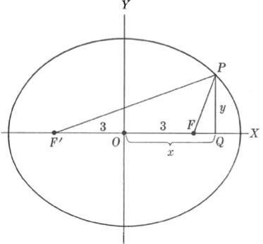
From the standpoint of coordinate geometry, the first thing of interest about the ellipse is its equation. Let us see whether we can find it. As in the case of the parabola, experience has taught mathematicians that the resulting equation will be simplest if the line FF′ (Fig. 12–17) is chosen as the X-axis and the Y-axis is chosen to be the line perpendicular to the X-axis and halfway between F and F′. Let us consider the ellipse for which the length FF′ is 6 units. Then the coordinates of F are (3, 0) and those of F′ are (– 3, 0). Now let P be any point on the curve and let us denote its coordinates by (x, y). If the constant quantity which determines the ellipse is 10, then the condition which any point P on the ellipse satisfies is
We wish to express this condition algebraically. The procedure is straight-forward. The distance PF is the hypotenuse of the right triangle PQF whose arms are x – 3 and y. Hence ![]() . The distance PF′ is the hypotenuse of the right triangle PQF′ whose arms are x + 3 and y. Hence
. The distance PF′ is the hypotenuse of the right triangle PQF′ whose arms are x + 3 and y. Hence ![]() . Thus equation (17) amounts to
. Thus equation (17) amounts to
We are now in the same position that we were in when we arrived at equation (7) for the parabola. We could maintain that (18) is the equation of the ellipse, for it is indeed the condition which the coordinates (x, y) of any point on the ellipse satisfy. However, as for the parabola, a little algebra applied to (18) will simplify the equation. We shall not carry out the algebraic steps explicitly because they are uninteresting, and it is not important for us to acquire great facility in algebra. The result is
We know what an ellipse looks like: But we do not know how our ellipse lies in relation to the axes chosen in Fig. 12–17. An analysis of equation (19) will supply the answer. First of all let us note that if (a, b) should happen to be the coordinates of a point which satisfy equation (19), that is, if
Fig. 12-18
then the sets of coordinates (–a, b), (a, –b), and (–a, –b) will also satisfy the equation, because the substitution of any one of these latter three pairs of coordinates will yield the same equation as (20). Figure 12–18 shows where the various points (a, b), (–a, b), (a, –b), and (–a, –b) lie in relation to the axes. We see, for example, that (a, b) and (–a, b) are symmetrically placed with respect to the Y-axis. What we have learned so far is that if the ellipse contains a point (a, b) which lies in the first quadrant, it contains the point (–a, b) which is symmetrically situated with respect to the Y-axis; it contains the point (a, –b) which is symmetrically situated with respect to the X-axis; and it contains the point (–a, –b) which is symmetric to (–a, b) with respect to the X-axis. Hence, if we can determine which points lie on the ellipse in the first quadrant, we can, by symmetry, decide what the ellipse looks like in the other three quadrants.
The shape of the ellipse in the first quadrant is easily determined. We have but to calculate the coordinates of a number of points in the first quadrant and plot the points carefully with respect to the coordinate axes. By symmetry we obtain the shape of the curve in the other three quadrants. The final graph is that shown in Fig. 12–17.
We could investigate the equations of other curves and the curves corresponding to other equations. But what we have done should make the primary idea clear. To each curve there corresponds an equation which describes that curve. The equation depends upon how we choose the axes, but once this choice is made, the equation is unique. Conversely, given an equation involving x and y, we can find the curve which this equation describes, namely the collection of points whose coordinates satisfy the equation.
1. For equation (19) of the text, calculate the coordinates of the points whose abscissas are 0, 1, 2, 3, 4, 5. Plot the points.
2. Sketch the ellipse whose equation is 9x2 + 6y2 = 144.
3. Calculate the length of the X-axis which is contained within the ellipse represented by equation (19). Does this length have any relation to any of the quantities which determine the ellipse? This length is called the major axis of the ellipse.
4. Suppose that the constant quantity which defines an ellipse, 10 in the example discussed in the text, is retained, but the distance between the foci F and F′ is 0. What changes must one make in equation (18)? Can you now simplify the equation and recognize the curve that it represents?
5. Kepler’s first law of planetary motion says that the path of each planet is an ellipse with the sun at one focus. Let us suppose that equation (19) of the text is the equation of some planet’s path and that the sun is at F. What is the planet’s distance from the sun when it crosses the positive X-axis and what is the distance when it crosses the negative X-axis?
The mathematician has but to get hold of an idea, and he will develop it for all that it is worth. It had already occurred to Descartes that the idea of equations for curves might be extended to finding equations for surfaces. This possibility was soon explored.
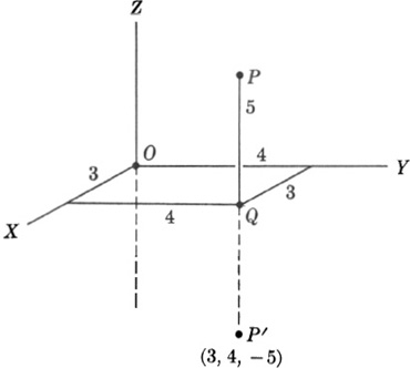
A curve can lie in one plane, but surfaces such as a sphere or the ellipsoid (of which the surface of the earth and the surface of a football are examples), do not lie in one plane. They exist in three-dimensional space. To pursue the idea of finding equations for surfaces, we must first introduce coordinates for points in space. This is readily done. One introduces three mutually perpendicular lines (Fig. 12–19) as axes instead of the two lines used for points in the plane. These are called the coordinate axes. The X- and Y-axes determine a plane called the XY-plane. Similarly, the X- and Z-axes determine the XZ-plane, and the Y- and Z-axes define the YZ-plane.
The location of a point P in space is described by three numbers. For example, the point P of Fig. 12–19 is described by (3, 4, 5). The number 5
Fig. 12–19.
A three-dimensional rectangular Cartesian coordinate system
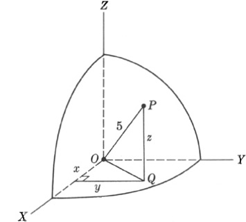
Fig. 12–20.
A sphere on a three-dimensional rectangular Cartesian coordinate system.
describes the perpendicular distance of P above the XY-plane, while 3 and 4 are the x- and y-coordinates of Q, the foot of the perpendicular from P to this plane. Alternatively one can say that if one proceeds a distance of 3 units along the X-axis, then a distance of 4 units along a parallel to the Y-axis, and finally travels upward a distance of 5 units along the perpendicular to the XY-plane, he will arrive at the point P. To represent all points in space, we must, as in the two-dimensional system, use negative numbers also. Thus points below the XY-plane have negative third coordinates.
Let us now consider the problem of finding the equation of a surface. We shall use the sphere as an example. A surface, like a curve, has some defining property which states just which points belong to it. By definition, the sphere is the set of all points in space at a given distance, the radius, from a fixed point called the center. To be concrete let us suppose that all points of our sphere are 5 units from the center and that the sphere is located so that its center is at the origin of our three-dimensional coordinate system (Fig. 12–20). The general point on a surface is represented by three letters, x, y, z. Thus the coordinates of the general point P are (x, y, z). Let us now express algebraically the fact that the distance of any point (x, y, z) on the sphere is 5 units from the origin. The lengths x, y, and z are shown in Fig. 12–20. Now x and y are the arms of a right triangle (lying in the XY-plane) whose hypotenuse is OQ. Then by the Pythagorean theorem,
Further OQ and z are the arms of the right triangle OQP, whose hypotenuse is OP or 5 units. Hence
But OQ2 has the value given by equation (21). If we substitute this value in equation (22), we obtain
This is the equation of a sphere in the sense that the left side equals the right side when and only when the coordinates of a point on the sphere are substituted for x, y, and z.
We could readily obtain the equations of a few other surfaces, such as plane, paraboloid, and ellipsoid. But we shall not do so because we shall not utilize three-dimensional coordinate geometry and the procedure involved is a more or less apparent extension of a familiar concept.
1. Plot the points whose coordinates are given below.
a) (1, 2, 3)
b) (1, 2, -3)
c) (-1, 2, 3)
d) (1, -2, 3)
2. What geometrical figure does an equation in x, y, and z represent?
3. Describe the surface whose equation is x2 + y2 + z2 = 49.
4. We know that an equation such as x + y = 5 represents a straight line. What does the equation x + y + z = 5 represent?
Our experience is limited to figures lying in a plane and in space. But our intellects are not. The idea of a four-dimensional world and of figures in it had tantalized mathematicians such as Pascal at a time when coordinate geometry was still being fashioned. During the next 200 years the subject was mentioned occasionally, but it was not taken seriously until some startling developments (which we shall consider in Chapter 20) caused a number of mathematicians, notably Bernhard Riemann, to investigate it. Four-dimensional geometry proved to be more than a speculation, for some of the deepest developments in modern science, notably the theory of relativity, use this concept. Let us see how coordinate geometry can be employed to portray a four-dimensional world.
We have seen that the equation of a circle of radius 5 in a two-dimensional coordinate system is
and we have just seen that the equation of a sphere of radius 5 in a three-dimensional coordinate system is
Even idle speculation would suggest that we at least write down the equation
and consider what meaning it might have. It would seem reasonable to interpret x, y, z, and w as the coordinates of a point in four-dimensional space and, by analogy with equations (24) and (25), to interpret equation (26) as the equation of a hypersphere in four-dimensional space. This is exactly what mathematics does. However, mathematics does not suppose that there is anywhere a real four-dimensional space in which four mutually perpendicular axes can be set up. Nor do mathematicians claim that they, wise and farsighted as they think they are, can visualize figures in a four-dimensional space. It follows that no one else can either.
Four-dimensional geometry is entirely a creation of the mind; it is a geometry without pictures. One speaks of the coordinates (x, y, z, w) as representing a point, and one uses the term hypersphere as though it were a real geometrical figure corresponding to equation (26), but these geometrical terms are merely a convenience and a carry-over from two- and three-dimensional geometry. The words are suggestive but not descriptive of actual figures.
Suppose it is agreed then that four-dimensional geometry is indeed a mental creation. Is it of any value? There is excellent reason to study this “geometry”, and there is excellent use for it. We can understand these facts better if we backtrack a bit. Consider the equation x2 + y2 = 25. It represents, as we know, a circle. But where is this curve that knows no end, this “arc unbroken”, the cherished figure of the Greeks? Every geometrical fact we know or can establish about the geometrical circle has its algebraic equivalent and can be derived algebraically from the equation of the circle. Hence the equations of the circle and of other curves in plane, or two-dimensional, geometry are a complete substitute for their geometrical counterparts, and we could, if we wished to, eliminate geometry altogether. In four-dimensional “geometry” we have only the equations, but we talk about them as though they represented figures in a four-dimensional world. The properties of these figures are completely specified by the equations. What is lacking is the possibility of actually constructing such figures.
So far then we have tried to see what meaning this four-dimensional geometry has. Now we wish to know how it is used. One application is made in studying physical events wherein time plays a role. Consider for example, the motion of a planet. The location of a planet is described by three coordinates x, y, and z. But the instant at which the planet occupies that location is also important. An eclipse of the sun, for example, occurs because planet and sun are in certain positions at the same instant. Hence the full description of the position of a heavenly body requires four coordinates, the fourth being a value of time. The path of a celestial object is described by equations involving four letters, usually x, y, z, and t.
But is there any value to thinking geometrically about equations involving four letters? There is. Let us consider the usual sphere for a moment. Some curves on this sphere, a circle of latitude, for example, lie in one plane, and hence only two-dimensional geometry is needed to visualize some curves which lie on a three-dimensional sphere. Similarly, the path on which a planet moves in the four dimensions of space and time may be a curve which can exist in three-dimensional space. This curve may be part of a “geometrical structure” which lies in four-dimensional space, just as the circle of latitude is part of a sphere and yet the curve can be visualized. This visualization aids the understanding. This same visualization might be possible for the paths of other planets and one can consequently better understand their motions. Yet the proper interrelationship of these several paths can be represented only in four-dimensional space just as the relationship of the circles of latitude to one another can be represented only in three-dimensional space. We see therefore that it is helpful to think in terms of geometrical figures lying in a four-dimensional space.
This brief presentation of four-dimensional geometry may give some further indication of the direction in which scientific thought has been moving with the aid of mathematics. Copernicus asked the world to accept a theory of planetary motions which violated some sense impressions for the sake of a better mathematical account. The utilization of a four-dimensional geometry which has no sensuous or visual content means complete reliance upon the mind.
From the purely mathematical standpoint coordinate geomery offers a brand-new thought, the representation of geometrical figures by equations. It also offers, as Descartes and Fermat had expected, a new mathematical method of deriving properties of figures from equations. For example, the fact that a curve is symmetric with respect to some line is readily seen from the equation, as we observed in the case of parabola and ellipse.
But Descartes’ and Fermat’s union of algebra and geometry means far more than a new mathematical method of working with curves. The forms of all physical objects which are studied for any reason whatsoever are, at least when idealized, curves and surfaces. The fusilage of an airplane, the wings of an airplane, the hull of a boat, and the shape of a projectile are surfaces. The paths of all moving objects, a ball thrown by a child, an electron expelled from an atom, a ship on the ocean, a plane in the air, the planets in the heavens, and the tracks of light, are curves. These surfaces and curves can be represented by equations, and the shapes or motions studied by applying algebra to these equations. In other words, Descartes and Fermat made possible the algebraic representation and the study by algebraic means of the various objects and paths of interest to scientists. In addition, algebra supplies quantitative knowledge. This method of working with curves and surfaces is so basic in science that Descartes and Fermat may very well be called the founders of mathematical physics. Part of Descartes’ greatness and perhaps the largest part of his contribution was his vision of what his method accomplished; he said he had “reduced physics to mathematics.” The investigation of nature which Renaissance Europe had determined to undertake was enormously expedited as we shall soon see. The story of coordinate geometry illustrates how an interest in geometric method became immensely valuable for science and engineering.
1. In what sense does a four-dimensional geometry exist?
2. What geometrical language would be appropriate to describe the figure whose equation is x + y + z + w = 5?
3. Did Descartes and Fermat introduce a new method for working with curves? If so, describe it.
4. Does coordinate geometry replace Euclidean geometry?
1. What is the x-coordinate of any point on the Y-axis?
2. What is the y-coordinate of any point on the X-axis?
3. If two points lie on a line parallel to the Y-axis, what can you say about their x-coordinates?
4. Write the equation of a line whose slope is 4 and which
a) passes through the origin,
b) cuts the Y-axis at the point (0, 2).
5. Write the equation of a line whose slope is –4 and which
a) passes through the origin,
b) cuts the Y-axis at the point (0, 2),
c) cuts the Y-axis at the point (0, –2).
6. Show that the point whose coordinates are (2, ![]() ) lies on the circle
) lies on the circle
x2 + y2 = 25.
7. Sketch the curves whose equations are given below.
a) ![]()
b) y = 8x2
c) ![]()
8. Sketch the curves whose equations are given below.
a) y = x2 + 6x
b) y = –x2 – 6x
c) y = x2 + 6x + 9, by relating the curve to the one is part (a).
9. Plot the graph of 16x2 + 25y2 = 400 in the first quadrant by solving for y and then making a table of values.
10. Plot the entire graph of the equation x2 – y2 = 4. Can you identify the curve?
11. One can regard the quadratic equation x2 – 6x = 0 as a special case of
y = x2 – 6x,
the special nature being that the values of x which satisfy the first equation are those which correspond to y = 0 in the second one. Can you then suggest a graphical method of solving the quadratic equation?
1. The life and work of René Descartes.
2. The life and work of Pierre de Fermat.
3. Four-dimensional geometry.
ABBOTT, E. A.: Flatland, A Romance of Many Dimensions, Dover Publications, Inc., New York, 1952.
DESCARTES, RENÉ: Discourse on Method, Penguin Books Ltd., Harmondsworth, England, 1960 (also many other editions).
DESCARTES, RENÉ: La Géométrie (the original French and an English translation), Dover Publications, Inc., New York, 1954.
HALDANE, ELIZABETH S.: Descartes, His Life and Times, J. Murray, London, 1905.
MANNING, H. A.: The Fourth Dimension Simply Explained, Dover Publications, Inc., New York, 1960.
SAWYER, W. W.: Mathematicians’ Delight, Chap. 9, Penguin Books Ltd., Harmondsworth, England, 1943.
SCOTT, J. F.: The Scientific Work of René Descartes, Taylor and Francis, Ltd., London, 1952.
WHITEHEAD, ALFRED N.: An Introduction to Mathematics, Chaps. 9 and 10, Holt, Rinehart and Winston, Inc., New York, 1939 (also in paperback).
* In coordinate geometry and in higher mathematics, in general, the word “curve” includes straight lines.