designs in educational experimentation
Experiments, quasi-experiments, single-case research and internet-based experiments |
CHAPTER 16 |
Whilst Chapter 15 provided an overview of a particular kind of experiment (the ex post facto experiment), this chapter constitutes a full exploration of key issues in experiments in education, indicating how they might address causality as a main target of much educational research. The chapter addresses:
designs in educational experimentation
true experimental designs
a quasi-experimental design: the non-equivalent control group design
single-case research: ABAB design
procedures in conducting experimental research
threats to internal and external validity in experiments
the timing of the pre-test and the post-test
examples from educational research
the design experiment
internet-based experiments
The intention here is not only to introduce different forms of experiment but to ensure that researchers are aware of the key issues to be addressed in their planning and conduct, and what might or might not legitimately be inferred from their results.
The issue of causality and, hence, predictability has exercised the minds of researchers considerably (Smith, 1991: 177; Morrison, 2009). One response has been in the operation of control, and it finds its apotheosis in the experimental design. If rival causes or explanations can be eliminated from a study then clear causality can be established; the model can explain outcomes. Smith (1991: 177) and Morrison (2009) claim the high ground for the experimental approach, arguing that it is an important method that directly concerns itself with causality; this, clearly is contestable, as we make clear in Part 3 of the book.
In Chapter 15, we described ex post facto research as experimentation in reverse in that ex post facto studies start with groups that are already different with regard to certain characteristics and then proceed to search, in retrospect, for the factors that brought about those differences. We then went on to cite Kerlinger’s (1970: 22) description of the experimental researcher’s approach: ‘If x, then y; if frustration, then aggression ... the researcher uses some method to measure x and then observes y to see if concomitant variation occurs.’
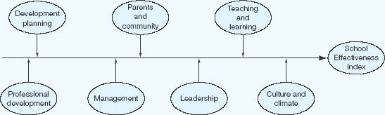
The essential feature of experimental research is that investigators deliberately control and manipulate the conditions which determine the events in which they are interested, introduce an intervention and measure the difference that it makes. An experiment involves making a change in the value of one variable – called the independent variable – and observing the effect of that change on another variable – called the dependent variable. Using a fixed design, experimental research can be confirmatory, seeking to support or not to support a null hypothesis, or exploratory, discovering the effects of certain variables. An independent variable is the input variable, whereas the dependent variable is the outcome variable – the result; for example Kgaile and Morrison (2006) indicate seven independent variables that have an effect on the result (the effectiveness of the school), as shown in Figure 16.1.
In an experiment the post-test measures the dependent variable, and the independent variables are isolated and controlled carefully.
Imagine that we have been transported to a laboratory to investigate the properties of a new wonder fertilizer that farmers could use on their cereal crops, let us say wheat (Morrison, 1993: 44-5). The scientist would take the bag of wheat seed and randomly split it into two equal parts. One part would be grown under normal existing conditions – controlled and measured amounts of soil, warmth, water and light and no other factors. This would be called the control group. The other part would be grown under the same conditions – the same controlled and measured amounts of soil, warmth, water and light as the control group, but, additionally, the new wonder fertilizer. Then, four months later, the two groups are examined and their growth measured. The control group has grown half a metre and each ear of wheat is in place but the seeds are small. The experimental group, by contrast, has grown half a metre as well but has significantly more seeds on each ear, the seeds are larger, fuller and more robust.
The scientist concludes that, because both groups came into contact with nothing other than measured amounts of soil, warmth, water and light, then it could not have been anything else but the new wonder fertilizer that caused the experimental group to flourish so well. The key factors in the experiment were:
the random allocation of the whole bag of wheat into two matched groups (the control and the experimental group), involving the initial measurement of the size of the wheat to ensure that it was the same for both groups (i.e. the pre-test);
the identification and isolation of key variables (soil, warmth, water and light);
the control of the key variables (the same amounts to each group);
the exclusion of any other variables;
the giving of the special treatment (the intervention) to the experimental group (i.e. manipulating the independent variable) whilst holding every other variable constant for the two groups;
ensuring that the two groups are entirely separate throughout the experiment (non-contamination);
the final measurement of yield and growth to compare the control and experimental groups and to look at differences from the pre-test results (the post-test);
the comparison of one group with another;
the stage of generalization – that this new wonder fertilizer improves yield and growth under a given set of conditions.
Of true experiments Morrison writes:
Randomization is a key, critical element of the ‘true’ experiment; random sampling and random allocation to either a control or experimental group is a key way of allowing for the very many additional uncontrolled and, hence, unmeasured, variables that may be part of the make-up of the groups in question (c.f. Slavin 2007). It is an attempt to overcome the confounding effects of exogenous and endogenous variables: the ceteris paribus condition (all other things being equal); it assumes that the distribution of these extraneous variables is more or less even and perhaps of little significance. In short it strives to address Holland’s (1986) ‘fundamental problem of causal inference’, which is that a person may not be in both a control group and an experimental group simultaneously.... As Schneider et al. (2007: 16) remark, because random allocation takes into account both observed and unobserved factors, controls on unobserved factors, thereby, are unnecessary.... If students are randomly allocated to control and experimental groups and are equivalent in all respects (by randomization) other than one group being exposed to the intervention and the other not being exposed to the intervention, then, it is argued, the researcher can attribute any different outcomes between the two groups to the effects of the intervention.
(Morrison, 2009: 143-4)
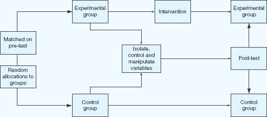
The ‘true’ experiment can be represented diagrammatically as in Figure 16.2.
Schneider et al. (2007: 13) suggest that Holland’s (1986, 2004) ‘fundamental problem of causal inference’ comes into being once one accepts that a causal effect is the difference between what would have happened to a person in an experiment if she had been in the experimental group (receiving the intervention) and if the same person had been in the control group. However, this is impossible to test empirically, as she cannot be in both groups.
FIGURE 16.2 The ’true’ experiment
Note
Average causal effect (A) = (E1-E2) -(C1-C2), where: E1 = post-test for experimental group; E2 = pre-test for experimental group;
C1 = post-test for control group; C2 = pre-test for control group.
Holland (1986: 947) suggests a statistical solution to this through randomization and the measurement of average effects, and Schneider et al. (2007: 13-15) make several suggestions to address Holland’s problem:
Place the same person in the control group, followed by placing her in the experimental groups (which assumes temporal stability (cf. Holland 1986: 948), i.e. the fact that there are two time periods should make no difference to the results, there being a constancy of response regardless of time), assuming or demonstrating that the placement of the person in the first group does not affect the person for long enough to contaminate (affect) the person’s response to being in the second group (cf. Holland 1986: 948) (see the section ‘Repeated measures designs’ below).
Assume that all the participants are identical in every respect (which may be able to be done in the physical sciences but questionably so in the human sciences, even in twin studies: Holland (1986: 947)).
Focus on the average results (Holland, 1986: 948), for example the average scores on the pre-test and post-test, which may be useful unless they mask important differences between subsets of the two samples, e.g. students with a high IQ and students with a low IQ may perform very differently, but this would be lost in an average, in which case stratification into subsample can be adopted.
This model of an experiment, premised on notions of randomization, isolation and control of variables in order to establish causality, may be appropriate for a laboratory, though whether, in fact, a social situation either ever could become the antiseptic, artificial world of the laboratory or should become such a world is both an empirical and a moral question respectively. Indeed, the discussion of the ‘design experiment’ later in this chapter notes that its early advocate (Brown, 1992) had moved away from laboratory experiments to naturalistic settings in order to catch the true interaction of a myriad of variables in the real world. Further, the ethical dilemmas of treating humans as manipulable, controllable and inanimate are considerable (see Chapter 5).
Hage and Meeker (1988: 55) suggest that the experimental approach may be fundamentally flawed in assuming that a single cause produces an effect. Further, it may be that the setting effects are acting causally, rather than the intervention itself, i.e. there is a ‘setting effect’ (where the results are largely a function of their context) (see Maxwell, 2004), for instance in the Milgram studies of obedience and the Stanford prison experiment reported in Chapter 26, and Zim-bardo (2007a, 2007b).
However, despite these concerns about experiments, let us pursue the experimental model further.
Frequently in learning experiments in classroom settings the independent variable is a stimulus of some kind, a new method in arithmetical computation for example, and the dependent variable is a response, the time taken to do 20 sums using the new method. Most empirical studies in educational settings, however, are quasi-experimental rather than experimental. The single most important difference between the quasi-experiment and the true experiment is that in the former case, the researcher undertakes his study with groups that are intact, that is to say, the groups have been constituted by means other than random selection. In this chapter we identify the essential features of true experimental and quasi-experimental designs, our intention being to introduce the reader to the meaning and purpose of control in educational experimentation.
In experiments, researchers can remain relatively aloof from the participants, bringing a degree of objectivity to the research (Robson, 2002: 98). Observer effects can distort the experiment, for example researchers may record inconsistently, or inaccurately, or selectively, or, less consciously, they may be having an effect on the experiment. Further, participant effects might distort the experiment (see the discussion of the Hawthorne effect in Chapter 10); the fact of simply being in an experiment, rather than what the experiment is doing, might be sufficient to alter participants’ behaviour.
In medical experiments these twin concerns are addressed by giving placebos to certain participants, to monitor any changes, and experiments are blind or double-blind. In blind experiments, participants are not told whether they are in a control group or an experimental group, though which they are is known to the researcher. In a double-blind experiment not even the researcher knows whether a participant is in the control or experimental group – that knowledge resides with a third party. These are intended to reduce the subtle effects of participants knowing whether they are in a control or experimental group. In educational research it is easier to conduct a blind experiment rather than a double-blind experiment, and it is even possible not to tell participants that they are in an experiment at all, or to tell them that the experiment is about X when in fact it is about Y, i.e. to ‘put them off the scent’. This form of deception needs to be justified; a common justification is that it enables the experiment to be conducted under more natural conditions, without participants altering their everyday behaviour.
The term ‘control’ has been used in two main senses so far: the random allocation of participants to a control or an experimental group and the isolation and control of variables. Whilst the former is self-evident, the latter has a double meaning which can be explicated a little further, for the control of variables happens at two stages. First, so far the only stage mentioned has been in isolating key independent variables and controlling what happens to these, e.g. so that the same amounts of these are given to both the control group and the experimental group, i.e. the control group and experimental groups are matched in their exposure to these independent variables. This involves giving an identical, measured amount of exposure of both groups to these (whether this can actually be achieved in practice is a moot point, but for the purpose of the discussion here we assume it can). By holding the independent variable constant (giving the same amount to both the control group and the experimental group), it is argued that any changes brought about in the experimental group must be attributable to the intervention, the other variables having been held constant (controlled).
In ex post facto experiments (discussed in Chapter 15), it is not possible to control these variables in advance of the experiment, or during the experiment, the data being already in existence before the experiment has commenced. However, in this case, the controls can be applied at the stage of data analysis, where the researcher can manipulate the independent variables to hold them constant, i.e. to control for the relative effects of these. For an example of this we refer the reader to Chapter 4 on causation, and to Chapter 35 for an indication on how controls can be placed statistically (e.g. partial correlations and crosstabulations).
There are several different kinds of experimental design, for example:
1 The controlled experiment in laboratory conditions (the ‘true’ experiment): two or more groups.
2 The field or quasi-experiment (in the natural setting rather than the laboratory, but where variables are isolated, controlled and manipulated).
3 The natural experiment (in which it is not possible to isolate and control variables).
We consider these in this chapter. The laboratory experiment (the classic true experiment) is conducted in a specially contrived, artificial environment, so that variables can be isolated, controlled and manipulated (as in the example of the wheat seeds above). The field experiment is similar to the laboratory experiment in that variables are isolated, controlled and manipulated, but the setting is the real world rather than the artificially constructed world of the laboratory.
Sometimes it is not possible, desirable or ethical to set up a laboratory or field experiment. For example, let us imagine that we wanted to investigate the trauma effects on people in road traffic accidents. We could not require a participant to run under a bus, or another to stand in the way of a moving lorry, or another to be hit by a motorcycle, and so on. Instead we might examine hospital records to see the trauma effects of victims of bus accidents, lorry accidents and motorcycle accidents, and see which group seems to have sustained the greatest traumas. It may be that the lorry accident victims had the greatest trauma, followed by the motorcycle victims, followed by the bus victims. Now, although it is not possible to say with 100 per cent certainty what caused the trauma, one could make an intelligent guess that those involved in lorry accidents suffer the worst injuries. Here we look at the outcomes and work backwards to examine possible causes. We cannot isolate, control or manipulate variables, but nevertheless we can come to some likely defensible conclusions.
In the outline of research designs that follows we use symbols and conventions from Campbell and Stanley (1963):
X represents the exposure of a group to an experimental variable or event, the effects of which are to be measured.
O refers to the process of observation or measurement.
Xs and Os in a given row are applied to the same persons.
Left to right order indicates temporal sequence.
Xs and Os vertical to one another are simultaneous.
R indicates random assignment to separate treatment groups.
Parallel rows unseparated by dashes represent comparison groups equated by randomization, while those separated by a dashed line represent groups not equated by random assignment.
There are several variants of the ‘true’ experimental design, and we consider many of these below:
the pre-test-post-test control and experimental group design;
the two control groups and one experimental group pretest-post-test design;
the post-test control and experimental group design;
the post-test two experimental groups design;
the pre-test-post-test two treatment design;
the matched pairs design;
the factorial design;
the parametric design;
repeated measures designs.
The laboratory experiment typically has to identify and control a large number of variables, and this may not be possible. Further, the laboratory environment itself can have an effect on the experiment, or it may take some time for a particular intervention to manifest its effects (e.g. a particular reading intervention may have little immediate effect but may have a delayed effect in promoting a liking for reading in adult life, or may have a cumulative effect over time).
A ‘true’ experiment includes several key features:
one or more control groups;
one or more experimental groups;
random allocation to control and experimental groups;
pre-test of the groups to ensure parity;
post-test of the groups to see the effects on the dependent variable;
one or more interventions to the experimental group(s);
isolation, control and manipulation of independent variables;
non-contamination between the control and experimental groups.
If an experiment does not possess all of these features then it is a quasi-experiment: it may look as if it is an experiment (‘quasi’ means ‘as if) but it is not a true experiment, only a variant on it.
An alternative to the laboratory experiment is the quasi-experiment or field experiment, including:
the one-group pre-test-post-test;
the non-equivalent control group design;
the time series design.
We consider these below. Field experiments have less control over experimental conditions or extraneous variables than a laboratory experiment, and, hence, inferring causality is more contestable, but they have the attraction of taking place in a natural setting. Extraneous variables may include, for example:
participant factors (they may differ on important characteristics between the control and experimental groups);
intervention factors (the intervention may not be exactly the same for all participants, varying, for example, in sequence, duration, degree of intervention and assistance, and other practices and contents);
situational factors (the experimental conditions may differ).
These can lead to experimental error, in which the results may not be due to the independent variables in question.
A complete exposition of experimental designs is beyond the scope of this chapter. In the brief outline that follows, we have selected one design from the comprehensive treatment of the subject by Campbell and Stanley (1963) in order to identify the essential features of what they term a ‘true experimental’ and what Ker-linger (1970) refers to as a ‘good’ design. Along with its variants, the chosen design is commonly used in educational experimentation (e.g. Schellenberg, 2004).
The pre-test-post-test control group design can be represented as:
Experimental |
RO1 |
X |
O2 |
Control |
RO3 |
|
O4 |
Kerlinger observes that, in theory, random assignment to E and C conditions controls all possible independent variables. In practice, of course, it is only when enough subjects are included in the experiment that the principle of randomization has a chance to operate as a powerful control. However, the effects of randomization even with a small number of subjects is well illustrated in Box 16.1.
Randomization, then, ensures the greater likelihood of equivalence, that is, the apportioning out between the experimental and control groups of any other factors or characteristics of the subjects which might conceivably affect the experimental variables in which the researcher is interested (cf. Torgerson and Torger-son, 2003a, 2003b). If the groups are made equivalent, then any so-called ‘clouding’ effects should be present in both groups.
So strong is this simple and elegant true experimental design, that all the threats to internal validity identified in Chapter 10 are, according to Campbell and Stanley (1963), controlled in the pre-test-post-test control group design. The causal effect of an intervention can be calculated thus:
Step 1: Subtract the pre-test score from the post-test score for the experimental group to yield score 1.
Step 2: Subtract the pre-test score from the post-test score for the control group to yield score 2.
Step 3: Subtract score 2 from score 1.
Using Campbell and Stanley’s terminology, the effect of the experimental intervention is:
(O2 – ROl) – (O4 – RO3)
If the result is negative then the causal effect was negative.
BOX 16.1 THE EFFECTS OF RANDOMIZATION
Select 20 cards from a pack, ten red and ten black. Shuffle and deal into two ten-card piles. Now count the number of red cards and black cards in either pile and record the results. Repeat the whole sequence many times, recording the results each time.
You will soon convince yourself that the most likely distribution of reds and blacks in a pile is five in each: the next most likely, six red (or black) and four black (or red); and so on. You will be lucky (or unlucky for the purposes of the demonstration!) to achieve one pile of red and the other entirely of black cards. The probability of this happening is 1 in 92,378! On the other hand, the probability of obtaining a ‘mix’ of not more than six of one colour and four of the other is about 82 in 100.
If you now imagine the red cards to stand for the ‘better’ ten children and the black cards for the ‘poorer’ ten children in a class of 20, you will conclude that the operation of the laws of chance alone will almost probably give you close equivalent ‘mixes’ of ‘better’ and ‘poorer’ children in the experimental and control groups.
Source: Adapted from Pilliner, 1973
One problem that has been identified with this particular experimental design is the interaction effect of testing. Good (1963) explains that whereas the various threats to the validity of the experiments listed in Chapter 10 can be thought of as main effects, manifesting themselves in mean differences independently of the presence of other variables, interaction effects, as their name implies, are joint effects and may occur even when no main effects are present. For example, an interaction effect may occur as a result of the pre-test measure sensitizing the subjects to the experimental variable.1 Interaction effects can be controlled for by adding to the pre-test-post-test control group design two more groups that do not experience the pre-test measures. The result is a four-group design, as suggested by Solomon below. Later in the chapter, we describe an educational study which built into a pretest-post-test group design a further control group to take account of the possibility of pre-test sensitization.
Randomization, Smith (1991: 215) explains, produces equivalence over a whole range of variables, whereas matching produces equivalence over only a few named variables. The use of randomized controlled trials (RCTs), a method used in medicine, is a putative way of establishing causality and generalizability (though, in medicine, the sample sizes for some RCTs is necessarily so small – there being limited sufferers from a particular complaint – that randomization is seriously compromised).
A powerful advocacy of RCTs for planning and evaluation is provided by Boruch (1997). Indeed he argues (p. 69) that the problem of poor experimental controls has led to highly questionable claims being made about the success of programmes. Examples of the use of RCTs can be seen in Maynard and Chalmers (1997).
The randomized controlled trial is the ‘gold standard’ of many educational researchers, as it purports to establish controllability, causality and generalizability (Curriculum, Evaluation and Management Centre, 2000; Coe et al., 2000). How far this is true is contested (Morrison, 2001). For example, complexity theory replaces simple causality with an emphasis on networks, linkages, holism, feedback, relationships and interactivity in context (Cohen and Stewart, 1995), emergence, dynamical systems, self-organization and an open system (rather than the closed world of the experimental laboratory). Even if we could conduct an experiment, its applicability to ongoing, emerging, interactive, relational, changing, open situations, in practice, may be limited (Morrison, 2001). It is misconceived to hold variables constant in a dynamical, evolving, fluid, open situation.
Further, the laboratory is a contrived, unreal and artificial world. Schools and classrooms are not the antiseptic, reductionist, analysed-out or analysable-out world of the laboratory. Indeed the successionist conceptualization of causality (Harré, 1972), wherein researchers make inferences about causality on the basis of observation, must admit its limitations. One cannot infer causes from effects or multiple causes from multiple effects. Generalizability from the laboratory to the classroom is dangerous, yet with field experiments, with their loss of control of variables, generalizability might be equally dangerous.
Classical experimental methods, abiding by the need for replicability and predictability, may not be particularly fruitful since, in complex phenomena, results are never clearly replicable or predictable: we never step into the same river twice. In linear thinking small causes bring small effects and large causes bring large effects, but in complexity theory small causes can bring huge effects and huge causes may have little or no effect. Further, to atomize phenomena into measurable variables and then to focus only on certain of these is to miss synergy and the spirit of the whole. Measurement, however acute, may tell us little of value about a phenomenon; I can measure every physical variable of a person but the nature of the person, what makes that person who she or he is, eludes atomization and measurement. Randomized controlled trials belong to a discredited view of science as positivism.
Though we address ethical concerns in Chapter 5, it is important here to note the common reservation that is voiced about the two-group experiment (e.g. Gorard, 2001b: 146), which is to question how ethical it is to deny a control group access to a treatment or intervention in order to suit the researcher (to which the counter-argument is, as in medicine, that the researcher does not know whether the intervention (e.g. the new drug) will work or whether it will bring harmful results, and, indeed, the purpose of the experiment is to discover this).
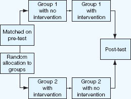
This is the Solomon design, intended to identify the interaction effect that may occur if the subject deduces the desired result from looking at the pre-test and the post-test. It is the same as the randomized controlled trial above, except that there are two control groups instead of one. In the standard randomized controlled trial any change in the experimental group can be due to the intervention or the pre-test, and any change in the control group can be due to the pre-test. In the Solomon variant the second control group receives the intervention but no pre-test. This can be modelled thus:
Experimental |
RO1 |
X |
O2 |
Control |
R03 |
|
O4 |
Control2 |
|
X |
O5 |
Thus any change in this second control group can only be due to the intervention. We refer readers to Bailey (1994: 231-4) for a full explication of this technique and its variants.
Here participants are randomly assigned to a control group and an experimental group, but there is no pretest. The experimental group receives the intervention and the two groups are given only a post-test. The design is:
Experimental |
R1 |
X |
O1 |
Control |
R2 |
|
O2 |
Here participants are randomly assigned to each of two experimental groups. Experimental group 1 receives intervention 1 and experimental group 2 receives intervention 2. Only post-tests are conducted on the two groups. The design is:
Experimental1 |
R1 |
X1 |
O1 |
Experimental2 |
R2 |
X2 |
O2 |
Here participants are randomly allocated to each of two experimental groups. Experimental group 1 receives intervention 1 and experimental group 2 receives intervention 2. Pre-tests and post-tests are conducted to measure changes in individuals in the two groups. The design is:
Experimental1 |
RO1 |
X1 |
O2 |
Experimental2 |
R02 |
X2 |
O4 |
The true experiment can also be conducted with one control group and two or more experimental groups. So, for example, the designs might be:
Experimental1 |
ROl |
X1 |
O2 |
Experimental2 |
R03 |
X2 |
O4 |
Control |
RO5 |
X |
O6 |
This can be extended to the post-test control and experimental group design and the post-test two experimental groups design, and the pre-test-post-test two treatment design.
As the name suggests, here participants are allocated to control and experimental groups randomly, but the basis of the allocation is that one member of the control group is matched to a member of the experimental group on the several independent variables considered important for the study (e.g. those independent variables that are considered to have an influence on the dependent variable, such as sex, age, ability). So, first, pairs of participants are selected who are matched in terms of the independent variable under consideration (e.g. whose scores on a particular measure are the same or similar), and then each of the pair is randomly assigned to the control or experimental group. Randomization takes place at the pair rather than the group level. Though, as its name suggests, this ensures effective matching of control and experimental groups, in practice it may not be easy to find sufficiently close matching, particularly in a field experiment, though finding such a close match in a field experiment may increase the control of the experiment considerably. Matched pairs designs are useful if the researcher cannot be certain that individual differences will not obscure treatment effects, as it enables these individual differences to be controlled.
Borg and Gall (1979: 547) set out a useful series of steps in the planning and conduct of an experiment:
Step 1: Carry out a measure of the dependent variable.
Step 2: Assign participants to matched pairs, based on the scores and measures established from Step 1.
Step 3: Randomly assign one person from each pair to the control group and the other to the experimental group.
Step 4: Administer the experimental treatment/intervention to the experimental group and, if appropriate, a placebo to the control group. Ensure that the control group is not subject to the intervention.
Step 5: Carry out a measure of the dependent variable with both groups and compare/measure them in order to determine the effect and its size on the dependent variable.
Borg and Gall (1979) indicate that difficulties arise in the close matching of the sample of the control and experimental groups. This involves careful identification of the variables on which the matching must take place. They suggest (p. 547) that matching on a number of variables that correlate with the dependent variable is more likely to reduce errors than matching on a single variable. The problem, of course, is that the greater the number of variables that have to be matched, the harder it is actually to find the sample of people who are matched. Hence the balance must be struck between having too few variables such that error can occur, and having so many variables that it is impossible to draw a sample. Instead of matched pairs, random allocation is possible, and this is discussed below.
Mitchell and Jolley (1988: 103) pose three important questions that researchers need to consider when comparing two groups:
Are the two groups equal at the commencement of the experiment?
Would the two groups have grown apart naturally, regardless of the intervention?
To what extent has initial measurement error of the two groups been a contributory factor in differences between scores?
Borg and Gall draw attention to the need to specify the degree of exactitude (or variance) of the match. For example, if the subjects were to be matched on, say, linguistic ability as measured in a standardized test, it is important to define the limits of variability that will be used to define the matching (e.g. ± 3 points). As before, the greater the degree of precision in the matching here, the closer will be the match, but the greater the degree of precision the harder it will be to find an exactly matched sample.
One way of addressing this issue is to place all the subjects in rank order on the basis of the scores or measures of the dependent variable. Then the first two subjects become one matched pair (which one is allocated to the control group and which to the experimental group is done randomly, e.g. by tossing a coin), subjects three and four become the next matched pair, subjects five and six become the next matched pair, and so on until the sample is drawn. Here the loss of precision is counterbalanced by the avoidance of the loss of subjects.
The alternative to matching that has been discussed earlier in the chapter is randomization. Smith (1991: 215) suggests that matching is most widely used in quasi-experimental and non-experimental research, and is a far inferior means of ruling out alternative causal explanations than randomization.
In an experiment there may be two or more independent variables acting on the dependent variable. For example, performance in an examination may be a consequence of availability of resources (independent variable one: limited availability, moderate availability, high availability) and motivation for the subject studied (independent variable two: little motivation, moderate motivation, high motivation). Each independent variable is studied at each of its levels (in the example here it is three levels for each independent variable). Participants are randomly assigned to groups that cover all the possible combinations of levels of each independent variable, for example:
Independent variable |
Level 1 |
Level 2 |
Level 3 |
Availability of resources |
limited availability (1) |
moderate availability (2) |
high availability (3) |
Motivation for the subject studied |
little motivation (4) |
moderate motivation (5) |
high motivation (6) |
Here the possible combinations are: 1+4, 1+5, 1+6, 2+4, 2 + 5, 2+6, 3+4, 3 + 5 and 3+6. This yields nine groups (3x3 combinations). Pre-tests and post-tests or post-tests only can be conducted. It might show, for example, that limited availability of resources and little motivation had a statistically significant influence on examination performance, whereas moderate and high availability of resources did not, or that high availability and high motivation had a statistically significant effect on performance, whereas high motivation and limited availability did not, and so on.
This example assumes that there are the same numbers of levels for each independent variable; this may not be the case. One variable may have, say, two levels, another three levels, and another four levels. Here the possible combinations are 2 x 3 x 4 = 24 levels and, therefore, 24 experimental groups. One can see that factorial designs quickly generate several groups of participants. A common example is a 2 x 2 design, in which two independent variables each have two values (i.e. four groups). Here experimental group 1 receives the intervention with independent variable 1 at level 1 and independent variable 2 at level 1; experimental group 2 receives the intervention with independent variable 1 at level 1 and independent variable 2 at level 2; experimental group 3 receives the intervention with independent variable 1 at level 2 and independent variable 2 at level 1; experimental group 4 receives the intervention with independent variable 1 at level 2 and independent variable 2 at level 2.
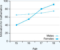
Factorial designs also have to take account of the interaction of the independent variables. For example one factor (independent variable) may be ‘sex’ and the other ‘age’ (Figure 16.3). The researcher may be investigating their effects on motivation for learning mathematics.
In Figure 16.3 one can see that the difference in motivation for mathematics is not constant between males and females, but that it varies according to the age of the participants. There is an interaction effect between age and sex, such that the effect of sex depends on age. A factorial design is useful for examining interaction effects.
At their simplest, factorial designs may have two levels of an independent variable, e.g. its presence or absence, but, as has been seen here, it can become more complex. That complexity is bought at the price of increasing exponentially the number of groups required.
Here participants are randomly assigned to groups whose parameters are fixed in terms of the levels of the independent variable that each receives. For example, let us imagine that an experiment is conducted to improve the reading abilities of poor, average, good and outstanding readers (four levels of the independent variable ‘reading ability’). Four experimental groups are set up to receive the intervention, thus: experimental group 1 (poor readers); experimental group 2 (average readers), experimental group 3 (good readers) and experimental group 4 (outstanding readers). The control group (group 5) would receive no intervention. The researcher could chart the differential effects of the intervention on the groups, and thus have a more sensitive indication of its effects than if there was only one experimental group containing a wide range of reading abilities; the researcher would know which group was most and least affected by the intervention. Parametric designs are useful if an independent variable is considered to have different levels or a range of values which may have a bearing on the outcome (confirmatory research) or if the researcher wishes to discover whether different levels of an independent variable have an effect on the outcome (exploratory research).
Here participants in the experimental groups are tested under two or more experimental conditions. So, for example, a member of the experimental group may receive more than one ‘intervention’, which may or may not include a control condition. This is a variant of the matched pairs design, and offers considerable control potential, as it is exactly the same person receiving different interventions. Order effects raise their heads here: the order in which the interventions are sequenced may have an effect on the outcome; the first intervention may have an influence – a carry-over effect – on the second, and the second intervention may have an influence on the third and so on. Further, early interventions may have a greater effect than later interventions. To overcome this it is possible to randomize the order of the interventions and assign participants randomly to different sequences, though this may not ensure a balanced sequence. Rather, a deliberate ordering may have to be planned, for example, in a three-intervention experiment:
Group 1 receives intervention 1 followed by intervention 2, followed by intervention 3;
Group 2 receives intervention 2 followed by intervention 3, followed by intervention 1;
Group 3 receives intervention 3 followed by intervention 1, followed by intervention 2;
Group 4 receives intervention 1 followed by intervention 3, followed by intervention 2;
Group 5 receives intervention 2 followed by intervention 1, followed by intervention 3;
Group 6 receives intervention 3 followed by intervention 2, followed by intervention 1.
Repeated measures designs are useful if it is considered that order effects are either unimportant or unlikely (see Figure 16.4), or if the researcher cannot be certain that individual differences will not obscure treatment effects, as it enables these individual differences to be controlled.
Often in educational research, it is simply not possible for investigators to undertake true experiments, e.g. in random assignation of participants to control or experimental groups. Quasi-experiments are the stuff of field experimentation, i.e. outside the laboratory. At best, they may be able to employ something approaching a true experimental design in which they have control over what Campbell and Stanley (1963) refer to as ‘the who and to whom of measurement’ but lack control over ‘the when and to whom of exposure’, or the randomization of exposures – essential if true experimentation is to take place. These situations are quasi-experimental and the methodologies employed by researchers are termed quasi-experimental designs. (Kerlinger (1970) refers to quasi-experimental situations as ‘compromise designs’, an apt description when applied to much educational research where the random selection or random assignment of schools and classrooms is quite impracticable.)
Quasi-experiments come in several forms, for example:
pre-experimental designs: the one group pre-test-post-test design; the one-group post-tests only design; the non-equivalent post-test only design;
pre-test-post-test non-equivalent group design;
one-group time series.
We consider these below.
Very often, reports about the value of a new teaching method or interest aroused by some curriculum innovation or other reveal that a researcher has measured a group on a dependent variable (01), for example, attitudes towards minority groups, and then introduced an experimental manipulation (X), perhaps a ten-week curriculum project designed to increase tolerance of ethnic minorities. Following the experimental treatment, the researcher has again measured group attitudes (02) and proceeded to account for differences between pre-test and post-test scores by reference to the effects of X.
The one group pre-test-post-test design can be represented as:
Experimental |
O1 |
X |
O2 |
Suppose that just such a project has been undertaken and that the researcher finds that 02 scores indicate greater tolerance of ethnic minorities than O1 scores. How justified is she in attributing the cause of 01-02 differences to the experimental treatment (X), that is, the term’s project work? At first glance the assumption of causality seems reasonable enough. The situation is not that simple, however. Compare for a moment the circumstances represented in our hypothetical educational example with those which typically obtain in experiments in the physical sciences. A physicist who applies heat to a metal bar can confidently attribute the observed expansion to the rise in temperature that she has introduced because within the confines of her laboratory she has excluded (i.e. controlled) all other extraneous sources of variation (Pilliner, 1973).
The same degree of control can never be attained in educational experimentation. At this point readers may care to reflect upon some possible influences other than the ten-week curriculum project that might account for the 01-02 differences in our hypothetical educational example.
They may conclude that factors to do with the pupils, the teacher, the school, the classroom organization, the curriculum materials and their presentation, the way that the subjects’ attitudes were measured, to say nothing of the thousand and one other events that occurred in and about the school during the course of the term’s work, might all have exerted some influence upon the observed differences in attitude. These kinds of extraneous variables which are outside the experimenters control in one-group pre-test-post-test designs threaten to invalidate their research efforts. We later identify a number of such threats to the validity of educational experimentation.
Here an experimental group receives the intervention and then takes the post-test. Though this has some features of an experiment (an intervention and a post-test), the lack of a pre-test, of a control group, of random allocation and of controls renders this a flawed methodology.
Again, though this appears to be akin to an experiment, the lack of a pre-test, of matched groups, of random allocation and of controls renders this a flawed methodology.
One of the most commonly used quasi-experimental designs in educational research can be represented as:
Experimental |
O1 |
X |
O2 |
Control |
O3 |
|
O4 |
The dashed line separating the parallel rows in the diagram of the non-equivalent control group indicates that the experimental and control groups have not been equated by randomization – hence the term ‘non-equivalent’. The addition of a control group makes the present design a decided improvement over the one group pre-test-post-test design, for to the degree that experimenters can make E and C groups as equivalent as possible, they can avoid the equivocality of interpretations that plague the pre-experimental design discussed earlier. The equivalence of groups can be strengthened by matching, followed by random assignment to E and C treatments.
Where matching is not possible, the researcher is advised to use samples from the same population or samples that are as alike as possible (Kerlinger, 1970). Where intact groups differ substantially, however, matching is unsatisfactory due to regression effects which lead to different group means on post-test measures.
Here the one group is the experimental group, and it is given more than one pre-test and more than one post-test. The time series uses repeated tests or observations both before and after the treatment, which, in effect, enables the participants to become their own controls, which reduces the effects of reactivity. Time series allow for trends to be observed, and avoid reliance on only one single pre-testing and post-testing data collection point. This enables trends to be observed such as: no effect at all (e.g. continuing an existing upward, downward or even trend), a clear effect (e.g. a sustained rise or drop in performance), delayed effects (e.g. some time after the intervention has occurred). Time series studies have the potential to increase reliability.
At the beginning of Chapter 14, we described case study researchers as typically engaged in observing the characteristics of an individual unit, be it a child, a classroom, a school or a whole community. We went on to contrast case study researchers with experimenters whom we described as typically concerned with the manipulation of variables in order to determine their causal significance. That distinction, as we shall see, is only partly true.
Increasingly, in recent years, single-case research as an experimental methodology has extended to such diverse fields as clinical psychology, medicine, education, social work, psychiatry and counselling. Most of the single-case studies carried out in these (and other) areas share the following characteristics:
they involve the continuous assessment of some aspect of human behaviour over a period of time, requiring on the part of the researcher the administration of measures on multiple occasions within separate phases of a study;
they involve ‘intervention effects’ which are replicated in the same subject(s) over time.
Continuous assessment measures are used as a basis for drawing inferences about the effectiveness of intervention procedures.
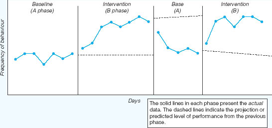
The characteristics of single-case research studies are discussed by Kazdin (1982) in terms of ABAB designs, the basic experimental format in most single-case researches. ABAB designs, Kazdin observes, consist of a family of procedures in which observations of performance are made over time for a given client or group of clients. Over the course of the investigation, changes are made in the experimental conditions to which the client is exposed. The basic rationale of the ABAB design is illustrated in Figure 16.5. What it does is this. It examines the effects of an intervention by alternating the baseline condition (the A phase), when no intervention is in effect, with the intervention condition (the B phase). The A and B phases are then repeated to complete the four phases. As Kazdin says, the effects of the intervention are clear if performance improves during the first intervention phase, reverts to or approaches original baseline levels of performance when the treatment is withdrawn, and improves again when treatment is recommenced in the second intervention phase.
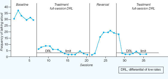
An example of the application of the ABAB design in an educational setting is provided by Dietz (1977) whose single-case study sought to measure the effect that a teacher could have upon the disruptive behaviour of an adolescent boy whose persistent talking disturbed his fellow classmates in a special education class.
In order to decrease the unwelcome behaviour, a reinforcement programme was devised in which the boy could earn extra time with the teacher by decreasing the number of times he called out. The boy was told that when he made three (or fewer) interruptions during any 55-minute class period the teacher would spend extra time working with him. In the technical language of behaviour modification theory, the pupil would receive reinforcing consequences when he was able to show a low rate of disruptive behaviour (in Figure 16.6 this is referred to as ‘differential reinforcement of low rates’ or DRL).
When the boy was able to desist from talking aloud on fewer than three occasions during any timetabled period, he was rewarded by the teacher spending 15 minutes with him helping him with his learning tasks. The pattern of results displayed in Figure 16.6 shows the considerable changes that occurred in the boy’s behaviour when the intervention procedures were carried out and the substantial increases in disruptions towards baseline levels when the teacher’s rewarding strategies were withdrawn. Finally, when the intervention was reinstated, the boy’s behaviour is seen to improve again.
The single-case research design is uniquely able to provide an experimental technique for evaluating interventions for the individual subject. Moreover, such interventions can be directed towards the particular subject or group and replicated over time or across behaviours, situations or persons. Single-case research offers an alternative strategy to the more usual methodologies based on between-group designs. There are, however, a number of problems that arise in connection with the use of single-case designs having to do with ambiguities introduced by trends and variations in baseline phase data and with the generality of results from single-case research. The interested reader is directed to Kazdin (1982), Borg (1981) and Vasta (1979).2
An experimental investigation must follow a set of logical procedures. Those that we now enumerate, however, should be treated with some circumspection. It is extraordinarily difficult (and foolhardy) to lay down clear-cut rules as guides to experimental research. At best, we can identify an ideal route to be followed, knowing full well that educational research rarely proceeds in such a systematic fashion.3
First, the researcher must identify and define the research problem as precisely as possible, always supposing that the problem is amenable to experimental methods.
Second, she must formulate hypotheses that she wishes to test. This involves making predictions about relationships between specific variables and at the same time making decisions about other variables that are to be excluded from the experiment by means of controls. Variables, remember, must have two properties. First, they must be measurable. Physical fitness, for example, is not directly measurable until it has been operationally defined. Making the variable ‘physical fitness’ operational means simply defining it by letting something else that is measurable stand for it – a gymnastics test, perhaps. Second, the proxy variable must be a valid indicator of the hypothetical variable in which one is interested. That is to say, a gymnastics test probably is a reasonable proxy for physical fitness; height on the other hand most certainly is not. Excluding variables from the experiment is inevitable, given constraints of time and money. It follows therefore that one must set up priorities among the variables in which one is interested so that the most important of them can be varied experimentally whilst others are held constant.
Third, the researcher must select appropriate levels at which to test the independent variables. By way of example, suppose an educational psychologist wishes to find out whether longer or shorter periods of reading make for reading attainment in school settings (see Simon, 1978). She will hardly select 5-hour and 5-minute periods as appropriate levels; rather, she is more likely to choose 30-minute and 60-minute levels, in order to compare with the usual timetabled periods of 45 minutes’ duration. In other words, the experimenter will vary the stimuli at such levels as are of practical interest in the real-life situation. Pursuing the example of reading attainment somewhat further, our hypothetical experimenter will be wise to vary the stimuli in large enough intervals so as to obtain measurable results. Comparing reading periods of 44 minutes, or 46 minutes, with timetabled reading lessons of 45 minutes is scarcely likely to result in observable differences in attainment.
Fourth, the researcher must decide which kind of experiment she will adopt, perhaps from the varieties set out in this chapter.
Fifth, in planning the design of the experiment, the researcher must take account of the population to which she wishes to generalize her results. This involves her in decisions over sample sizes and sampling methods. Sampling decisions are bound up with questions of funds, staffing and the amount of time available for experimentation. However, one general rule of thumb is to try to make the sample as large as possible so that even small effects can reveal themselves which might otherwise be lost with small samples, even though the trade-off here is that, with large samples, it is easier to achieve statistical significance (i.e. it is easier to find a statistically significant difference between the control group and the experimental group) than it is with a small sample (statistical significance being, in part, a function of sample size), though measures of effect size overcome this problem. Second, it is important, where possible, to use a random, probability sample, as this not only permits a greater range of statistics to be used (e.g. t-tests and analysis of variance, both of which are important in experiments, see Chapter 36), but it also enables the findings to have greater generalizability (external validity), i.e. to represent the wider population.
Sixth, with problems of validity in mind, the researcher must select instruments, choose tests and decide upon appropriate methods of analysis (typically t-tests and measures of effect size are used to determine whether there are any statistically significant or sizeable differences that are worthy of note, respectively, between the control and experimental groups).
Seventh, before embarking upon the actual experiment, the researcher must pilot test the experimental procedures to identify possible snags in connection with any aspect of the investigation. This is of crucial importance.
Eighth, during the experiment itself, the researcher must endeavour to follow tested and agreed-on procedures to the letter. The standardization of instructions, the exact timing of experimental sequences, the meticulous recording and checking of observations – these are the hallmark of the competent researcher.
With her data collected, the researcher faces the most important part of the whole enterprise. Processing data, analysing results and drafting reports are all extremely demanding activities, both in intellectual effort and time. Often this last part of the experimental research is given too little time in the overall planning of the investigation. Experienced researchers rarely make such a mistake; computer program faults and a dozen more unanticipated disasters teach the hard lesson of leaving ample time for the analysis and interpretation of experimental findings.
A ten-step model for the conduct of the experiment can be suggested:
Step 1: Identify the purpose of the experiment.
Step 2: Select the relevant variables.
Step 3: Specify the level(s) of the intervention (e.g. low, medium, high intervention).
Step 4: Control the experimental conditions and environment.
Step 5: Select the appropriate experimental design.
Step 6: Administer the pre-test.
Step 7: Assign the participants to the group(s).
Step 8: Conduct the intervention.
Step 9: Conduct the post-test.
Step 10: Analyse the results.
The sequence of steps 6 and 7 can be reversed; the intention in putting them in the present sequence is to ensure that the two groups are randomly allocated and matched. In experiments and fixed designs, data are aggregated rather than related to specific individuals, and data look for averages, the range of results, and their variation. In calculating differences or similarity between groups at the stages of the pre-test and the post-test, the t-test for independent samples is often used.
Chapter 10 indicted several threats to the internal and external validity of experiments, and we refer the reader to this chapter. In that chapter threats to internal validity (the validity of the research design, process, instrumentation and measurement) were seen to reside in:
history
maturation
statistical regression
testing
instrumentation
selection
experimental mortality
instrument reactivity
selection-maturation interaction
Type I and Type II errors.
To this, Hammersley (2008: 4) adds the point that not all the confounding variables may be properly controlled in the randomization process.
In Chapter 10, too, threats to external validity (wider generalizability) were seen to reside in:
failure to describe independent variables explicitly
lack of representativeness of available and target populations
Hawthorne effect
inadequate operationalizing of dependent variables
sensitization/reactivity to experimental/research conditions
interaction effects of extraneous factors and experimental/research treatments
invalidity or unreliability of instruments
ecological validity
multiple treatment validity.
To this, Hamnmersley (2008: 4) adds the point that, in principle, a laboratory trial, in which variables are controlled, misrepresents the ‘real’ world of the classroom in which the variables are far less controlled, i.e. the findings may not be transferable to wider conditions and situations.
One can add to these factors the matter that statistical significance can be found comparatively easily if sample sizes are large (Kline, 2004) (hence the need to consider placing greater reliance on effect size rather than statistical significance, discussed in Chapter 17). Further, Torgerson and Torgerson (2003a: 70-1) draw attention to the limits of small samples in experimental research, as small samples can fail to spot small effects, thereby risking a Type II error (failing to find an effect when, in fact, it exists). As they remark, in a time of evidence-based education and discussions of ‘what works’, small effects can be useful (p. 70), and they give the example where, if a small change in delivering the curriculum led to improved examination passes of only one child in each class in public examinations, then this could total up to between 20,000 and 30,000 students across the UK.
Torgerson and Torgerson (2003b) also identify several sources of bias in randomized controlled trials, for example:
a Having a very selective sample (they give the example of an exclusive girls-only boarding school) and then seeking to generalize the results to a much wider population, e.g. an inner-city mixed sex comprehensive (non-selective) school (p. 37).
b A selection bias, where the experimental group possesses a variable that is related to the outcome variable but which is not included in the intervention (pp.37-8).
c A dilution bias, where the control group, not being exposed to the intervention, deliberately seeks out a ‘compensating treatment’ (p. 38). For example, there may be an experiment to test the effects of increased attention to mathematics in the classroom on mathematics results in public examinations; the control group, not being exposed to what they see as a useful intervention (given that there has to be informed consent), may take private mathematics lessons in order to compensate, thereby disturbing or diluting the findings of the experiment.
d Chance effects: the authors give an example of a group of 40 children learning spellings, in which four of them were dyslexic, and in which the likelihood of them being randomly allocated to the control group and experimental group evenly (two in each group) was very small, indeed all four could be in one group (either the experimental group or the control group). The researchers argue that this can be addressed through ‘minimisation’ (p. 40), deliberately ensuring an even split of such students into both groups (e.g. matched pairs allocation).
e ‘Subversion bias’ (p. 40), where researchers deliberately breach the requirements of random allocation (hence the need for double-blind experiments or where the researcher is not involved in the randomized allocation).
f Attrition bias: Torgerson and Torgerson (2003a: 74-5) draw attention to the problem of attrition in experimental methods, where some students could drop out of the experimental group (they give the example of students who attend voluntary Saturday morning ‘booster classes’ and then who drop out of the class). Here, if the researchers only focused on the results of those students who remained in the Saturday morning classes, then they would obtain very different results from those which might have been found if the dropouts had not dropped out (e.g. in terms of measured motivation levels and, hence, achievement). There is a risk, the authors aver, of ‘attrition bias’ here (p. 75).
g Reporting or detection bias: where different researchers or reporters for the control and experimental groups report with differing degrees of detail or inclusion of relevant observations (Torgerson and Torgerson, 2003b: 42).
h Exclusion bias, where members of the experimental group for reasons other than attrition, do not actually take part in the experiment.
Experiments typically suffer from the problem of only having two time points for measurement: the pre-test and the post-test. It is essential that the researcher plans the timing of the pre-test and the post-test appropriately. Morrison (2009: 168) writes that ‘experimental procedures are prone to problems of timing – too soon and the effect may not be noticed; too late and the effect might have gone or been submerged by other matters’. The pretest should be conducted as close to the start of the intervention as possible, to avoid the influence of confounding effects between the pre-test and the start of the intervention; that is quite straightforward.
More difficult is the issue of the timing of the post-test. On the one hand the argument is strong that it should be as close as possible to the end of the intervention, as this will reduce the possibility of the influence of confounding effects. On the other hand, it may well be that the effects of a particular intervention may not reveal themselves immediately, but much later, for example a student may study Shakespeare at age 15 and, on an outcome measure, may use it to say that she strongly dislikes English literature, but, years later, she may point back to her study of Shakespeare as sowing the seed for her eventual love of Shakespeare that only developed after she had left school. Too soon the post-test and that effect is lost, it goes unmeasured (and this is a serious problem for the ‘what works’ movement that appears to concern itself with short-term payback).
On the other hand, too long a time lapse, and it becomes impossible to determine whether it was a particular independent variable that caused a particular effect, or whether other factors have intervened since the intervention to produce the effect.
Further still, it is possible that an immediate post-test could easily find an effect, but the effect is not sustained to any worthwhile degree over time. A standard example of this is where an end of course examination is administered at the last session of the course, or within a week of its completion, and, unsurprisingly perhaps, given the ‘recency effect’ (in which most recently studied items are more easily recalled than items studied a long time previously), many students score well. However, let us imagine that the post-test (the examination) had been conducted one month later, in which case the students might well have bleached the subject matter from their minds. Or, more problematic in this instance is the familiar case of students revising hard before the post-test (the examination) is administered, and they score well, but this time it is not a consequence of the intervention but a rehearsal, practice or revision effect.
One way in which the researcher can overcome the difficulty of the timing of the post-test is to have more than one post-test (e.g. an ‘equivalent form’ of the post-test: see Chapter 10), with the post-test administered soon after the intervention has ended, and its equivalent form administered after a longer period of time – to determine more long-lasting effects.
A pre-experimental design was used in a study involving the 1991-92 Postgraduate Diploma in Education group following a course of training to equip them to teach social studies in senior secondary schools in Botswana. The researcher wished to find out whether the programme of studies he had devised would effect changes in the students’ orientations towards social studies teaching. To that end, he employed a research instrument, the Barth/Shermis Studies Preference Scale (BSSPS) which has had wide use in differing cultures including America, Egypt and Nigeria, and whose construction meets commonly required criteria concerning validity and internal consistency reliability.
The BSSPS consists of 45 Likert-type items (Chapter 20), providing measures of what purport to be three social studies traditions or philosophical orientations, the oldest of which, Citizenship Transmission, involves indoctrination of the young in the basic values of a society. The second orientation, called the Social Science, is held to relate to the acquisition of knowledge-gathering skills based on the mastery of social science concepts and processes. The third tradition, Reflective Enquiry, is said to derive from John Dewey’s pragmatism with its emphasis on the process of enquiry. Forty-eight Postgraduate Diploma students were administered the BSSPS during the first session of their one-year course of study. At the end of the programme, the BSSPS was again completed in order to determine whether changes had occurred in students’ philosophical orientations. Briefly, the ‘preferred orientation’ in the pre-test and post-test was the criterion measure, the two orientations least preferred being ignored. Broadly speaking, students tended to move from a majority holding a Citizenship Transmission orientation at the beginning of the course to a greater affirmation of the Social Science and the Reflective Enquiry traditions. Using the symbols and conventions adopted earlier to represent research designs, we can illustrate the Botswana study as:
Experimental |
O1 |
X |
O2 |
The briefest consideration reveals inadequacies in the design. Indeed, Campbell and Stanley (1963) describe the one group pre-test-post-test design as ‘a “bad example” to illustrate several of the confounded extraneous variables that can jeopardize internal validity’. The investigator is rightly cautious in his conclusions: ‘it is possible to say that the social studies course might be responsible for this phenomenon, although other extraneous variables might be operating’ (Adeyemi, 1992, emphasis added). Somewhat ingenuously he puts his finger on one potential explanation, that the changes could have occurred among his intending teachers because the shift from ‘inculcation to rational decisionmaking was in line with the recommendation of the Nine Year Social Studies Syllabus issued by the Botswana Ministry of Education in 1989’ (Adeyemi, 1992).
Mason et al.’s (1992) longitudinal study took place between 1984 and 1992. Its principal aim was to test whether the explicit teaching of linguistic features of GCSE textbooks, coursework and examinations would produce an improvement in performance across the secondary curriculum. The title of their report, ‘Illuminating English: how explicit language teaching improved public examination results in a comprehensive school’, suggests that the authors were persuaded that they had achieved their objective. In light of the experimental design selected for the research, readers may ask themselves whether or not the results are as unequivocal as reported.
The design adopted in the Shevington study (Shevington is the location of the experiment in north-west England) may be represented as:
Experimental |
O1 |
X |
O2 |
Control |
O3 |
|
O4 |
This is, of course, the non-equivalent control group design outlined earlier in this chapter in which parallel rows separated by dashed lines represent groups that have not been equated by random assignment.
In brief, the researchers adopted a methodology akin to teaching English as a foreign language and applied this to Years 7-9 in Shevington Comprehensive School and two neighbouring schools, monitoring the pupils at every stage and comparing their performance with control groups drawn both from Shevington and the two other schools. Inevitably, because experimental and control groups were not randomly allocated, there were significant differences in the performance of some groups on pre-treatment measures such as the York Language Aptitude Test. Moreover, because no standardized reading tests of sufficient difficulty were available as post-treatment measures, tests had to be devised by the researchers, who provide no details as to their validity or reliability. These difficulties notwithstanding, pupils in the experimental groups taking public examinations in 1990 and 1991 showed substantial gains in respect of the percentage increases of those obtaining GCSE Grades A to C. The researchers note that during the three years 1989 to 1991, ‘no other significant change in the policy, teaching staff or organization of the school took place which could account for this dramatic improvement of 50 per cent’ (Mason et al., 1992).
Although the Shevington researchers attempted to exercise control over extraneous variables, readers may well ask whether threats to internal and external validity such as those alluded to earlier were sufficiently met as to allow such a categorical conclusion as, ‘the pupils ... achieved greater success in public examinations as a result of taking part in the project’ (Mason et al., 1992).
Another investigation (Bhadwal and Panda, 1991) concerned with effecting improvements in pupils’ performance as a consequence of changing teaching strategies used a more robust experimental design. In rural India, the researchers drew a sample of 78 pupils, matched by socio-economic backgrounds and non-verbal IQs, from three primary schools that were themselves matched by location, physical facilities, teachers’ qualifications and skills, school evaluation procedures and degree of parental involvement. Twenty-six pupils were randomly selected to comprise the experimental group, the remaining 52 being equally divided into two control groups. Before the introduction of the changed teaching strategies to the experimental group, all three groups completed questionnaires on their study habits and attitudes. These instruments were specifically designed for use with younger children and were subjected to the usual item analyses, test-retest and split-half reliability inspections. Bhadwal and Panda’s research design can be represented as:
Experimental |
ROl |
X |
R02 |
First control |
R03 |
|
R04 |
Second control |
RO5 |
|
R06 |
Recalling Kerlinger’s (1970) discussion of a ‘good’ experimental design, the version of the pre-test-post-test control design employed here (unlike the design used in Example 2 above) resorted to randomization which, in theory, controls all possible independent variables. Kerlinger adds, however, ‘in practice, it is only when enough subjects are included in the experiment that the principle of randomization has a chance to operate as a powerful control’. It is doubtful whether 26 pupils in each of the three groups in Bhadwal and Panda’s study constituted ‘enough subjects’.
In addition to the matching procedures in drawing up the sample, and the random allocation of pupils to experimental and control groups, the researchers also used analysis of covariance, as a further means of controlling for initial differences between E and C groups on their pre-test mean scores on the independent variables, study habits and attitudes.
The experimental programme involved improving teaching skills, classroom organization, teaching aids, pupil participation, remedial help, peer-tutoring and continuous evaluation. In addition, provision was also made in the experimental group for ensuring parental involvement and extra reading materials. It would be startling if such a package of teaching aids and curriculum strategies did not effect significant changes in their recipients and such was the case in the experimental results. The Experimental Group made highly significant gains in respect of its level of study habits as compared with Control Group 2 where students did not show a marked change. What did surprise the investigators, we suspect, was the significant increase in levels of study habits in Control Group 1. Maybe, they opined, this unexpected result occurred because Control Group 1 pupils were tested immediately prior to the beginning of their annual examinations. On the other hand, they conceded, some unaccountable variables might have been operating. There is, surely, a lesson here for all researchers! (For a set of examples of problematic experiments see the website material.)
The design experiment is perhaps more fittingly termed a ‘design study’, as it frequently does not conform to the requirements of an experiment (e.g. it does not have the hallmarks of a randomized controlled trial), as set out in the earlier part of this chapter. Design-based research is not the same as an experiment, though, in many circles, it has been termed (misleadingly) a design experiment. Hence it is included in this chapter because of its nomenclature rather than its affinity to experiments as described so far in this chapter, though, like an experiment, it involves a deliberate and planned intervention. It has appeared comparatively recently in education (e.g. Brown, 1992), and it was given the imprimatur of status in a special issue of Educational Researcher in 2003 (vol. 32 (1)).
It is more useful to focus on the word ‘design’ rather than ‘experiment’ here, as a design study owes some of its pedigree to engineering and science rather than to an experiment that has control and experimental groups. Brown (1992: 141) suggests that design studies attempt to ‘engineeer innovative educational environments and simultaneously conduct experimental studies of those innovations’. Take the example of engineering: here the designer develops a product and then tests it in real conditions (Gorard et al., 2004: 576), noting, during the testing (the experiment) what are the problems with the design, what needs to be improved, where there are faults and failures, and so on, gathering data from other participants and users. Then the engineer redesigns the product to address the faults found, refines the product and retests the improved product, noting faults, problems or failures; the engineer reworks the product to address these problems, and tests it out again, and so on. We can observe here:
1 The process is iterative; it has many cycles, trials, improvements and refinements over time.
2 It focuses on the processes involved in the workings of the product.
3 It communicates with different parties (theoreticians, designers, practitioners), about the design and development of the product (the designers, the engineers, the users), akin to a research-and-development model.
4 The product has to work in the ‘real world’ (an example of ‘what works’) and in non-laboratory conditions and contexts.
5 It is data-driven – the next cycle of refinement is based on data (e.g. observational data, measurement data, notes and records) derived from the previous round.
These points accord with key principles of design studies in education (Design-Based Research Collective, 2003: 5), for example in developing learning environments:
1 They intertwine theory, models and practice.
2 Research and development occur in cycles of refinement, testing and feedback (‘design, enactment and analysis’ (Design-Based Research Collective, 2003: 6)).
3 The findings must be communicated and shared with all parties, including the users.
4 The research and the outcomes must be tested and used in authentic, real-world settings respectively.
5 Reporting and development go together in developing a useable outcome.
Shavelson et al. (2003: 26) suggest that key principles of design studies are that they are: (a) ‘iterative’; (b) ‘process focused’; (c) ‘interventionist’; (d) ‘collaborative’; (e) ‘multileveled’; (f) ‘utility oriented’; and (g) ‘theory driven’. Cobb et al. (2003: 9) suggest that theory generation is a key feature of design experiments; they are ‘crucibles for the generation and testing of theory’ (p. 9), their purpose is to generate theories of teaching and learning (p. 10), and this involves development, intervention and reflection. In having ‘pragmatic roots’ (p. 10), Cobb et al. point us to suggesting the affinity between design experiments and mixed methods research (see Chapter 1), and, indeed, this is echoed by Gorard et al. (2004: 579, 593).
The inception of design studies is often attributed to Brown (1992), whose autobiographical account of her years of research charts a movement away from the laboratory and into the classroom, in order to catch the authenticity of the real world in research and development. She recognizes that this is bought at the price of tidiness, and she justifies this in terms of the real world being ‘rarely isolatable’ in terms of its components, and in which ‘the whole really is more than the sum of its parts’ (p. 166). For her and her successors, interventions are based on theoretical claims (e.g. about teaching and learning) (for example Design-Based Research Collective, 2003: 5) and are inextricably linked to practices that improve the situation (e.g. of teaching and learning); they respond to ‘emergent features’ of the situation in which they are operating (Design-Based Research Collective, 2003: 6). Practitioners, researchers and developers work together to produce a useful intervention and innovation.
A design-base study is a study that focuses on changing practice, instead of the static, ‘frozen’ (Design-Based Research Collective, 2003: 7) input-output model of an intervention that one sees in much experimental and educational research, in a design study the ‘product’ changes over time, as refinements are made in response to feedback from all parties.
However, unlike an engineering product, a design-base study does not end with the perfecting of a particular product. Rather, as Brown (1992) indicated, it affects theory, e.g. of learning, of teaching. The design-based study can address and generate many kinds of knowledge (Design-Based Research Collective, 2003: 8):
investigating possibilities for new and innovative teaching environments;
developing theories of teaching and learning that are rooted in real-world contexts;
developing cumulative knowledge of design;
increasing capacity in humans for innovation.
To this Shavelson et al. (2003: 28) suggest that design studies can address research that asks ‘what is happening?’, ‘is there a systematic effect?’ and ‘why or how is it happening?’.
The attraction of the approach is that it takes account of the complex, real, multivariate world of learning, teaching and education; as such they are ‘messier’ than conventional experiments, as they take account of many variables and contexts, the intervention develops and changes over time and involves several parties and strives to ensure that what works at the design stage really works in practice (Gorard et al., 2004: 578, 582). The design study develops a profile of multiple variables rather than testing a sole hypothesis (Lobato, 2003: 19).
On the other hand Shavelson et al. (2003) argue that design studies are not exempted the usual warrants of research, for example, they ask ‘what is the basis of knowing in design studies’ (p. 25), ‘with so many confounding variables in a design study, can the knowledge claims be warranted’ (p. 27), how generalizable the results can be, as they are so rooted in specific contexts (p. 27), and how have alternative explanations of the outcomes been considered (p. 27). To answer these questions, McCandliss et al. (2003: 15) also add that video recording can provide useful data over time, and Shavelson et al. (2003) suggest that longitudinal narrative data are particularly useful as they can track developments and causal developments over time in a way that catches the complexity and contextualization of the intervention which inheres in its very principles. However, narrative accounts risk circularity, and there need to be external checks and balances, controls and warrants, in validating the knowledge claims (p. 27).
Further, Sloane and Gorard (2003) indicate some difficulties that design studies have to address, including measurement problems, external validity, the lack of controls and control groups, the lack of failure criteria (and they argue that engineers include failure criteria as essential features of their research and development), and the need for appropriate modelling of causality at both the alpha stages (the designers) and the beta stages (the users). Hence researchers using a design study have to be clear on its purposes, intended contribution to theory generation, participants and communication processes between them, processes of intervention and debriefing/feedback, clear understanding of the local context of the intervention (Cobb et al., 2003: 12), and ‘testable conjectures’ that can be revised iteratively (Cobb et al., 2003: 11).
A growing field in psychological research is the use of the internet for experiments (e.g. www.psych.unizh.ch/genpsy/Ulf/Lab/webExpPsyLab.html). Hewson et al. (2003: 48) classify these into four principal types: ‘those that present static printed materials (for example, printed text or graphics); second are those that make use of non-printed materials (for example, video or sound); third are reaction-time experiments; and fourth are experiments that involve some form of interpersonal interaction’.
The first kind of experiment is akin to a survey in that it sends formulated material to respondents (e.g. graphically presented material) by email or by web page, and the intervention will be to send different groups different materials. Here all the cautions and comments that were made about internet-based surveys apply, particularly those problems of download times, different browsers and platforms. However, the matter of download time applies more strongly to the second type of internet-based experiments that use video clips or sound, and some software packages will reproduce higher quality than others, even though the original that is transmitted is the same for everyone. This can be addressed by ensuring that the material runs at its optimum even on the slowest computer (Hewson et al., 2003: 49) or by stating the minimum hardware required for the experiment to be run successfully.
Reaction-time experiments, those that require very precise timing (e.g. to milliseconds) are difficult in remote situations, as different platforms and internet connection speeds and congestion on the internet through having multiple users at busy times can render standardization virtually impossible. One solution to this is to have the experiment downloaded and then run offline before loading it back onto the computer and sending it.
The fourth type involves interaction, and is akin to internet interviewing (discussed below), facilitated by chat rooms. However, this is solely a written medium and so intonation, inflection, hesitancies, non-verbal cues, extra-linguistic and paralinguistic factors are ruled out of this medium. It is, in a sense, incomplete, though the increasing availability and use of simple screen-top video cameras is mitigating this. Indeed this latter development renders observational studies an increasing possibility in the internet age.
Reips (2002a) reports that in comparison to laboratory experiments, internet-based experiments experienced greater problems of dropout, that the dropout rate in an internet experiment was very varied (from 1 per cent to 87 per cent), and that dropout could be reduced by offering incentives, e.g. payments or lottery tickets, bringing a difference of as much as 31 per cent to dropout rates. Dropout on internet-based research was due to a range of factors, for example motivation, how interesting the experiment was, not least of which was the non-compulsory nature of the experiment (in contrast, for example, to the compulsory nature of experiments undertaken by university student participants as part of their degree studies). The discussion of the ‘high hurdle technique’ earlier is applicable to experiments here. Reips (2002b: 245-6) also reports that greater variance in results is likely in an internet-based experiment than in a conventional experiment due to technical matters (e.g. network connection speed, computer speed, multiple software running in parallel). He also reports (Reips, 2009: 381) that internet experiments suffer from reducing the controls that the experimenter can place on the participant, and the problems of a biased, volunteer-only sample (p. 382) or recruitment biases.
On the other hand Reips (2002b: 247) also reports that internet-based experiments have an attraction over laboratory and conventional experiments in that they:
have greater generalizability because of their wider sampling;
demonstrate greater ecological validity as typically they are conducted in settings that are familiar to the participants and at times suitable to the participant (‘the experiment comes to the participant, not vice versa’), though, of course, the obverse of this is that the researcher has no control over the experimental setting (p. 250);
they have a high degree of voluntariness, such that more authentic behaviours can be observed.
How correct these claims are is an empirical matter. For example, the use of sophisticated software packages (e.g. Java) can reduce experimenter control as these packages may interact with other programming languages. Indeed Schwarz and Reips (2001) report that the use of Javascript led to a 13 per cent higher dropout rate in an experiment compared to an identical experiment that did not use Javascript. Further, multiple returns by a single participant could confound reliability (discussed above in connection with survey methods).
Reips (2002a, 2002b) provides a series of ‘dos’ and ‘don’ts’ in internet experimenting. In terms of ‘dos’ he gives five main points:
1 use dropout as a dependent variable;
2 use dropout to detect motivational confounding (i.e. to identify boredom and motivation levels in experiments);
3 place questions for personal information at the beginning of the internet study. Reips (2002b) suggests that asking for personal information may assist in keeping participants in an experiment, and that this is part of the ‘high hurdle’ technique, where dropouts self-select out of the study, rather than dropping out during the study;
4 use techniques that help ensure quality in data collection over the internet (e.g. the ‘high hurdle’ and ‘warm-up’ techniques discussed earlier, subsampling to detect and ensure consistency of results, using single passwords to ensure data integrity, providing contact information, reducing dropout);
5 use internet-based tools and services to develop and announce your study (using commercially produced software to ensure that technical and presentational problems are overcome). There are also websites (e.g. the American Psychological Society) that announce experiments.
In terms of ‘don’ts’ he gives five main points:
1 Do not allow external access to unprotected directories. This can violate ethical and legal requirements, as it provides access to confidential data. It also might allow the participants to have access to the structure of the experiment, thereby contaminating the experiment.
2 Do not allow public display of confidential participant data through URLs (a problem if respondents use the GET protocol), as this, again, violates ethical codes.
3 Do not accidentally reveal the experiment’s structure (as this could affect participant behaviour). This might be done through including the experiment’s details on a related file or a file in the same directory.
4 Do not ignore the technical variance inherent in the internet (configuration details, browsers, platforms, bandwidth and software might all distort the experiment, as discussed above).
5 Do not bias results through improper use of form elements (i.e. measurement errors, where, by omitting particular categories (e.g. ‘neutral’, ‘do not want to respond’, ‘neither agree nor disagree’) could distort the results).
Indeed, the points made in connection with internet surveys and questionnaires apply equally to internet experiments, and readers are advised to review these.
Reips (2002b) points out that it is a misconception to regard an internet-based experiment as the same as a laboratory experiment, as: (a) internet participants could choose to leave the experiment at any time; (b) they can conduct the experiment at any time and in their own settings; (c) they are often conducted with larger samples than conventional experiments; (d) they rely on technical matters, network connections and the computer competence of the participants; and (e) they are more public than most conventional experiments. On the other hand he also cautions against regarding the internet-based experiment as completely different from the laboratory experiment, as: (a) many laboratory experiments also rely on computers; (b) fundamental ideas are the same for laboratory and internet-based surveys; (c) similar results have been produced by both means. He suggests several issues in conducting internet-based experiments:
1 Consider a web-based software tool to develop the experimental materials.
2 Pilot the experiment on different platforms for clarity of instructions and availability on different platforms.
3 Decide the level of sophistication of HTML scripting and whether to use HTML or non-HTML.
4 Check the experiments for configuration errors and variance on different computers.
5 Place the experiment on several websites and services.
6 Run the experiment online and offline to make comparisons.
7 Use the ‘warm-up’ and ‘high hurdle’ techniques, asking filter questions (e.g. about the seriousness of the participant, their background and expertise, language skills).
8 Use dropout to ascertain whether there is motivational confounding.
9 Check for obvious naming of files and conditions (to reduce the possibility of unwanted access to files).
10 Consider using passwords and procedures (e.g. consistency checks) to reduce the possibility of multiple submissions.
11 Keep an experimental log of data for any subsequent analysis and verification of results.
12 Analyse and report dropout.
13 Keep the experimental details on the internet, to give a positive impression of the experiment.
Reips (2009: 375) also writes that the success of internet-based experimentation depends in part on the ‘cues transmitted’, the ‘bandwidth’, ‘cost constraints’, ‘level and type of anonymity’ and ‘synchronicity and exclusivity’ (see also Birnbaum, 2009).
At the time of writing, the internet-based experiment is currently more a child of psychology than of education. However, given the rise of evidence-based practice in education, and the advocacy of randomized controlled trials in education, this form of experimentation is set to become more widely used in education.
Details of the development of internet-based experimental software can be found at:
www.genpsylab.unizch/wextor/index.html
http://psych.hanover.edu.APS/exponnet.html
www.genpsy.unizch/Ulf.Lab/webexplist.html.
We also refer readers to Joinson et al. (2009), Part Five.
This chapter has introduced a range of different types of experiment. Starting with the ‘true’ experiment, it held this up as the clearest example of a full experiment, as it abides by all the features of an experiment, in particular it adheres to the tenets of a randomized controlled trial, which is intended to yield evidence of ‘what works’. The strengths and limitations of the true experiment and the randomized controlled trial were set out. Further variants of a true experiment were set out. Moving further out of the laboratory and into the ‘real world’, the chapter then presented a discussion of different types of quasi-experiment, i.e. those kinds of experiment in which not all the requirements of a true experiment were met or, in the case of ex post facto experiments or those which could not be justified on ethical or practical grounds, where the requirements of a true experiment were impossible to meet. Rendering an experiment a quasi-experiment rather than a true experiment was seen to lie not only in design matters, but in issues of sampling and controls. Moving yet further into the ‘real world’ the chapter ended by introducing design experiments, or, as was argued to be more fittingly described, a design study.
 Companion Website
The companion website to the book includes PowerPoint slides for this chapter, which list the structure of the chapter and then provide a summary of the key points in each of its sections. In addition there is further information in the form of examples of experiments. These resources can be found online at www.routledge.com/textbooks/cohen7e.