Modeling Biogeochemical Cycles
4.1 Introductory Remarks
To formulate a model is to put together pieces of knowledge about a particular system into a consistent pattern that can form the basis for (1) interpretation of the past history of the system and (2) prediction of the future of the system. To be credible and useful, any model of a physical, chemical or biological system must rely on both scientific fundamentals and observations of the world around us. High-quality observational data are the basis upon which our understanding of the environment rests. However, observations themselves are not very useful unless the results can be interpreted in some kind of model. Thus observations and modeling go hand in hand.
This chapter focuses on types of models used to describe the functioning of biogeochemical cycles, i.e., reservoir or box models. Certain fundamental concepts are introduced and some examples are given of applications to biogeochemical cycles. Further examples can be found in the chapters devoted to the various cycles. The chapter also contains a brief discussion of the nature and mathematical description of exchange and transport processes that occur in the oceans and in the atmosphere. This chapter assumes familiarity with the definitions and basic concepts listed in Section 1.5 of the introduction such as reservoir, flux, cycle, etc.
Modeling biogeochemical cycles normally involves estimating the spatial and temporal averages for concentrations and fluxes in and out of reservoirs (i.e., reservoir modeling). The spatial average (i.e., the physical size of the reservoir itself) often has a horizontal size approaching that of a continent, or larger, i.e., > 1000 km. The time scales corresponding to this spatial average are months, or longer. This means that day-to-day variations in weather and ocean currents are not generally considered explicitly when modeling biogeochemical cycles.
The advent of fast computers and the availability of detailed data on the occurrence of certain chemical species have made it possible to construct meaningful cycle models with a much smaller and faster spatial and temporal resolution. These spatial and time scales correspond to those in weather forecast models, i.e. down to 100 km and 1 h. Transport processes (e.g., for CO2 and sulfur compounds) in the oceans and atmosphere can be explicitly described in such models. These are often referred to as “tracer transport models.” This type of model will also be discussed briefly in this chapter.
4.2 Time Scales and Single Reservoir Systems
4.2.1 Turnover Time
Consider the reservoir shown in Fig. 4-1. The turnover time is the ratio between the content (M) of a substance (tracer) in the reservoir and the total flux out of it (S):

Fig. 4-1 Schematic illustration of a single reservoir with source flux Q, sink flux S, and content M.
The turnover time may be thought of as the time it would take to empty the reservoir if the sink (S) remained constant while the sources were zero (τ0S=M). This time scale is also sometimes referred to as “renewal time” or “flushing time.” In the common case when the sink is proportional to the reservoir content (S=kM), the turnover time is the inverse of the proportionality constant (k−1), which is analogous to first-order chemical kinetics.
In fluid reservoirs like the atmosphere or the ocean, the turnover time of a tracer is also related to the spatial and temporal variability of its concentration within the reservoir; a long turnover time corresponds to a small variability and vice versa (Junge, 1974; Hamrud, 1983). Figure 4-2 shows a plot of measured trace gas variability in the atmosphere versus turnover time estimated by applying budget considerations as indicated by Equation (1). An inverse relation is obvious, but the scatter in the data implies some departure from this simple relation.
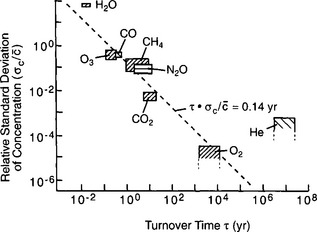
Fig. 4-2 Inverse relationship between relative standard deviation of atmospheric concentration and turnover time for important trace chemicals in the troposphere. (Modified from Junge (1974) with permission from the Swedish Geophysical Society.)
If material is removed from the reservoir by two or more separate processes, each with a flux Si, then turnover times with respect to each process can be defined as:
Since Σ Si=S, these time scales are related to the turnover time of the reservoir, τ0, by
As an application of the turnover time concept, let us consider the model of the carbon cycle shown in Fig. 4-3. This diagram is different from the one used in the chapter on the carbon cycle ( Chapter 11), because it serves our purposes better for this chapter. The values given for the various fluxes and burdens are very similar to the corresponding figure in Chapter 11 ( Fig. 11-1).
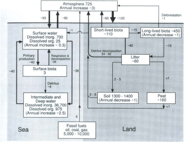
Fig. 4-3 Principal reservoirs and fluxes in the carbon cycle. Units are 1015 g (Pg) C (burdens) and Pg C/yr (fluxes). (From Bolin (1986) with permission from John Wiley and Sons.)
The turnover time of carbon in biota in the ocean surface water is 3 × 10¹⁵/(4 + 36) × 1015 yr ≈ 1 month. The turnover time with respect to settling of detritus to deeper layers is considerably longer: 9 months. Faster removal processes in this case must determine the turnover time: respiration and decomposition.
The equation describing the rate of change of the content of a reservoir can be written as
If the reservoir is in a steady state (dM/dt = 0) then the sources (Q) and sinks (S) must balance. In this case Q can replace S in Equation (1).
4.2.2 Residence Time (Transit Time)
The residence time is the time spent in a reservoir by an individual atom or molecule. It is also the age of a molecule when it leaves the reservoir. If the pathway of a tracer from the source to the sink is characterized by a physical transport, the word transit time can also be used. Even for a single chemical substance, different atoms and molecules will have different residence times in a given reservoir. Let the probability density function of residence times be denoted by ϕ(τ), where ϕ(τ)dτ. describes the fraction of the tracer having a residence time in the interval to τ to τ + dτ. The average residence time (average transit time) τr is defined by:
In many cases the word “average” is left out and this quantity is simply referred to as “residence time.”
The shape of the probability density function, ϕ(τ), depends on the system. Some examples are shown in Fig. 4-4. This figure also contains probability density of age (see Section 4.2.3). Figure 4-4a might correspond to a lake with inlet and outlet on opposite sides of the lake. Most water molecules will then have a residence time in the lake roughly equal to the time it takes for the mean current to carry the water from the inlet to the outlet, i.e., τr. Very few molecules will have a residence time much greater than or much less than τr, as illustrated in the ϕ curve. Another example is a human population where most people live to attain mature age. The ϕ curve in this case can be interpreted as the frequency function for the age at which people die; few die very young and few survive the average age of death by more than 50%.
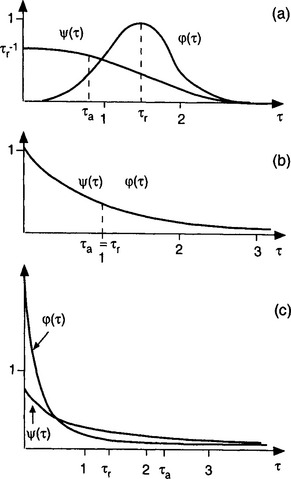
Fig. 4-4 The age frequency function ψ(τ) and the residence time frequency function ϕ(τ) and the corresponding average values τa and τr for the three cases described in the text: (a) τa > τr; (b) τa = τr; (c) τa > τr. (Adapted from Bolin and Rodhe (1973) with permission from the Swedish Geophysical Society.)
Figure 4-4b illustrates exponential decay. A simple example could be the reservoir of all 238U on Earth. The half-life of this radionuclide is 4.5 × 10⁹ years. Since the Earth is approximately 4.5 × 10⁹ years old, this implies that the content of the 238U reservoir today is about half of what it was when the Earth was formed. The probability density function of residence time of the uranium atoms originally present is an exponential decay function. The average residence time is 6.5 × 10⁹ years. (The average value of time for an exponential decay function is the half-life divided by ln 2.) In a well-mixed reservoir all particles always have the same probability of being removed. In such situations the frequency function for the residence time is also exponential.
In the reservoir corresponding to Fig. 4-4c the removal is biased towards “young” particles. This might occur when the sink is located close to the source (the “short circuit” case).
4.2.3 Age
The age of an atom or molecule in a reservoir is the time since it entered the reservoir. As with residence times, the probability density function of ages, ψ(τ), has a shape that depends on the situation. In a steady-state reservoir, however, ψ(τ) is always a nonincreasing function. The shapes of ψ(τ) corresponding to the three residence time distributions discussed above are included in Fig. 4-4.
4.2.4 Relations Between τ0,τr and τa
It can be shown that for a reservoir in steady state, τ0 is equal to τr, i.e. the turnover time is equal to the average residence time spent in the reservoir by individual particles (Eriksson, 1971; Bolin and Rodhe, 1973). This may seem to be a trivial result but it is actually of great significance. For example, if τ0 can be estimated from budget considerations by comparing fluxes and burdens in Equation (1) and if the average transport velocity (V) within the reservoir is known, the average distance (L=Vτr) over which the transport takes place in the reservoir can be estimated.
The relation between τ0 and τa is not as simple. τa may be larger or less than τ0 depending on the shape of the age probability density function (as shown in Fig. 4-4). For a well-mixed reservoir, or one with a first-order removal process, τa = τ0 (Fig. 4-4b).
In the case of a human population corresponding to Fig. 4-4a, τa is only about half of τ0 This example applies to the average age of all Swedes, which is around 40 years, whereas the average residence time, i.e., the average length of life (average age at death) is almost 80 years.
In the situation where most atoms leave the reservoir soon and few of them remain very long (Fig. 4-4c), τa is larger than τ0 (the “short circuit” case). Some further examples of age distributions and relations between τa and τ0 are given in Lerman (1979).
When equating τ0 and τr it must be made clear that the flux, S, which defines τ0 (see Equation (1)) is the gross flux and not a net flux. For example, removal of water from the atmosphere occurs both by precipitation and dry deposition (direct uptake by diffusion to the surface). Dry deposition is not normally explicitly evaluated but subtracted from the gross evaporation flux to yield the net evaporation from the surface. The turnover time of water in the atmosphere calculated as the ratio between the atmospheric content and the precipitation rate (about 10 days) is thus not equal to the average residence time of water molecules in the atmosphere. The actual value of the average residence time of individual water molecules is substantially shorter.
4.2.5 Response Time
The response time (relaxation time, adjustment time) of a reservoir is a time scale that characterizes the adjustment to equilibrium after a sudden change in the system. A precise definition is not easy to give except in special circumstances like in the following example.
Consider a single reservoir, like the one shown in Fig. 4-1, for which the sink is proportional to the content (S=kM) and which is initially in a steady state with fluxes Q0 = S0 and content M0. The turnover time of this reservoir is
Suppose now that the source strength is suddenly changed to a new value Q1. How long would it take for the reservoir to reach a new steady state? The adjustment process is described by the differential equation
with the initial condition M(t = 0) = M0.
approaches the new steady-state value (M1 = Q1/k) with a response time equal to k−1 or τ0. The change of the reservoir mass from the initial value M0 to the final value M1 is illustrated in Fig. 4-5. In this case, with an exponential adjustment, the response time is defined as the time it takes to reduce the imbalance to e−1 = 37% of the initial imbalance. This time scale is sometimes referred to as “e-folding time.” Thus, for a single reservoir with a sink proportional to its content, the response time equals the turnover time.
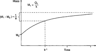
Fig. 4-5 Illustration of an exponential adjustment process. In this case, the response time is equal to k−1.
As a specific example, consider oceanic sulfate as the reservoir. Its main source is river runoff (pre-industrial value: 100 Tg S/yr) and the sink is probably incorporation into the lithosphere by hydrogeothermal circulation in mid-ocean ridges (100 Tg S/yr, McDuff and Morel, 1980). This is discussed more fully in Chapter 13. The content of sulfate in the oceans is about 1.3 × 10⁹ Tg S. If we make the (unrealistic) assumption that the present runoff, which due to man-made activities has increased to 200 Tg S/yr, would continue indefinitely, how fast would the sulfate concentration in the ocean adjust to a new equilibrium value? The time scale characterizing the adjustment would be τ0 ≈ 1.3 × 10⁹ Tg/(102 Tg/yr) ≈ 107 years and the new equilibrium concentration eventually approached would be twice the original value. A more detailed treatment of a similar problem can be found in Southam and Hay (1976).
4.2.6 Reservoirs in Non-steady State
Let us analyze the situation when one observes a change in reservoir content and wants to draw conclusions regarding the sources and sinks. We rewrite Equation (8) as
where τ0= 1/k is the turnover time in the steady state situation. Let us denote the left side of the equation (the observed rate of change of the reservoir content) as τ−1obs. If the mass were observed to increase by, say, 1% per year, τobs would be 100 years. Two limiting cases can be singled out:
1. τobs  τ0. In this case there has to be an approximate balance between the two terms on the right-hand side of the equation.
This means that the observed change in M mainly reflects a change in the source flux Q or the sink function. As an example we may take the methane concentration in the atmosphere, which in recent years has been increasing by about 0.5% per year. The turnover time is estimated to be about 10 years, i.e., much less than τobs (200 years). Consequently, the observed rate of increase in atmospheric methane is a direct consequence of a similar rate of increase of emissions into the atmosphere. (In fact, this is not quite true. A fraction of the observed increase is probably due to a decrease in sink strength caused by a decrease in the concentration of hydroxyl radicals responsible for the decomposition of methane in the atmosphere.)
2. τobs  τ0. In this case dM/dt ≈ Q which means that there is an increase in reservoir content about equal to the source flux with little influence on the part of the sink. The reservoir is then in an accumulative stage and its mass is increasing with time largely as a function of Q, irrespective of whether Q itself is increasing, decreasing or constant. A good example of this situation is sulfur hexafluoride (SF6) whose concentration in the atmosphere is currently increasing by about 0.5% per year (τobs = 200 years) as a result of various industrial emissions (IPCC, 1996). Because of inefficient removal processes (SF6is a very stable molecule) the turnover time of SF6 is as large as 3000 years. The rate of increase is thus a reflection of an imbalance between sources and sinks rather than an increase in the source flux Q.
In situations where τobs is comparable in magnitude to τ0, a more complex relation prevails between Q, S, and M. Atmospheric CO2 falls in this last category although its turnover time (3–4 years, cf. Fig. 4-3) is much shorter than τobs (about 300 years). This is because the atmospheric CO2 reservoir is closely coupled to the carbon reservoir in the biota and in the surface layer of the oceans (Section 4.3). The effective turnover time of the combined system is actually several hundred years (Rodhe and Björkström, 1979).
4.3 Coupled Reservoirs
The treatment of time scales and dynamic behavior of single reservoirs given in the previous section can easily be generalized to systems of two or more reservoirs. While the simple system analyzed in the previous section illustrates many important characteristics of cycles, most natural cycles are more complex. The matrix method described in Section 4.3.1 provides an approach to systems with very large numbers of reservoirs that is at least simple in notation. The treatments in the preceding section and in Section 4.3.1 are still limited to linear systems. In many cases we assume linearity because our knowledge is not adequate to assume any other dependence and because the solution of linear systems is straightforward. There are, however, some important cases where non-linearities are reasonably well understood. In such cases analytical mathematical solutions, corresponding to those given in Section 4.3.1, normally do not exist and the mathematical expressions describing the dynamics of the cycle have to be replaced by finite difference expressions that may be solved by computer. A few of these cases are described in Section 4.3.2.
As important as coupled reservoirs and nonlinear systems are, the less mathematically inclined may want to read this section only for its qualitative material. The treatment described here is not essential for understanding the material later in the book. However, an excellent overview of solving differential equations by the eigenvalue–eigenvector method used in the next section appears in Section 3.6 of Braun (1983).
4.3.1 Linear Systems
A linear system of reservoirs is one where the fluxes between the reservoirs are linearly related to the reservoir contents. A special case, that is commonly assumed to apply, is one where the fluxes between reservoirs are proportional to the content of the reservoirs where they originate. Under this proportionality assumption the flux Fij from reservoir i to reservoir j is given by
The rate of change of the amount Mi in reservoir i is thus
where n is the total number of reservoirs in the system.
This system of differential equations can be written in matrix form as
where the vector M is equal to (M1, M2,…, Mn) and the elements of matrix k are linear combinations of the coefficients kij. The solution to Equation (12) describes the adjustment of all reservoirs to a steady state by a finite sum of exponential decay functions (Lasaga, 1980; Chameides and Perdue, 1997). The time scales of the exponential decay factors correspond to the nonzero eigenvalues of the matrix k. The response time of the system, τcycle, may be defined by
where E1 is the nonzero eigenvalue with smallest absolute value (Lasaga, 1980). The treatment can be generalized by adding an external forcing function on the right-hand side of Equations (11) and (12).
As an illustration of the concept introduced above, let us consider a coupled two-reservoir system with no external forcing (Fig. 4-6). The dynamic behavior of this system is governed by the two differential equations
the expression of conservation of mass
and the initial condition
Equations (14) can be written in matrix form as
where M is the vector (M1, M2) describing the contents of the two reservoirs and k the matrix:
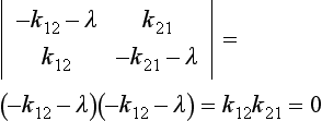
The eigenvalues of k are the solutions to the equation
λ1 = 0 and λ2 = –(k12 + k21). The general solution to Equation (17) can be written as
where ψ1 and ψ2 are the eigenvectors of the matrix k. In our case, we have
or, in component form and in terms of the initial conditions:
It is seen that in the steady state the total mass is distributed between the two reservoirs in proportion to the sink coefficients (in reverse proportion to the turnover times), independent of the initial distribution.

Fig. 4-6 A coupled two-reservoir system with fluxes proportional to the content of the emitting reservoirs.
In this simple case there is only one time scale characterizing the adjustment process, that is (k12 + k21)−1. This is also the response time, τcycle, as defined by Equation (13).
or, if expressed in terms of the turnover times of the two reservoirs:
The response time in this simple model will depend on the turnover times of both reservoirs and will always be shorter than the shortest of the two turnover times. If τ01 is equal to τ02, then τcycle will be equal to half of this value.
An investigation of the dynamic behavior of a coupled three-reservoir system using the techniques described above is included in the problems listed at the end of the chapter.
It should be noted that the steady-state solution of Equation (12) is not necessarily unique. This can easily be seen in the case of the four-reservoir system shown in Fig. 4-7. In the steady state all material will end up in the two accumulating reservoirs at the bottom. However, the distribution between these two reservoirs will depend on the amount initially located in the two upper reservoirs.
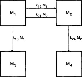
Fig. 4-7 Example of a coupled reservoir system where the steady-state distribution of mass is not uniquely determined by the parameters describing the fluxes within the system but also by the initial conditions (see text).
Before turning to nonlinear situations, let us consider two specific examples of coupled linear systems. The first describes the dynamic behavior of a multireservoir system; the second represents a steady-state situation of an open two-reservoir system.
Example 1. As a specific example of a time-dependent linear system we may take the model of the phosphorus cycle shown in Fig. 4-8. This is a duplicate of the figure shown in the chapter on the phosphorous cycle (Fig. 14-7). The authors used a computer to solve the system of equations in Equation (11) with a time-dependent source term added to represent the transient situation with an exponentially increasing industrial mining input (7% increase per year). Lasaga (1980) studied the same situation in a more elegant way using matrix algebra. The evolution of the phosphorus content of the various reservoirs (except in sediments) during the first 70 years is shown in Table 4-1. Within this time frame, the only noticeable change is seen to occur in the land reservoir. Lasaga showed that the adjustment time scale of the system, τcycle, is 53 000 years. This is much shorter than the turnover time of the sediment reservoir (2 × 10⁸ years) but much longer than the turnover times of all other reservoirs. This cycle is described in greater detail in Chapter 14.
Table 4-1
Response of phosphorus cycle to mining output. Phosphorus amounts are given in Tg P (1 Tg = 1012 g). Initial contents and fluxes as in Fig. 4-7 (system at steady state). In addition, a perturbation is introduced by the flux from reservoir 7 (mineable phosphorus) to reservoir 2 (land phosphorus), which is given by 12 exp(0.07t) in units of Tg P/yr

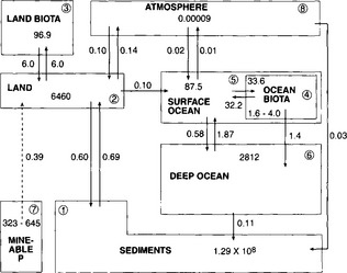
Fig. 4-8 The global phosphorus cycle. Values shown are in Tmol and Tmol/yr. (Adapted from Lerman et al. (1975) and modified to include atmospheric transfers. The mass of P in each reservoir and rates of exchange are taken from Jahnke (1992), MacKenzie et al. (1993) and Follmi (1996).)
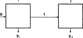
Example 2. As a much simpler example let us consider a system consisting of two connected reservoirs as depicted in Fig. 4-9. Steady state is assumed to prevail. Material is introduced at a constant rate Q into reservoir 1. Some of this material is removed (S1) and the rest (T) is transferred to reservoir 2, from which it is removed at a rate S2. The turnover times (average residence times) of the two reservoirs and of the combined reservoir (defined as the sum of the two reservoirs) are easily calculated to be
where α = T/Q is the fraction of the material passing through reservoir 1 that is transferred to reservoir 2. An example application of this two-reservoir model is that it has been used to study the oxidation of sulfur in the atmosphere where SO2–sulfur was treated as one reservoir and sulfate–sulfur as the other (Rodhe, 1978). In the special case where S1 = 0, T=Q and α = 1 (all material introduced in reservoir 1 is transferred to reservoir 2) the turnover time of the combined reservoir equals the sum of the turnover times of the individual reservoirs.
4.3.2 Non-linear Systems
In many situations the assumption about linear relations between removal rates and reservoir contents is invalid and more complex relations must be assumed. No simple theory exists for treating the various non-linear situations that are possible. The following discussion will be limited to a few examples of non-linear reservoir/flux relations and cycles. For a more comprehensive discussion, see the review by Lasaga (1980).
Consider a single reservoir with a constant rate of supply and a removal rate proportional to the square of the reservoir content. The equation governing the rate of change of the reservoir content is
If M(0) = 0, the solution to this equation is
This is graphically illustrated in Fig. 4-10. Initially, the mass increases almost linearly with time. After the time the removal term becomes effective and the mass begins to level off. M eventually reaches a steady state equal to
 but the response time scale is not as easily defined as in the linear case. Relative to a simple exponential relaxation process the adjustment given by Equation (28) is more rapid initially, and slower as time progresses.
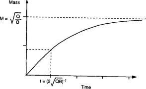
Fig. 4-10 The shape of the function given in Equation (28).
In general, if the removal flux is dependent upon the reservoir content raised to the power α (α ≠ 1), i.e., S=BMα, the adjustment process will be faster or slower than the steady-state turnover time depending on whether α is larger or smaller than unity (Rodhe and Björkström, 1979).
A similar simple non-linear adjustment process is described by the equation
which is a common model for the growth of biological systems (it is called logistical growth). The term AM represents exponential growth (unlimited supply of space and nutrients) and the term BM2 is a removal term, a negative feedback effect of “crowdedness.” Initially (where AM0 
 ), the growth will be close to exponential and will then gradually level off to the equilibrium value A/B (Fig. 4-11).
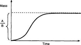
Fig. 4-11 Shape of “logistical growth.” The rate of change increases slowly initially. The rate of growth reaches a maximum and eventually drops to zero as the mass levels off, approaching the value A/B.
A sink flux that has a weaker than proportional dependence on the content M of the emitting reservoir is often described by the Michaelis–Menten equation:
where C is a rate coefficient and D a term (Michaelis constant) which determines the deviation from proportionality; a small D (compared to M) corresponds to a weak dependence of S on M and a large D corresponds to a near proportional dependence.
An important example of non-linearity in a biogeochemical cycle is the exchange of carbon dioxide between the ocean surface water and the atmosphere and between the atmosphere and the terrestrial system. To illustrate some effects of these non-linearities, let us consider the simplified model of the carbon cycle shown in Fig. 4-12. MS represents the sum of all forms of dissolved carbon (CO2, H2CO3, and
and ). The ocean to atmosphere flux, which is dependent on the concentration of the dissolved species CO2(aq), is related to the total carbon content in the surface layer (MS) by
where the exponent αSA (the buffer, or Revelle factor) is about 9. The buffer factor results from the equilibrium between CO2(g) and the more prevalent forms of dissolved carbon. This effect is discussed further in Chapter 11. As a consequence of this strong dependence of FSA on MS, a substantial increase in CO2 in the atmosphere is balanced by a small increase of MS.
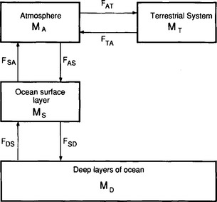
Fig. 4-12 Simplified model of the biogeochemical carbon cycle. (Adapted from Rodhe and Björkström (1979) with the permission of the Swedish Geophysical Society.)
Similarly, the flux from the atmosphere to the terrestrial system may be represented by the expression
The exponent αAT is considerably less than unity owing to the fact that CO2 generally is not the limiting factor for vegetation growth. This means that even a substantial increase in MA does not produce a corresponding increase in FAT.
Assuming that the carbon cycle of Fig. 4-12 will remain a closed system over several thousands of years, we can ask how the equilibrium distribution within the system would change after the introduction of a certain amount of fossil carbon. Table 4-2 contains the answer for two different assumptions about the total input. The first 1000 Pg corresponds to the total input from fossil fuel up to about the year 2000; the second (6000 Pg) is roughly equal to the now known accessible reserves of fossil carbon (Keeling and Bacastow, 1977).
Table 4-2
Steady-state carbon contents (unit: Pg = 1015 g) for the four-reservoir model of Fig. 4-11: (a) during the unperturbed (pre-industrial) situation; (b) after the introduction of 1000 Pg carbon; and (c) after the introduction of 6000 Pg carbon

If all fluxes are proportional to the reservoir contents, the percentage change in reservoir content will be equal for all the reservoirs. The non-linear relations discussed above give rise to substantial variations between the reservoirs. Note that the atmospheric reservoir is much more significantly perturbed than any of the other three reservoirs. Even in the case with a 6000 Pg input, the carbon content of the oceans does not increase by more than 12% at steady state.
However, with “only” 1000 Pg emitted into the system, i.e. less than 3% of the total amount of carbon in the four reservoirs, the atmospheric reservoir would still remain significantly affected (20%) at steady state. In this case the change in oceanic carbon would be only 2% and hardly noticeable. The steady-state distributions are independent of where the addition occurs. If the CO2 from fossil fuel combustion were collected and dumped into the ocean, the final distribution would still be the same.
If all fluxes were proportional to the reservoir content, i.e., if αSA and αAT were unity, all reservoirs would be equally affected; 15% in the 6000 Pg case and 2.5% in the 1000 Pg case.
4.4 Fluxes Influenced by the Receiving Reservoir
There are some important situations in which a flux between two reservoirs is determined not only by the mass of the emitting reservoir but also by the mass of the receptor. Uptake of CO2, or indeed any other nutrient by a plant community depends also on the magnitude of its biomass because that determines the size of the surfaces where photosynthesis take place. Consider, for example, the uptake of atmospheric CO2 by terrestrial biota. A reasonable parameterization of this flux would be
where the notations follow those in Fig. 4-12 with MTB being the content of carbon in terrestrial biota and D, a Michaelis constant. One problem with an expression like this is that mathematically speaking, the flux FAT and the mass MTB may grow without bounds; the larger MTB, the larger the flux to it, i.e., exponential growth. To avoid such a mathematical explosion, Williams (1987) suggested that the factor MTB in Equation (33) be replaced by
where MTBmax is an upper limit to the size of MTB. Once MTB approaches the value MTBmax′ the flux diminishes to zero and MTB is kept limited.
4.5 Coupled Cycles
An important class of cycles with non-linear behavior is represented by situations when coupling occurs between cycles of different elements. The behavior of coupled systems of this type has been studied in detail by Prigogine (1967) and others. In these systems, multiple equilibria are sometimes possible and oscillatory behavior can occur. There have been suggestions that atmospheric systems of chemical species, coupled by chemical reactions, could exhibit multiple equilibria under realistic ranges of concentration (Fox et al., 1982; White, 1984). However, no such situations have been confirmed by measurements.
The cycles of carbon and the other main plant nutrients are coupled in a fundamental way by the involvement of these elements in photosynthetic assimilation and plant growth. Redfield (1934) and several others have shown that there are approximately constant proportions of C, N, S, and P in marine plankton and land plants (“Redfield ratios”); see Chapter 10. This implies that the exchange flux of one of these elements between the biota reservoir and the atmosphere – or ocean – must be strongly influenced by the flux of the others.
Williams (1987) has pointed out that there are two main approaches to the treatment of such couplings. The first is to apply flux expressions like the one described for CO2 in Section 4.4, in Equation (33), and let both the rate coefficient (k) and the upper limit of the biota reservoir size (MTBmax) be explicit functions of the available concentrations of the other nutrients. This approach allows for a pronounced interdependence between the fluxes of the different nutrients but it does not ensure that the Redfield ratios are maintained. In the second approach the contents of the nutrients in the biota reservoir are forced to remain close to the Redfield ratios. This method was used by Mackenzie et al. (1993) in their study of the global cycles of C, N, P, and S and their interactions. They were able to demonstrate how a human perturbation in one of these element cycles could influence the cycles of the other elements.
4.6 Forward and Inverse Modeling
In most cases models describing biogeochemical cycles are used to estimate the concentration (or total mass) in the various reservoirs based on information about source and sink processes, as in the examples given in Section 4.4. This is often called forward modeling. If direct measurements of the concentration are available, they can be compared to the model estimates. This process is referred to as model testing. If there are significant differences between observations and model simulations, improvements in the model are necessary. A natural step is then to reconsider the specification of the sources and/or the sinks and perform additional simulations.
Inverse modeling represents a situation when a model is used, in a systematic fashion, to estimate the magnitude of sources or sinks from observed concentrations (mass). In the simplest case with a single reservoir (Fig. 4-1) in steady state, the formal solution of the inverse problem follows directly from the relations Q=kM or k=Q/M, depending on whether Q or k is the quantity being sought. In a situation when concentrations vary in space and time and the model consists of several reservoirs the inverse modeling becomes more complex and statistical methods, such as minimizing the squares of deviations between observations and simulations, have to be employed. For example, Prinn et al. (1992) used an eight-box model of the atmosphere (four latitude bands and two height layers) together with observations of methyl chloroform (CH3CCl3) from a global network and information about its emission rate to estimate the removal rate of this gas in the atmosphere. Since the only removal process for methyl chloroform is the reaction with hydroxyl radical and the rate of this chemical reaction is well established, their result also provided an estimate of the concentration of hydroxyl radical in the atmosphere. This estimate of the atmospheric concentration of hydroxyl radical has been very useful in connection with later (forward) modeling of many other chemical compounds that are also removed by reaction with the hydroxyl radical, e.g., CO, CH4, SO2, etc.
4.7 High-Resolution Models
So far the focus of this chapter has been on relatively simple box models with each box representing a reservoir with well-defined boundaries in terms of its physical, chemical or biological characteristics, e.g., the ocean surface layer, the atmosphere, the terrestrial biota, etc. In many situations it is also important to model the distribution of a species within such a reservoir, especially the fluid reservoirs (atmosphere and water bodies) where transport processes are rapid. A common tool for modeling such processes is a gridpoint model in which the fluid space is divided into smaller boxes, each one of them represented mathematically in the model by a single gridpoint. The physical transport of the species in question, by mean motions as well as by turbulence, can then be described according to Equations (40) and (41) in Section 4.8.1 if the spatial derivatives are approximated by finite differences between adjacent gridpoints.
The simplest kind of gridpoint model is one where only one spatial dimension is considered, most often the vertical. Such one-dimensional models are particularly useful when the conditions are horizontally homogeneous and the main transport occurs in the vertical direction. Examples of such situations are the vertical distribution of CO2 within the ocean (except for the downwelling regions in high latitudes, Siegenthaler, 1983) and the vertical distribution of ozone and other trace gases in the stratosphere (Ko et al., 1989).
Two-dimensional gridpoint models enable more realistic descriptions of transport processes in that circulation cells like the Hadley cell in the tropical and subtropical troposphere (cf. Section 10.5.2) can be explicitly modeled. Models of this kind, with height vs. latitude dimensions, have been very useful for improving our understanding of the global-scale distributions of long-lived gaseous components in the atmosphere. For species with an atmospheric lifetime that is short compared to the characteristic time for mixing longitudinally around the globe, i.e., several weeks, two-dimensional (height/latitude) models are less useful. This is the case for reactive gases like SO2 and NOx as well as for species carried by aerosol particles, which have average atmospheric lifetimes of only a few days. For such species the concentration also exhibits large variations in the longitudinal direction, so three-dimensional models (height/latitude/longitude) are required.
In three-dimensional models many more oceanic and atmospheric motion systems can be explicitly described, including ocean currents and monsoon circulations and extratropical cyclones in the atmosphere. The drawback is that these models quickly become very complex and require large computer facilities. This limitation has recently become less of a problem because of the rapid development of computers and the increasing number of high-quality observations for model testing. Indeed, regional and global scale three-dimensional models have become a standard tool for studies of biogeochemical cycles, especially their atmospheric component.
Although many important features of oceanic and atmospheric circulation can be explicitly resolved in three-dimensional gridpoint models, there will always be many processes that occur on the sub-gridscale level that cannot. The effects of these sub-gridscale processes must be parameterized, i.e., summarized in a statistical fashion in a way related to the large-scale flow. The purpose of parameterization is to describe the combined effect of sub-gridscale processes on the larger-scale variables. For example, convective motion systems in the oceans and in the atmosphere occur on spatial scales of a few km or less and therefore cannot be resolved explicitly in large-scale models with a grid size of 100 km or more. However, the combined effect of such motions is of fundamental importance for vertical energy transport. Parameterization schemes therefore have to be used to describe how convection develops under certain conditions and how they influence the large-scale flow in the ocean and in the atmosphere.
Figure 4-13 shows an example from a three-dimensional model simulation of the global atmospheric sulfur balance (Feichter et al., 1996). The model had a grid resolution of about 500 km in the horizontal and on average 1 km in the vertical. The chemical scheme of the model included emissions of dimethyl sulfide (DMS) from the oceans and SO2 from industrial processes and volcanoes. Atmospheric DMS is oxidized by the hydroxyl radical to form SO2, which, in turn, is further oxidized to sulfuric acid and sulfates by reaction with either hydroxyl radical in the gas phase or with hydrogen peroxide or ozone in cloud droplets. Both SO2 and aerosol sulfate are removed from the atmosphere by dry and wet deposition processes. The reasonable agreement between the simulated and observed wet deposition of sulfate indicates that the most important processes affecting the atmospheric sulfur balance have been adequately treated in the model.
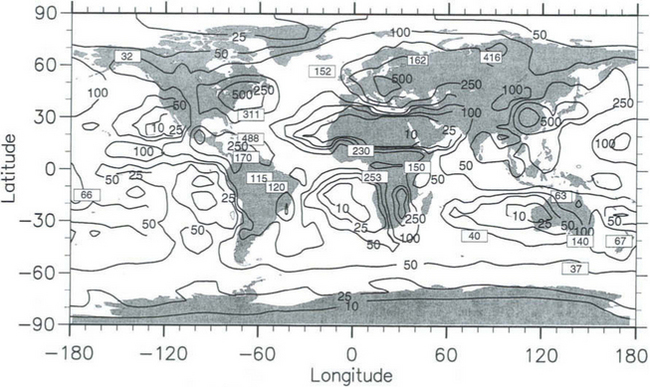
Fig. 4-13 Calculated and observed annual wet deposition of sulfur in mg S/m2 per year. (Reprinted from “Atmospheric Environment,” Volume 30, Feichter, J., Kjellström, E., Rodhe, H., Dentener, F., Lelieveld, J., and Roelofs, G.-J., Simulation of the tropospheric sulfur cycle in a global climate model, pp. 1693–1707, Copyright © 1996, with permission from Elsevier Science.)
In gridpoint models, transport processes such as speed and direction of wind and ocean currents, and turbulent diffusivities (see Section 4.8.1) normally have to be prescribed. Information on these physical quantities may come from observations or from other (dynamic) models, which calculate the flow patterns from basic hydrodynamic equations. Tracer transport models, in which the transport processes are prescribed in this way, are often referred to as off-line models. An on-line model, on the other hand, is one where the tracers have been incorporated directly into a dynamic model such that the tracer concentrations and the motions are calculated simultaneously. A major advantage of an on-line model is that feedbacks of the tracer on the energy balance can be described realistically. Examples of such dynamically interactive tracers that are important for the climate system are CO2 and the other greenhouse gases, as well as aerosols. Due to the great complexity of global models that combine in an interactive fashion tracer transport and explicit hydrodynamics, few such simulations have yet been carried out.
Dynamic models based on gridpoint or spectral discretization have been used by meteorologists to forecast weather for several decades. Today, the climate issue has stimulated rapid development of models designed for simulations of climate and its variations on time scales of decades and centuries. Unlike weather forecast models, global-scale climate models – general circulation models (GCMs) – must include descriptions of ocean circulation, the distribution of ice, snow and vegetation, and especially the exchange of heat, water and momentum (friction) between the atmosphere and the underlying surface. Figure 4-14 is a schematic of the components considered in a GCM.
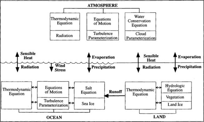
Fig. 4-14 Schematic diagram showing the components of a global climate model (GCM). (Reprinted from Hartmann (1994), with permission from Academic Press.)
4.8 Transport Processes
So far we have not gone in-depth into the nature of the transport processes responsible for fluxes of material between and within reservoirs. This section includes a very brief discussion of some of the processes that are important in the context of global biogeochemical cycles. More comprehensive treatments can be found in textbooks on geology, oceanography and meteorology and in reviews such as Lerman (1979) and Liss and Slinn (1983).
4.8.1 Advection, Turbulent Flux and Molecular Diffusion
Let us consider a fluid in which a tracer i ismixed. A flux of the tracer within the fluid can be brought about either by organized fluid motion or by molecular diffusion. These two flux processes can be written as
and
where Fi1 and Fi2 denote the flux vectors of the tracer (dimension: M/(L2T)), V the fluid velocity vector (L/T), ρ the density of the fluid (M/L3), qi the tracer mixing ratio (M/M), ci the mass concentration of the tracer (M/L3), D the molecular diffusivity (L2/T) and ∇ the gradient operator (L−1). The expression ∇qi: denotes the vector (∂qi/∂x, ∂qi/∂y, ∂qi/∂z).
The continuity of tracer mass is expressed by the equation
where Q and S represent production and removal of the tracer (M/(L3T)). Here ∇ · Fi denotes the scalar quantity
If variations in fluid density and diffusivity can be neglected we have
In most situations a fluid would be turbulent implying that the velocity vector, as well as the concentration ci, exhibits considerable variability on time scales smaller than those of prime interest. This situation can be described by writing these quantities as the sum of an average quantity (normally a time average) and a perturbation
From Equation (34), the transport flux Fi1, then becomes
and its average value
Note that the averages of V′ and c′ are equal to zero. The continuity equation can now be written as
The first two terms on the right side of Equation (40) describe the contributions from transport by advection and by turbulent flux, respectively. The separation of the motion flux into advection and turbulent flux is somewhat arbitrary; depending upon the circumstances the averaging time can be anything from a few minutes to a year or even more.
Since in most situations the perturbation quantities (V′ and c′i) are not explicitly resolved, it is not possible to evaluate the turbulent flux term directly. Instead, it must be related to the distribution of averaged quantities – a process referred to as parameterization. A common assumption is to relate the turbulent flux vector to the gradient of the averaged tracer distribution, which is analogous with the molecular diffusion expression, Equation (35).
The coefficient kturb introduced in Equation (41) (dimension: L2/T) is called the turbulent, or eddy diffusivity. In the general case the eddy diffusivity is given separate values for the three spatial dimensions. It must be remembered that the eddy diffusivities are not constants in any real sense (like the molecular diffusivities) and that their numerical values are very uncertain. The assumption underlying Equation (41) is therefore open to question.
In most cases, the term expressing the divergence of the molecular flux in Equation (40) can be neglected compared to the other two transport terms. Important exceptions occur, e.g. in a thin layer of the atmosphere close to the surface and in similar layers of the oceans close to the ocean floor and to the surface (viscous sublayers). Molecular diffusion is also an important transport process in the upper atmosphere, at heights above 100 km.
Order-of-magnitude values for the vertical eddy diffusivity in the atmosphere and the ocean are shown in Fig. 4-15. The values for the viscous layers represent molecular diffusivities of a typical air molecule like N2.
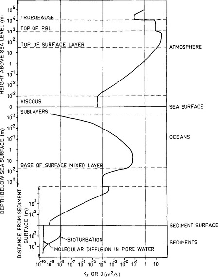
Fig. 4-15 Orders of magnitude of the average vertical molecular or turbulent diffusivity (whichever is largest) through the atmosphere, oceans, and uppermost layer of ocean sediments.
Development in recent years of fast-response instruments able to measure rapid fluctuations of the wind velocity (V’) and of the tracer concentration (c′), has made it possible to calculate the turbulent flux directly from the correlation expression in Equation (41), without having to resort to uncertain assumptions about eddy diffusivities. For example, Grelle and Lindroth (1996) used this eddy-correlation technique to calculate the vertical flux of CO2 above a forest canopy in Sweden. Since the mean vertical velocity has to vanish above such a flat surface, the only contribution to the vertical flux of CO2 comes from the eddy-correlation term
 In order to capture the contributions from all important eddies, both the anemometer and the CO2 instrument must be able to resolve fluctuations on time scales down to about 0.1 s.
A type of motion that is often very important in both the oceans and the atmosphere is convection. This is a vertical mixing process where parcels of water (or air) are rapidly transported in the vertical direction due to their buoyancy. In the oceans, this occurs when the surface water becomes denser than the underlying water – by cooling and/or increased salinity due to evaporation – and parcels of water sink down within days to depths of up to several km. In the atmosphere, convective motions occur when surface air is heated by conduction from the underlying surface. Air parcels having a horizontal dimension on the order of 1 km then rise and sometimes reach a height as high as 10–15 km within less than an hour, especially in tropical areas. Cumulus and cumulonimbus clouds are visible manifestations of convection in the atmosphere. In some circumstances, convection may contribute to a very rapid vertical mixing.
4.8.2 Other Transport Processes
Under some circumstances transport processes other than fluid motion and molecular diffusion are important. One important example is sedimentation due to gravity acting on particulate matter submerged in a fluid, e.g., removal of dissolved sulfur from the atmosphere by precipitation scavenging, or transport of organic carbon from the surface waters to the deep layers and to the sediment by settling detritus. The rate of transport by sedimentation is determined essentially by the size and density of the particles and by the counteracting drag exerted by the fluid.
Geochemically significant mixing and transport can sometimes be accomplished by biological processes. An interesting example is redistribution of sediment material caused by the movements of worms and other organisms (bioturbation).
Exchange processes between the atmosphere and oceans and between the oceans and the sediments are treated below in separate sections.
4.8.3 Air-Sea Exchange
4.8.3.1 Gas transfer
The magnitude and direction of the net flux density, F, of any gaseous species across an air-water interface is positive if the flux is directed from the atmosphere to the ocean. F is related to the difference in concentration (Δc), in the two phases by the relation
Here Δc = ca – KHcw with ca and cw representing the concentrations in the air and water respectively and KH the Henry’s law constant. The parameter K, linking the flux and the concentration difference, has the dimension of a velocity. It is often referred to as the transfer (or piston) velocity. The reciprocal of the transfer velocity corresponds to a resistance to transfer across the surface. The total resistance (R=K−1) can be viewed as the sum of an air resistance (Ra) and a water resistance (Rw):
The parameters ka and k1 are the transfer velocities for chemically unreactive gases through the viscous sublayers in the air and water, respectively. They relate the flux density F to the concentration gradients across the viscous sublayers through expressions similar to Equation (42):
Here ca,i and cw,i are the concentrations right at the interface (cf. Fig. 4-16). They are related by ca,i = KHcw,i.
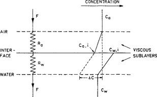
Fig. 4-16 A simplified model of flux resistances and concentration gradients in the viscous sublayers at the air-sea interface.
The parameter α in Equation (43) quantifies any enhancement in the value of k1 due to chemical reactivity of the gas in the water. Its value is unity for an unreactive gas; for gases with rapid aqueous phase reactions (e.g., SO2) much higher values can occur.
A comparison of the resistance in air and water for different gases shows that the resistance in the water dominates for gases with low solubility that are unreactive in the aqueous phase (e.g., O2, N2, CO2, CH4). For gases of high solubility or rapid aqueous chemistry (e.g., H2O, SO2, NH3) processes in the air control the interfacial transfer.
The numerical values of the transfer velocity K for the different gases are not well established. Its magnitude depends on such factors as wind speed, surface waves, bubbles and heat transfer. A globally averaged value of K often used for CO2 is about 10 cm/h. Transport at the sea-air interface is also discussed in Chapter 10; for a review see Liss (1983).
4.8.3.2 Transfer of particles
Liquid water, including its soluble and insoluble constituents, is transferred from the oceans to the atmosphere when air bubbles in the water rise to the surface. These bubbles form from air trapped by breaking waves, “whitecaps.” As the bubbles burst at the surface, water droplets are injected into the atmosphere. These water droplets are small enough to remain airborne for several hours. Whitecaps begin to form in winds common over the oceans, and a significant amount of seasalt made airborne in this way is transported to the continents and deposited in coastal areas.
The flux of particles in the other direction, deposition on the ocean surface, occurs intermittently in precipitation (wet deposition) and more continuously as a direct uptake by the surface (dry deposition). These flux densities may be represented by a product of the concentration of particulate matter in air close to the surface and parameters often referred to as deposition velocities:
The deposition velocities depend on the size distribution of the particulate matter, on the frequency of occurrence and intensity of precipitation, the chemical composition of the particles, the wind speed, nature of the surface, etc. Typical values of vw and vd for particles below about 1 µm in diameter are in the range 0.1 to 1 cm/s (Slinn, 1983). The average residence time in the atmosphere for such particles is a few days.
4.8.4 Sediment–Water Exchange
The sediment surface separates a mixture of solid sediment and interstitial water from the overlying water. Growth of the sediment results from accumulation of solid particles and inclusion of water in the pore space between the particles. The rates of sediment deposition vary from a few millimeters per 1000 years in the pelagic ocean up to centimeters per year in lakes and coastal areas. The resulting flux density of solid particles to the sediment surface is normally in the range 0.006 to 6 kg/m2 per year (Lerman, 1979). The corresponding flux density of materials dissolved in the trapped water is 10−6 to 10−3 kg/m2 per year. Chemical species may also be transported across the sediment surface by other transport processes. The main processes are (Lerman, 1979):
1. Sedimentation of solids (mineral, skeletal and organic materials).
2. Flux of dissolved material and water into sediment, contributing to the growth of the sediment column.
3. Upward flow of pore water and dissolved material caused by pressure gradients.
4. Molecular diffusional fluxes in pore water.
5. Mixing of sediment and water at the interface (bioturbation and water turbulence).
An estimate of the advective fluxes (processes 1, 2, and 3) requires knowledge of the concentration of the species in solutions and in the solid particles as well as of the rates of sedimentation and pore water flow. The diffusive type processes, 4 and 5, depend on vertical gradients of the concentrations of the species as well as on the diffusivities. In regions where bioturbation occurs, the effective diffusivity in the uppermost centimeters of the sediments can be more than that due to molecular diffusion in the pore water alone (cf. Fig. 4-15).
4.9 Time Scales of Mixing in the Atmosphere and Oceans
It is often important to know how long an element spends in one environment before it is transported somewhere else in the Earth system. For example, if a time scale characterizing a chemical or physical transformation process in a region has been estimated, a comparison with the time scale characterizing the transport away from the region will tell which process is likely to dominate.
The question of residence time and its definition in a steady-state reservoir was discussed earlier in this chapter. The average residence time in the reservoir was shown to be equal to the turnover time τ0 = M/S where M is the mass of the reservoir and S the total flux out of it. It is important to note that if one considers the exchange between two reservoirs of different mass, the time scale of exchange will be different depending upon whether the perspective is from the small or the big reservoir. An interesting example is that of mixing between the troposphere and stratosphere in the atmosphere. Studies of radioactive nuclides injected into the lower stratosphere by bomb testing have shown that the time scale characterizing the exchange between the lower stratosphere and troposphere is one to a few years. This means that a “particle” injected in the lower stratosphere will stay for this time, on average, before entering the troposphere. On the other hand, a gas molecule like N2O, which is chemically stable in the troposphere, will spend several decades in the troposphere before it is mixed up into the lower stratosphere, where it is decomposed by photochemical processes. So although the gross flux of air from the troposphere to the stratosphere, F, is equal to the gross flux of air from the stratosphere to the troposphere, the time scale of mixing between these two reservoirs is very different. From the tropospheric point of view, the time scale τT is several decades, but the time scale of mixing as seen from the stratosphere (τS) is only a few years. The reason for the difference is the small mass of the stratosphere, MS as compared to the troposphere, MT. Formally, we can write
Time scales of transport can also be applied to situations when no well-defined reservoirs can be defined. If the dominant transport process is advection by mean flow or sedimentation by gravity, the time scale characterizing the transport between two places is simply τadv = L/V where L is the distance and V the transport velocity. Given a typical wind speed of 20 m/s in the mid-latitude tropospheric westerlies, the time of transport around the globe would be about 2 weeks.
In situations where the transport is governed by diffusive processes a time scale of transport can be defined as
where L is the distance and D is the diffusivity (molecular or turbulent). Applying this definition to the vertical mixing through the surface mixed layer of the ocean, assuming the depth of the layer to be 50 m and the turbulent diffusivity 0.1 m2/s, we get
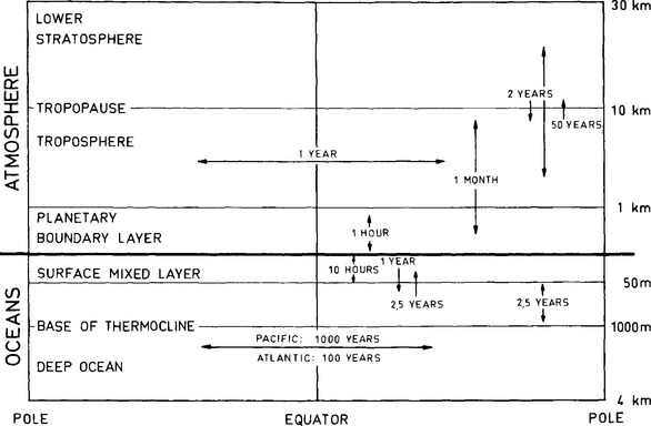
Some important time scales characterizing the transport within the oceanic and atmospheric environments are summarized in Fig. 4-17. In view of the somewhat ambiguous nature of the definitions of these time scales, the numbers should not be considered as more than indications of the magnitudes.
Acknowledgement.
I wish to thank Anders Björkström and Michael Jacobson for valuable comments on the manuscript.
Questions
4-1. Consider a reservoir with two separate sources Q1 and Q2 and a single sink S. The magnitudes of Q1 and S and their uncertainties have been estimated to be 75 ± 20 and 100 ± 30 (arbitrary units). Assuming that there is no direct way of estimating Q2, how would you derive its magnitude and uncertainty range from budget considerations? What assumption must be made regarding the reservoir?
4-2. Calculate the turnover time of carbon in the various reservoirs given in Fig. 4-3.
4-3. What is the relation between the turnover time τ0 the average transit time τr, and the average age τa, in a reservoir where all “particles” spend an equal time in the reservoir?
4-4. Consider a reservoir with a source flux Q and two sink fluxes S1 and S2. S1 and S2 are proportional to the reservoir content M with proportionality constants k1 and k2. The values of k1 and k2 are (1 yr−1) and (0.2 yr−1), respectively. The system is initially in steady state with M = M0 and Q = S10 + S20. Describe the change in time of M if the source is suddenly reduced to half its initial value. What is the response time of the reservoir?
4-5. Consider the water balance of a lake with a constant source flux Q. The outlet is the “threshold” type where the sink is proportional to the mass of water above a threshold value M1; S = k(M – M1). Calculate the turnover time of water at steady state and the response time relative to changes in Q.
4-6. For the more mathematically inclined: Investigate the dynamic behavior of a coupled linear three reservoir model using the technique outlined in Section 4.3.1. Answers can be found on p. 509.
SCOPE Report 29 Bolin, B. How much CO2 will remain in the atmosphere? In: Bolin B., Döös B. R., Jäger J., Warrick R. A., eds. The Greenhouse Effect, Climate Change, and Ecosystems. Sunderland, MA: Wiley, 1986.
Bolin, B., Rodhe, H. A note on the concepts of age distribution and transit time in natural reservoirs. Tellus. 1973; 25:58–62.
(short version) Braun, M. Differential Equations and their Applications, 3rd edn. Chichester: Springer-Verlag; 1983.
Chameides, W. L., Perdue, E. M. Biogeochemical Cycles. New York: Oxford University Press; 1997.
Eriksson, E. Compartment models and reservoir theory. Ann. Rev. Ecol. Syst. 1971; 2:67–84.
Feichter, J., Kjellström, E., Rodhe, H., Dentener, F., Lelieveld, J., Roelofs, G. -J. Simulation of the tropospheric sulfur cycle in a global climate model. Atmos. Environ. 1996; 30:1693–1707.
Follmi, K. B. The phosphorus cycle, phosphogenesis and marine phosphate-rich deposits. Earth Sci. Rev. 1996; 40:55–124.
Fox, J. L., Wofsy, S. C., McElroy, M. B., Prather, M. J. A stratospheric chemical instability. J. Geophys. Res. 1982; 87:11 126–11 132.
Grelle, A., Lindroth, A. Eddy-correlation system for long-term monitoring of fluxes of heat, water vapor and CO2. Global Change Biol. 1996; 2:297–307.
Hamrud, M. Residence time and spatial variability for gases in the atmosphere. Tellus. 1983; 35B:295–303.
Hartmann, D. J. Global Physical Climatology. New York and Oxford: Academic Press; 1994.
IPCC. Climate Change 1995, The Science of Climate Change. In: Intergovernmental Panel on Climate Change. San Diego: Cambridge University Press; 1996.
Jahnke, R. A. (2000). Current edition.
Junge, C. E. Residence time and variability of tropospheric gases. Tellus. 1974; 26:477–488.
Keeling, C. D., Bacastow, R. B. Impact of individual gases on climate. In: Energy and Climate. US National Research Council; 1977:72–95.
Ko, M. K. W., Sze, N. D., Weisenstein, D. K. The roles of dynamical and chemical processes in determining the stratospheric concentration of ozone in one-dimensional and two-dimensional models. J. Geophys. Res. 1989; 94:9889–9896.
Lasaga, A. C. The kinetic treatment of geochemical cycles. Geochim. Cosmochim. Acta. 1980; 44:815–828.
Lerman, A. Geochemical Processes; Water and Sediment Environments. Washington, DC: Wiley; 1979.
Lerman, A., Mackenzie, F. T., Garrels, R. M. Modeling of geochemical cycles: phosphorus as an example. Geol. Soc. Am. Mem. 1975; 142:205–218.
Liss, P. Gas transfer: experiments and geochemical implications. In: Liss P. S., Slinn W. G. N., eds. Air-Sea Exchange of Gases and Particles. New York: D. Reidel Publ. Co. ; 1983:241–298.
Liss, P. S., Slinn, W. G. N. Air-Sea Exchange of Gases and Particles. Dordrecht: D. Reidel; 1983.
Mackenzie, F. T., Ver, L. M., Sabine, C., Lane, M., Lerman, A., C, N, P, S global biogeochemical cycles and modeling of global changeWollast, et al, eds. Interactions of C, N, P and S Biogeochemical Cycles and Global Change. NATO ASI Series; Vol. 14. Springer-Verlag, Dordrecht, 1993.
McDuff, R. E., Morel, F. M. M. The geochemical control of seawater (Sillén revisited). Environ. Sci. Technol. 1980; 14:1182–1186.
Prigogine, I. Introduction to Thermodynamics of Irreversible Processes. Berlin: Wiley-Interscience; 1967.
Prinn, R., Cunnold, D., Simmonds, P., Alyea, F., Boldi, R., Crawford, A., Fraser, P., Gutzler, D., Hartley, D., Rosen, R., Rasmussen, R. Global average concentration and trend for hydroxyl radicals deduced from ALE/GAGE trichloroethane (methyl chloroform) data for 1978–1990. J. Geophys. Res. 1992; 97:2445–2461.
Redfield, A. C. On the proportions of organic derivatives in sea water and their relation to the composition of plankton. In: James Johnstone Memorial Volume. New York: Liverpool University Press; 1934:176–192.
Rodhe, H. Budgets and turnover times of atmospheric sulfur compounds. Atmos. Environ. 1978; 12:671–680.
Rodhe, H., Björkström, A. Some consequences of non-proportionality between fluxes and reservoir contents in natural systems. Tellus. 1979; 31:269–278.
Siegenthaler, U. Uptake of excess CO2 by an outcrop-diffusion model of the ocean. J. Geophys. Res. 1983; 88:3599–3608.
Slinn, W. G. N. Air-sea transfer of particles. In: Liss P. S., Slinn W. G. N., eds. Air-Sea Exchange of Gases and Particles. Liverpool, England: D. Reidel Publ. Co. ; 1983:299–405.
Southam, J. R., Hay, W. W. Dynamical formulations of Broecker’s model for marine cycles of biologically incorporated elements. Math. Geol. 1976; 8:511–527.
White, W. H. Does the photochemistry of the troposphere admit more than one steady state? Nature. 1984; 309:242–244.
Williams, G. R. The coupling of biogeochemical cycles of nutrients. Biogeochemistry. 1987; 4:61–75.


