The differential equations for the conservation laws require boundary conditions for proper solution. Specifically, the Navier-Stokes momentum equation (4.38) requires the specification of the velocity vector on all surfaces bounding the flow domain. For an external flow, one that is not contained by walls or surfaces at specified locations, the fluid’s velocity vector and the thermodynamic state must be specified on a closed distant surface.
Figure 4.20 Interface between two media for evaluation of boundary conditions. Here medium 2 is a fluid, and medium 1 is a solid or a second fluid that is immiscible with the fluid above it. Boundary conditions can be determined by evaluating the equations of motion in the small rectangular control volume shown and then letting l go to zero with the upper and lower square areas straddling the interface.
On a solid boundary or at the interface between two immiscible fluids, some of the necessary boundary conditions may be derived from the conservation laws by examining a small thin control volume that spans the interface. A suitable control volume is shown in Figure 4.20 for the interface separating medium 2 (a fluid) from medium 1 (a solid or a fluid immiscible with fluid 2). This control volume moves with the interface's velocity us. When necessary, us can be developed from a specification of the shape of the interface (see Section 8.2). Here +n and –n are the unit normal vectors pointing into medium 2 and medium 1, respectively. The square surfaces of the control volume have area dA, are locally parallel to the interface, and are separated from each other by a small distance l. The two tangent vectors to the surface are t′ and t″, and are chosen so that t′×t″=n. Application of the conservation laws to the rectangular volume ldA as l → 0, keeping the two square area elements in the two different media, produces five boundary conditions. As l → 0, all volume integrals → 0 and the surface integrals over the four rectangular side areas, which are proportional to l, tend to zero unless there is interfacial (surface) tension.
Conservation of Mass Boundary Condition
The mass conservation result, obtained from the Figure 4.20 control volume and (4.5) with b = us, is:
m˙s=ρ1(u1−us)·n=ρ2(u2−us)·n.
(4.90)
where m˙s is the surface mass flux per unit area. Importantly, only the normal component (us·n) of us enters this boundary condition formulation. Thus, us can be chosen with arbitrary or convenient tangential components, and this feature of (4.90) allows simplifications when curved moving interfaces are studied using Cartesian coordinates. If medium 1 is a fluid that is immiscible with fluid 2, then no mass flows across the boundary, m˙s=0, and (4.90) reduces to u1·n = us·n and u2·n = us·n. If medium 1 is a solid that is not dissolving, subliming, ablating, or otherwise emitting material at the interface, then u1 = us so m˙s is again zero, and the conservation of mass boundary condition reduces to u2·n = us·n. In addition, if the solid is stationary then u2·n = 0. In general, (4.90) must be used without simplification when there is mass-flow through a moving surface, as in the case of a moving shockwave observed from a stationary vantage point.
Constant Surface Tension Boundary Condition
Before proceeding to the conservation of momentum boundary condition, the effects of surface tension forces and their relationship to the geometry of the interface within the thin rectangular control volume shown in Figure 4.20 must be identified. Surface tension and interfacial tension arise because of the differences in attractive intermolecular forces at gas-liquid and liquid-liquid interfaces, respectively. For clarity, the following discussion emphasizes surface tension at gas-liquid interfaces; however, the results are equally applicable to interfacial tension at liquid-liquid interfaces.
In general, attractive intermolecular forces dominate in liquids, whereas repulsive forces dominate in gases. However, as a gas-liquid interface is approached from the liquid side, the attractive forces are not felt equally because there are many fewer liquid-phase molecules near the interface. Thus there tends to be an unbalanced attraction toward the interior of the liquid on the molecules near the gas-liquid boundary. This unbalanced attraction leads to surface tension and a pressure increment across a curved gas-liquid interface that must be properly accounted for when conserving fluid momentum. A somewhat more detailed description is provided in texts on physicochemical hydrodynamics. Two excellent sources are Probstein (1994, Chapter 10) and Levich (1962, Chapter VII).
The thermodynamic basis for surface tension starts from consideration of the Helmholtz free energy (per unit mass) f, defined by:
f=e−Ts,
where the notation is consistent with that used in Section 1.8. H. Lamb, in Hydrodynamics (1945, 6th Edition, p. 456) writes, “Since the condition of stable equilibrium is that the free energy be a minimum, the surface tends to contract as much as is consistent with the other conditions of the problem.” If the free energy is a minimum, then the system is in a state of stable equilibrium, and f is called the thermodynamic potential at constant volume (Fermi, 1956, Thermodynamics, p. 80). For a reversible isothermal change, the work done on the system increases the free energy f:
df=de−Tds−sdT,
where the last term is zero for an isothermal change. Then, from (1.24), df = −pdυ = work done on the system. (These relations suggest that surface tension decreases with increasing temperature.)
For an interface of area = A, separating two fluids of densities ρ1 and ρ2, with volumes V1 and V2, respectively, and with a surface tension coefficient σ (corresponding to free energy per unit area), the total (Helmholtz) free energy F of the system can be written as:
F=ρ1V1f1+ρ2V2f2+Aσ.
If σ > 0, then the two media (fluids) are immiscible and A will reach a local minimum value at equilibrium. On the other hand, if σ < 0, corresponding to surface compression, then the two fluids mix freely since the minimum free energy will occur when A has expanded to the point that the spacing between its folds reaches molecular dimensions and the two-fluid system has uniform composition.
When σ > 0, minimum interface area is achieved by pressure forces that cause fluid elements to move. These pressure forces are determined by σ and the local curvature of the interface. Consider the situation depicted in Figure 4.21 where the pressure above a curved interface is higher than that below it by an increment Δp, and the shape of the fluid interface is given by η(x,y,z) = z−h(x,y) = 0. Here σ is assumed constant. The influence of surface tension gradients on fluid boundary conditions is considered in the next subsection. (Flows driven by surface tension gradients are called Marangoni flows and are largely beyond the scope of this text.) The origin of coordinates and the direction of the z-axis are chosen so that h, ∂h/∂x, and ∂h/∂y are all zero at x = (0, 0, 0). Plus, the directions of the x- and y-axes are chosen so that the surface’s principal radii of curvature, R1 and R2, are found in the x-z and y-z planes, respectively. Thus, the surface’s shape is given by:
Figure 4.21 The curved surface shown is tangent to the x-y plane at the origin of coordinates. The pressure above the surface is Δp higher than the pressure below the surface, creating a downward force. Surface tension forces pull in the local direction of t×n, which is slightly upward, all around the curve C and thereby balance the downward pressure force.
η(x,y,z)=z−(x2/2R1)−(y2/2R2)=0
in the vicinity of the origin. A closed curve C is defined by the intersection of the curved surface and the plane z = ζ. The goal here is to determine how the pressure increment Δp depends on R1 and R2 when pressure and surface tension forces are balanced as the area enclosed by C approaches zero.
First, determine the net pressure force Fp on the surface A bounded by C. The unit normal n to the surface η is:
The minus sign appears here because greater pressure above the surface (positive Δp) must lead to a downward force and the vertical component of n is positive. The x- and y-components of Fp are zero because of the symmetry of the situation (odd integrand with even limits). The remaining double integration for the z-component of Fp produces:
(Fp)z=ez·Fp=−πΔp2R1ζ2R2ζ.
This result could have been anticipated from the given geometry; it is merely the negative of the pressure increment, –Δp, times the area of the curved surface projected onto the plane z=ζ,π2R1ζ2R2ζ.
The net surface tension force Fst on bounding curve C can be determined from the integral:
Fst=σ∮Ct×nds,
(4.92)
where ds=dx1+(dy/dx)2 is an arc length element of C, and t is the unit tangent to C so:
and dy/dx is found by differentiating the equation for C, ζ=(x2/2R1)−(y2/2R2), with ζ regarded as constant. On each element of C, the surface tension force acts perpendicular to t and tangent to the curved interface. This direction is given by t×n so the integrand in (4.92) is:
where the approximate equality holds when x/R1 and y/R2 ≪ 1 and the area enclosed by C approaches zero. The symmetry of the integration path will cause the x- and y-components of Fst to be zero, leaving:
where y has been eliminated from the integrand using the equation for C, and the factor of four appears because the integral shown only covers one-quarter of the path defined by C. An integration variable substitution in the form sinξ=x/2R1ζ allows the integral to be evaluated:
(Fst)z=ez·Fst=πσ2R1ζ2R2ζ(1R1+1R2).
For static equilibrium, Fp + Fst = 0, so the evaluated results of (4.91) and (4.92) require:
Δp=σ(1/R1+1/R2),
(1.11)
where the pressure is greater on the side of the surface with the centers of curvature of the interface. Thus, in the absence of buoyant forces and fluid motion, a bubble in water will assume a spherical shape since that shape minimizes its radii of curvature, or equivalently, its surface area (see Rayleigh 1890, or Batchelor 1967).
For air bubbles in water, gravity is an important factor for bubbles of millimeter size. The hydrostatic pressure in a liquid is obtained from pL = po – ρgz, where z is measured positively upwards from the free surface and gravity acts downwards and po is the pressure at z = 0. Thus, for a gas bubble beneath the free surface:
pG=pL+σ(1/R1+1/R2)=po−ρgz+σ(1/R1+1/R2).
Gravity and surface tension forces are of the same order over a length scale (σ/ρg)1/2. For an air bubble in water at 288 K, this length scale is: (σ/ρg)1/2 = [7.35 × 10⁻² N/m/(9.81 m/s2 × 103 kg/m3)]1/2 = 2.74 × 10⁻³ m. Analysis of surface tension effects results in the appearance of additional dimensionless parameters in which surface tension is compared with other effects such as viscous stresses, body forces such as gravity, and inertia. These are defined in Section 4.11.
Conservation of Momentum Boundary Conditions
Now return to the development of boundary conditions from Figure 4.20 and consider the normal direction. In this case, the momentum conservation result, obtained from (4.18) and (4.20b) with b = us, is:
where τij is the viscous stress tensor given by (4.59), and the tangent unit vectors t′ and t″ lie along the principal directions of interface curvature (with radii of curvature R′ and R″). This condition sets the normal velocity difference at an interface. When the both fluids are not moving, or when m˙s=0 and the fluids are inviscid, (4.93) reduces to (1.11).
Interestingly, a requirement on the tangential fluid velocity components at an interface cannot be developed from the equations of motion. Fortunately, the no-slip condition provides a simple experimentally verified result that addresses this analytical insufficiency. The simplest statement of the no-slip condition is that tangential velocity components must match at the interface:
u1·t′=u2·t′,andu1·t″=u2·t″.
(4.94a,b)
This condition has been under discussion for centuries, and kinetic theory does provide insights into its validity for gases. The no-slip condition is widely accepted as an experimental fact in macroscopic flows of ordinary fluids (Panton 2005, White 2006). For the simplest case of a viscous fluid (medium 2) moving with respect to an impermeable solid (medium 1), (4.90) and (4.94a,b) all together reduce to the interface condition:
u2=u1,
(4.95)
and this viscous-flow boundary condition is used throughout this text. Known violations of the no-slip boundary condition occur in rarefied gases and for superfluid helium at or below 2.17 K, where it has an immeasurably small (essentially zero) viscosity. Slip has also been observed in microscopic flows, and on micro-patterned and super-hydrophobic surfaces (Tretheway and Meinhart 2002, Gogte et al. 2005).
For the control volume in Figure 4.20, the tangential momentum conservation results from (4.18) and (4.94) are:
where τij is given by (4.59). These conditions include surface tension gradients and are statements of tangential stress matching at fluid-fluid interfaces. In general, (4.90), (4.93), (4.94), and (4.96) are required for analyzing multiphase flows with phase change.
Conservation of Energy Boundary Conditions
When the Figure 4.20 control volume is used with (4.48) and b = us, the following energy- conservation boundary condition can be developed:
m˙s[(h+12|u|2)2−(h+12|u|2)1]=−(k∇T)2·n+(k∇T)1·n.
(4.97)
When m˙s=0, the conductive heat flux must be continuous at the interface.
For a complete set of boundary conditions, the thermal equivalent of the no-slip condition is needed:
T1=T2
(4.98)
on the interface; no temperature jump is permitted. This condition is also widely accepted and is applied in the remainder of the text. However, it is known to be violated in rarefied gases and is related to viscous slip in such flows. Both topics are reviewed by McCormick (2005).
Example 4.15
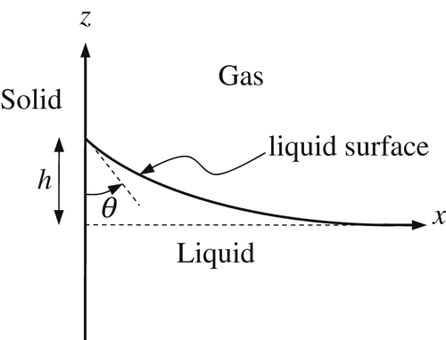
Calculate the shape of the free surface of a liquid adjoining an infinite vertical plane wall.
Solution
Here let z = ζ(x) define the free surface shape. With reference to Figure 4.22 where the y axis points into the page, 1/R1 = [∂2ζ/∂x2][1 + (∂ζ/∂x)2]–3/2, and 1/R2 = [∂2ζ/∂y2][1 + (∂ζ/∂y)2] –3/2 = 0. At the free surface, ρgζ−σ/R1 = const. As x → ∞, ζ → 0, and R2 → ∞, so const = 0. Then ρgζ/σ−ζ″/(1 + ζ′2)3/2 = 0.
Figure 4.22 Free surface of a liquid adjoining a vertical plane wall. Here the contact angle is θ and the liquid rises to z = h at the solid wall.
Multiply by the integrating factor ζ′ and integrate. We obtain (ρg/2σ)ζ2 + (1 + ζ′2)–1/2 = C. Evaluate C as x → ∞, ζ → 0, ζ′ → 0. Then C = 1. We look at x = 0, z = ζ(0) = h to find h. The slope at the wall, ζ′ = tan(θ + π/2) = −cotθ. Then 1 + ζ′2 = 1 + cot2θ = csc2θ. Thus we now have (ρg/2σ)h2 = 1 − 1/cscθ = 1 − sinθ, so that h2 = (2σ/ρg)(1 − sinθ). Finally we seek to integrate to obtain the shape of the interface. Squaring and rearranging the result above, the differential equation we must solve may be written as 1 + (dζ/dx)2 = [1 − (ρg/2σ)ζ2]–2. Solving for the slope and taking the negative square root (since the slope is negative for positive x):
dζ/dx=−{1−[1−(ρg/2σ)ζ2]2}1/2[1−(ρg/2σ)ζ2]−1.
Define σ/ρg = δ2, ζ/δ = γ. Rewriting the equation in terms of x/δ and γ, and separating variables:
2(1−γ2/2)γ−1(4−γ2)−1/2dγ=d(x/δ).
The integrand on the left is simplified by partial fractions and the constant of integration is evaluated at x = 0 when η = h/δ. Finally:

 and
and  , and are chosen so that
  . Application of the conservation laws to the rectangular volume ldA as l → 0, keeping the two square area elements in the two different media, produces five boundary conditions. As l → 0, all volume integrals → 0 and the surface integrals over the four rectangular side areas, which are proportional to l, tend to zero unless there is interfacial (surface) tension.