Equilibrium, Rate, and Natural Systems

5.1 Introduction

This chapter applies the physical chemistry taught in the first year of undergraduate chemistry to chemical problems in the natural environment and introduces key chemical concepts to use and keep in mind for the rest of this book. The material in this chapter is especially important to consider when utilizing the modeling techniques presented in Chapter 4.

There are two principal chemical concepts we will cover that are important for studying the natural environment. The first is thermodynamics, which describes whether a system is at equilibrium or if it can spontaneously change by undergoing chemical reaction. We review the main first principles and extend the discussion to electrochemistry. The second main concept is how fast chemical reactions take place if they start. This study of the rate of chemical change is called chemical kinetics. We examine selected natural systems in which the rate of change helps determine the state of the system. Finally, we briefly go over some natural examples where both thermodynamic and kinetic factors are important. This brief chapter cannot provide the depth of treatment found in a textbook fully devoted to these physical chemical subjects. Those who wish a more detailed discussion of these concepts might turn to one of the following texts: Atkins (1994), Levine (1995), Alberty and Silbey (1997).

In many cases one can apply the first principles of thermodynamics and chemical kinetics to natural systems only with caution. The reason has little to do with the shortcomings of the core chemical principles. Rather, the application of thermodynamics (including electrochemistry) can be restricted by the fact that some natural systems have reaction rates so slow that they exist for long periods under non-equilibrium conditions. Moreover, reaction rates can be difficult to characterize when they are sensitive to poorly understood catalytic (including enzymatic) effects or to surface effects. Applications of thermodynamics and kinetics, as they are presented in this chapter, require knowledge of many variables such as concentration, temperature, and pressure. However, in contrast to reactions in a stirred beaker, the natural world may have large gradients of these variables. The natural environment also differs because of the large number of chemical species that coexist and interact concurrently. Therefore, it is important that the limitations of chemical thermodynamics and kinetics be considered before they are applied to biogeochemical systems.

5.2 Thermodynamics

5.2.1 State Functions and Equilibrium Constraints

The laws of thermodynamics are the cornerstones of any description of a system at equilibrium. The First Law, also known as the Law of Conservation of Energy states that energy cannot be created or destroyed, i.e., the energy of the universe is constant. Thus if the internal energy of a system decreases in a reaction, the chemical change is accompanied by a release of energy, often in the form of heat. The enthalpy, H, is a property of the system that is equal to E+PV, where E is the internal energy of the system, P is pressure, and V is volume. At constant pressure, the change in H is the energy flow as heat. Enthalpy is a state function of the system, which means that it is a property that depends only on the state of the system and not how it managed to arrive at that state. Other state functions are temperature and pressure. Work and heat are examples of properties that are not state functions.

The Second Law of thermodynamics states that for a chemical process to be spontaneous, there must be an increase in entropy. Entropy (S) can be thought of as a measure of disorder.

Another property of the system, G, the free energy, or the Gibbs free energy, is related to enthalpy and entropy by:

(1)

When the temperature of reactants and products are equal, ΔG is given by

(2)

The second law also describes the equilibrium state of a system as one of maximum entropy and minimum free energy. For a system at constant temperature and pressure the equilibrium condition requires that the change in free energy is zero:

(3)

We represent a change in a quantity for any chemical reaction as the value of that quantity for the products of the reaction minus the value of that quantity for reactants. It is important to keep in mind that the terms reactant and product refer only to how the chemical equation is written and not to whether or not the substance is actually being formed or is disappearing.

Equation (3) defines the equilibrium condition under the constraint that temperature and pressure are constant. A related consequence of the Second Law is that if ΔG < 0 the reaction of the reactant to product is thermodynamically spontaneous. Thermodynamic spontaneity means that the system has the potential to react. The more negative ΔG, the more spontaneous the reaction. The actual time scale for the reaction to occur can vary greatly. A good example of a non-equilibrium system is the ambient pressure of nitrogen oxides in the troposphere, which can greatly exceed their equilibrium values for the equilibrium with N₂ and O₂. We discuss non-equilibrium systems later in the chapter.

Although ΔG is the overall determinant of spontaneity, it is convenient to examine the two thermodynamic components of ΔG. The ΔH term is largely a function of the strengths of the chemical bonds in reactant and product. To the extent that there are more strong bonds (and strong associations between molecules) in the product than in the reactant, ΔH will be negative. An examination of Equation (3) shows that a negative ΔH contributes to the overall spontaneity of the reaction.

The ΔS term is a measure of the relative degree of disorder in reactant and product. To the extent that the product has greater disorder than the reactant ΔS will be positive. A positive ΔS will contribute to the overall spontaneity of the reaction. ΔS for a reaction can be evaluated from tables of entropy data. Moreover, the sign of ΔS for gas phase reactions may often be determined without entropy tables. For gas phase systems in which the number of independent molecules and atoms is greater in the product, ΔS will be positive. If there is no change in the number of atoms and molecules for a gas phase reaction it is difficult to say (without evaluating AS from tables of data) whether AS is positive or negative. In the liquid phase these simple rules for AS are less easily applied because significant entropy effects occur in water and many other solvents. Ionic solutes can cause a relative lowering of entropy of the solution by forming highly ordered associations with water, whereas other solutes may increase the solution entropy by disrupting the structure of water and not replacing it with other low-entropy structures.

In practice, G and H for a substance are defined relative to the G and H for the constituent elements of that substance. These relative values are known as free energy of formation and enthalpy of formation for standard conditions and symbolized as ΔG⁰ and ΔH⁰. So where we indicated values of G and H in Equations (1) and (2), in practice we would use a free energy and enthalpy of formation, which are themselves a special kind of ΔG and ΔH. Values for these functions may be obtained from standard tables of thermodynamic data, usually for the reference temperature of 298.2 K and a pressure of 1.0 bar. The Chemical Rubber Company handbook (Lide, 1998) is one of the more commonly available sources.

More complete sources, including some with data for a range of temperatures, are listed in the references at the end of the chapter. Note that many tabulations (including many contemporary biological sources) still represent these energy functions in calories and that it may be necessary to make the conversion to joules (1 cal = 4.1840 J). Because of the definition of the energy of formation, elements in their standard state (carbon as graphite, chlorine as Cl₂ gas at one bar, bromine as Br₂ liquid, etc.) have free energies and enthalpies of formation equal to zero. If needed, the absolute entropies of substances (from which AS may be evaluated) are also available in standard sources.

For ions in the aqueous phase there is an additional complication in defining G and H. The change in G and H for the formation of an ion from its constituent element (e.g. 1/2 Cl₂(g) + e⁻ → Cl⁻(aq)) is defined relative to the change in G and H for the formation of H⁺ from H₂(g). This relative change in G and H is termed the standard free energy or enthalpy of formation for ions. As a result of this definition, ΔG⁰ and ΔH⁰ for the formation of H⁺ are zero. In practice, the definitions given above lead to the following algorithm for determining ΔG⁰ or ΔH⁰ for a reaction. ΔG⁰ for a reaction may be obtained by simply adding the ΔG⁰ (formation) values for the product species and subtracting the sum of ΔG⁰ (formation) for all reactant species. Where an element in its standard state or H⁺ is involved, substitute zero.

5.2.2 Gas Phase Equilibria

For reactions in the gas phase, the free energy per mole of gas as a function of pressure is given by the following expression:

(4)

where P⁰ is the standard reference pressure (commonly 1 bar or (1/1.01325) atmosphere), and P is the pressure of the gas, R is the universal gas constant, which has a value of 8.314 J/mol/K, and T is the temperature of the system in kelvins (°C + 273). For the ideal systems considered here, we will treat the free energy per mole to be the same as the chemical potential. This treatment works best at very low pressures where gases approach ideal behavior.

For the gas phase equilibrium

the change in free energy for this system at equilibrium is

substituting the expression for G⁰ given in Equation (4), we derive the familiar equilibrium constant expression:

(5)

We will see functions like the one occurring under the logarithm operator quite often. For efficiency, this is generally written as ln(Products)/(Reactants), where (Products) and (Reactants) denote the partial pressures of the species relative to the standard state pressure raised to a power that is equal to the stoichiometric coefficients. K_P is the equilibrium constant in terms of pressures. Since all pressures are in the same units, K_P is dimensionless. Note that in some literature there may be a combination of some power of P⁰ with K_P to obtain an equilibrium constant with pressure units. In this case,

Although K_p for a gas phase reaction is defined in terms of the partial pressures of reactants and products, at times it is more convenient to express the equilibrium constant for an equilibrium system in terms of moles or molecules per unit volume. The equilibrium constant in concentration terms is related to K_p by using the ideal gas equation by the following conversion:

(6)

where K_c is the equilibrium constant in mole/volume units, and An is the change in the number of moles of gas for the reaction. In the case of the NO₂ equilibrium, Δn = –1.

5.2.3 Condensed Phase Equilibria

For reactions involving a nearly pure liquid or solid (often the case for water in aqueous solutions) G is given by the following expression, where X is the mole fraction of the liquid:

(7)

However, for reactions occurring in dilute solutions, we use the following expression:

(8)

which is parallel to the expression given for gases in Equation (4). Here c is the concentration of the solute (usually in units of moles per liter), and c⁰ is the concentration in the standard state (defined as exactly 1 molar (M)). The ratio c/c⁰ is related to the activity (for ideal solutions), which is defined by

(9)

The activity is a measure of the tendency of a substance to react relative to its reacting tendency in the standard state. Here we relate activity to c/c⁰ for ideal solutions. For ideal gases and ideal solvents, the activity approaches P/P⁰ and X, respectively. Although c⁰ is taken to be 1.0 M, Equation (8) works best when c is much less than 1.0 M.

One may combine the appropriate expressions for G for equilibria involving reactants in different phases to obtain a general expression, which relates the equilibrium constant to the change in free energy:

(10)

Here K_eq may be a mixed expression involving pressures, mole fractions, and molar concentrations.

The van′t Hoff equation describes the temperature dependence of the equilibrium constant.

(11)

Thus the degree of spontaneity at a given temperature depends on ΔG⁰, but the change in spontaneity (as defined by the equilibrium constant) with temperature is given by Equation (11) and depends only on ΔH⁰. If the change in temperature is small, one may assume that ΔH° is constant and integrate Equation (11) directly. For larger ranges in temperature one will need to know something about the temperature dependence of ΔH⁰. This depends on the heat capacities of reactants and products.

5.2.4 Mixed Phases

As mentioned after Equation (10), the equilibrium constant may be expressed when the reactants are in several phases. As an example, the equilibrium between ammonia in a large cloud droplet and in the gas phase, NH₃(aq) and NH₃(g), is described by the equilibrium constant expression

Here c_NH₃ is the concentration of undissociated ammonia in water. The equilibrium constant for this class of equilibria is often defined in terms of a Henry’s Law constant, K_H.

The ΔG⁰ value for NH₃(aq) should be for dilute aqueous solutions. Note that K_H has units.

The solubility equilibrium for CaCO₃ (calcite) ↔ Ca²⁺(aq) +⁻ (aq) is defined by

where K_SP stands for Solubility Product. This equilibrium constant does not contain a term for CaCO₃ (calcite). To the extent that the calcite is a pure solid (does not contain dissolved impurities) and consists of particles large enough that surface effects are unimportant, this equilibrium does not depend on the “concentration” of calcite or particle size. Exceptions to this case are important in the formation of cloud droplets (where the particle size dependence is known as the Kelvin effect), which is discussed in Chapter 7, and in the solubility of finely divided solids.

5.2.5 Aggregate Variables

A knowledge of the concentrations of all reactants and products is necessary for a description of the equilibrium state. However, calculation of the concentrations can be a complex task because many compounds may be linked by chemical reactions. Changes in a variable such as pH or oxidation potential or light intensity can cause large shifts in the concentrations of these linked species. Aggregate variables may provide a means of simplifying the description of these complex systems. Here we look at two cases that involve acid-base reactions.

Al(III) is an example of an aquatic ion that forms a series of hydrated and protonated species. These include AlOH²⁺,, Al(OH)₃, and other forms in addition to Al³⁺. (For simplicity, we omit the H₂O molecules that complete the structures of these complexes.) Most of these species are amphoteric (able to act as an acid or a base). Thus the speciation of Al(III) and many other aquatic ions is sensitive to pH. In this case, an aggregate variable springs from the conservation of mass condition. In the case of dissolved aluminum, the total dissolved aluminum is given by

For many problems Al_T is a constant or is known. The above condition thus constrains the concentrations of the individual species. A similar case occurs in carbonate equilibria, which leads to the formation of H₂CO₃,, and Total dissolved carbon is represented by

In the case of CO₂ one must consider the hydrated form (H₂CO₃) and the non-hydrated form, CO₂(aq). This latter form is in equilibrium with the atmosphere:

The CO₂(aq) is in turn in equilibrium with H₂CO₃(aq):

for which K_eq ≈ 650. For many purposes, CO₂(aq) and H₂CO₃ are lumped together as “carbonic acid,” or H₂. The Henry’s Law and acid-base equilibria are often written in terms of H₂ (Stumm and Morgan, 1981). Given the value of K_eq, most “carbonic acid” is in fact CO₂(aq).

Alkalinity is helpful in describing the acid-neutralizing ability of an aqueous solution that may contain many ions. In any ionic equilibrium there is a conservation of charge condition.

We may further break this down to

(12)

Conservative ions are ones that do not undergo acid-base reactions at the pH values of interest. These include Na⁺, K⁺, Ca²⁺,, Cl⁻, etc. Non-conservative ions do undergo acid base reactions. These include H₃O⁺, OH⁻,,

and Alkalinity is defined as follows.

(13)

If, for example, we make a 0.10 M solution of KOH, the only conservative ions would be K⁺ at 0.10 M and the alkalinity would be 0.10 M. The alkalinity would be – 0.10 M for a 0.10 M solution of HCl. Negative alkalinity is also known as acidity.

Solutions to complex ionic equilibrium problems may be obtained by a graphical log concentration method first used by Sillén (1959) and more recently described by Butler (1964) and Morel (1983). These types of problems are described further in Chapter 16 as they relate to natural systems. Computer-based numerical methods are also used to solve these problems (Morel, 1983).

5.2.6 Conditions Far-Removed from Standard Conditions

For many cases one needs to have values of thermodynamic variables for conditions very different from 298 K and 1.0 bar. These cases include reactions occurring above the tropopause, where pressures are several orders of magnitude less than 1.0 bar and temperatures are less than 200 K. The important reactions occurring in the high-temperature and high-pressure aqueous conditions of the mid-ocean rift zone, and the high-temperature and high-pressure conditions where important mineral transformations occur far below the Earth’s surface are examples.

We offer two approaches for obtaining ΔH and ΔG values for these conditions. In the most straightforward approach, the functions (G – H)/T and (H – H₂₉₈)/T, are tabulated for extensive temperature ranges for many simple molecules. The advantage of these functions is that they change in a very regular manner with respect to temperature and thus can easily be interpolated from tables. Once one has a value for these functions for a given T, then calculating ΔG_T or ΔH_T is straightforward.

The second approach to getting data relies on basic thermodynamic relationships between G and H, and T and P. For instance, the heat capacity at constant pressure (C_p) of a substance is defined by:

(14)

From this definition, we can obtain an expression for the temperature dependence of ΔH of a reaction, if the heat capacity at constant pressure is known. For the pressure dependence, the following fundamental relationship offers a good start:

(15)

where α is the coefficient of thermal expansion:

(16)

Thus, in this approach one will need tables (or functions) for C_p, α, and possibly the compressibility as functions of T and P for the substances in question.

5.2.7 Non-ideal Behavior

Departures from ideality have been studied extensively for gases and gas mixtures. For most conditions of interest in the Earth’s atmosphere, the assumption of ideal behavior is a reasonable approximation. The two most prevalent gases (N₂ and O₂) are non-polar and have critical temperatures (126 K and 154 K) far below most temperatures of environmental interest. These gases behave fairly ideally even though their pressures are high. For other gases, the partial pressures common in the atmosphere are so low that ideal behavior is a good approximation.

Departures from ideality are much more common in the condensed phase. A significant departure from ideality results from the effect of the ionic strength of aqueous solutions on the energies of ions. This effect should be considered in any quantitative consideration of ionic equilibria in sea water (Stumm and Morgan, 1981).

5.2.8 Thermodynamic Description of Isotope Effects

Thermodynamic energy terms (and equilibrium constants) may differ for compounds containing different isotopic species of an element. This effect is described in theoretical detail by Urey (1947), and applications to geochemistry are discussed by Broecker and Oversby (1971) and Faure (1977). A good example is the case of the vapor/liquid equilibrium for water. The vapor pressure of a lighter isotopic species, ¹O, is higher relative to that of heavier species, ¹H²H¹⁶O (or HD¹⁶O), ¹O, and others.

Small variations in isotopic composition are usually described by comparing the ratio of isotopes in the sample material to the ratio of isotopes in a reference material. The standard measure of isotopic composition is δX ′ defined in parts per thousand (per mil or %) by

(17)

The amounts of the standard isotopic species and the tracer isotopic species are represented by X and X’ for the sample and the reference material. The reference substance is chosen arbitrarily, but is a substance that is homogeneous, available in reasonably large amounts, and measurable using standard analytical techniques for measuring isotopes (generally mass spectrometry). For instance, a sample of ocean water known as Standard Mean Ocean Water (SMOW) is used as a reference for ²H and ¹⁸O. Calcium carbonate from the Peedee sedimentary formation in North Carolina, USA (PDB) is used for ¹³C. More information about using carbon isotopes is presented in Chapter 11.

If the sample has less of the tracer isotopic species than the reference material, δ is negative. Since many of the tracer species are heavier than the reference species (e.g., ¹⁴C and ¹³C vs. ¹²C or ³⁴S vs. ³²S), substances having less of a tracer species than the standard species are said to be “light.”

As an example, the ratio of the equilibrium vapor pressures for ¹⁶O water, P₁₆ and ¹⁸O water, P₁₈, depends on temperature and is expressed by the following equation, derived from Faure (1977) (temperature is in kelvins):

(18)

At 25°C the ratio of equilibrium pressures is 1.0088 (from the above equation). This means that pureO has a slightly greater vapor pressure than pureO. The ratio of ¹⁸O to ¹⁶O in the atmosphere is equal to the ratio in the ocean times 1/1.0088.

Water vapor formed at low latitudes by evaporation from the ocean is “lighter” than the ocean water from which it evaporated. As this water moves to higher latitudes and the first bit of vapor condenses and rains out, the rain is heavier than the vapor from which it forms, and the removal by rain makes the vapor remaining in the atmosphere even lighter. Further precipitation at still higher latitudes makes δ¹⁸O for the remaining vapor even more negative. Precipitation at high latitudes is thus lighter than low-latitude precipitation.

As may be seen from the equation given above, the degree of fractionation of water increases as temperature decreases. δ¹⁸O in ice cores from Greenland and Antarctica is more negative for those periods in which evaporation leading to precipitation occurred at a lower temperature. Measurements of δ¹⁸O and δ²H can thus be used as a means of tracking changes in mean temperatures (Faure, 1977; Saigne and Legrande, 1987). This and other information derived from ice cores is presented in Chapter 18. The kinetic basis for the isotope effect is discussed later in this chapter.

5.3 Oxidation and Reduction

Reactions in which electrons are transferred from one reactant to another (oxidation-reduction or redox reactions) are a subset of systems described by thermodynamics. We focus on the transfer of electrons when examining conditions for spontaneity and equilibrium for oxidation reduction systems because the electrons are a common currency for comparing many different reactions. The potential for electrons to be transferred in one direction or another reflects the thermodynamic spontaneity of the reaction.

5.3.1 Half-Cell Conventions and the Nernst Equation

The elemental reaction used to describe a redox reaction is the half reaction, usually written as a reduction, as in the following case for the reduction of oxygen atoms in O₂ (oxidation state 0) to H₂O (oxidation state –2). The half-cell potential, E⁰, is given in volts after the reaction:

E⁰ represents the relative tendency for this reaction to occur. This can also be thought of as the driving force for the reaction. The half-cell free energy change, ΔG⁰ is a related quantity that gives the free energy change for the given reaction at standard conditions relative to the reduction for the standard hydrogen electrode, for which the half reaction is

The half-cell potential and the half-cell free energy change are related by the following relationship for reversible conditions:

(19)

where F is the Faraday constant (=94 490 C/mol or 94 490 J/V/mol) and z is the number of electrons appearing in the balanced reduction half cell. A negative value for ΔG⁰ (or a positive value for E⁰) means that the given reduction has a greater tendency to occur than does the reduction of H⁺ to H₂. ΔG⁰ values are easily obtained from tables of thermodynamic data. As mentioned above, ΔG⁰ is zero by convention for elements in their standard states and for H⁺.

The Nernst equation describes the dependence of the half-cell potential on concentration:

(20)

The function [Products]/[Reactants] is the same as defined in Sections 5.2.2 and 5.2.3. The factor 2.303RT/F has the value 0.05916 at the common reference temperature of 298.2 K. The factor 2.303 results from the change from a natural logarithm (used to express the concentration dependence of thermodynamic functions) to the common logarithm (more often used in electrochemistry and in measurements of hydrogen ion activity). The symbolism E_h, is often used to make clear that we are representing a half-cell potential relative to the standard hydrogen electrode. Since E⁰ is listed above to be 1.2290 V for the reduction of oxygen, then assuming that the water is pure, the Nernst equation for reduction of oxygen comes out to be

(21)

5.3.2 Electron Activity and pε

As an alternative, the tendency for a reduction to occur may also be expressed in terms of a hypothetical electron activity based on the standard hydrogen electrode. Activity was functionally defined in Equation (9). The free energy of an electron is related to chemical activity of the electron by

(22)

where a_e is electron activity. The free energy change for a process in which z electrons move from a standard hydrogen electrode to some other electrode is therefore

(23)

where a_SHE is the standard hydrogen electrode electron activity.

We connected our earlier definition of activity to a standard state of 1.0 bar or 1.0 M or a mole fraction of unity. None of these make much sense for electrons, but we may define electron activity in terms of the standard hydrogen electrode. We define a_SHE to be unity, and we define a term related to electron activity, pε:

(24)

Hostettler (1984) discusses issues involved in associating pε with electron activity.

One of the conditions of spontaneity is that ΔG < 0 at constant T and P. A new statement of this condition is that in a spontaneous process electrons (or any other substance) move from a state of higher activity to a state of lower activity. Because of the definition of pε as a negative logarithm of activity, the condition of spontaneity for pε is that electrons move from a more negative to a more positive pε.

We can combine the definition of pε with the Nernst equation to obtain a relationship between pε and concentrations:

(25)

5.3.3 pε/pH Stability Diagrams

We can write pε expressions for the reduction of O₂ to H₂O and the reduction of H⁺ to H₂. For the reaction

If we use the relationship between pε⁰ and E⁰ implied by Equation (22) and assume an oxygen pressure of 1.0 bar, then

For the reduction of H⁺ at a hydrogen pressure of 1.0 bar,

We draw two lines representing these two expressions for pε as a function of pH in Fig. 5-1. We discuss five cases for this system:

Fig. 5-1 Stability diagram for H₂O.

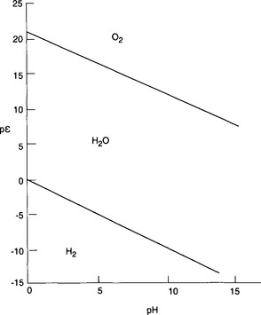
Case 1. Along the lower line H₂ and H⁺ are in equilibrium when pε = –pH.

Case 2. If p ε < −pH (perhaps as the result of an applied voltage or the presence of another electrode), the electrons will have a greater activity than those in equilibrium with a standard hydrogen electrode, and H⁺ will be reduced to H₂. This is the stability region for H₂.

Case 3. Along the upper line O₂ (at 1.0 bar) and H₂O are in equilibrium.

Case 4. Above the upper line, pε > +20.77 – pH and O₂ is stable.

Case 5. If pε lies between the two lines, H₂O is stable.

Consider for a moment what happens if we provide a path for electron flow between the O₂/H₂O electrode and the H⁺/H₂O electrode. The activity of electrons in equilibrium with the O₂/H₂O electrode is 10^−20.77 that of electrons associated with H⁺/H₂O. Electrons will flow from the H⁺/H₂O electrode to the O₂/H₂O electrode.

As a more complex example, we examine the stability of oxidation states of aqueous sulfur as a function of pH. This exercise will bring out the treatment of thermodynamically unstable species and the change of sulfur speciation with pH.

The sulfur species include those in the +6 oxidation state (or S(VI)) and also S(IV), S(0), and S(–II). The necessary reduction reactions are

Some of the thermodynamic data and equilibrium constants that are required follow.

Free energies of formation:

• H₂O(liq), – 237.18 kJ/mol.

• (aq), – 744.6 kJ/mol.

• (aq), – 486.6 kJ/mol.

• S²⁻ (aq), +85.8 kJ/mol.

Acidity constants:

• H₂SO₄, pK₁₁ ∼ –3, pK₁₂ = 1.9.

• H₂SO₃, pK₂₁ = 1.8, pK₂₂ = 7.2.

• H₂S, pK₃₁ = 7.1, pK₃₂ = 14.

We could write many more reactions involving these species, but, as will be seen, the ones above are sufficient. We will also assume a total sulfur concentration of 0.010 M, but we need to know how pH affects the distribution of sulfur-containing acids and bases. For any acid

which we rearrange to

Looking at the second form of this equation, if [H⁺] K_A, then [HA] [A⁻]. Essentially all of the “A” species is present as HA under these conditions. When [H⁺] K_A, practically all of the “A” species are present as A⁻.

We summarize below what this means for our sulfur species:

• S(VI) –3 <pH <1.9, is the dominant species;

pH >1.9, is the dominant species.

• S(IV) pH < 1.8, H₂SO₃ is dominant;

1.8 < pH <7.2, is dominant;

pH >7.2, is dominant;

• S(–II) pH < 7.1, H₂S is dominant;

7.1 < pH < 14, HS⁻ is dominant;

pH > 14, S²⁻ is dominant.

We next write the expression for pε for each of our three reactions:

In this section we will develop many different expressions for pε. At any given pH, only two or three of these equations will be relevant. We can begin by examining pε at any pH value, but let us begin at pH = 0. The dominant sulfur species at this pH are, H₂SO₃, and H₂S. We express the sulfur concentrations in terms of these dominant ions by making the following substitutions:

Using these substitutions with the numerical values for the constants, we obtain:

• for S(VI)/S(IV),

• for S(IV)/S(0),

• for S(0)/S(–II),

These pε values actually represent electron activities for a new set of half-cell reactions derived from reactions 1, 2, and 3:

1. + 3H⁺ + 2e⁻ → H₂SO₃ + H₂O

2. H₂SO₃ + 4H⁺ + 4e⁻ → S⁰ + 3H₂O

3. S⁰ + 2H⁺ + 2e⁻ → H₂S

The first thing to notice here is that pε₂>pε₁ for all pH values and concentrations of interest to us. Given the role of S(IV) in these two half cells, this means that H₂SO₃ in reaction 1 can always give up electrons to H₂SO₃ in reaction 2. The overall reaction in this case is

This is known as an autoredox reaction. S(IV) is thus not thermodynamically stable at all and need not be considered further in this problem. Instead of considering reactions 1 and 2, we consider the direction reduction of S(VI) to S(0),

The relevant equations are those for pε₃ above and the following for pε₄:

At pH near zero, this expression is

We can now start to draw a figure representing pε as a function of pH, as shown in Fig. 5-2.

Fig. 5-2 Working diagram for sulfur.

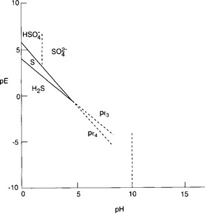
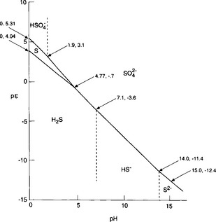
If pε lies below the pε₃ line then only H₂S is stable; for pε values between the pε₃ line and the pε₄ line, S⁰ is stable; for pε lying above the pε₄ line, is stable. At a pH of 1.9, the dominant S(VI) species changes to. The slope of the pε₄ curve changes slightly at pH = 1.9 reflecting a change in the number of protons in the balanced reaction:

The lines for pε₃ and pε₄ cross at a pH of about 4.77. For pH>4.77, pε₃>pε₄ and S(0) is no longer thermodynamically stable. S(0) will undergo an autoredox reaction to form S(VI) and S(–II). The only sulfur half cell between stable species is for the reduction of S(VI) to S(–II):

For the pH region from 4.77 to 7.1, this becomes

For 7.1 <pH <14, this expression becomes

For the case in which [HS⁻] and [] are equal, we have

We present the pε/pH diagram for the sulfur system in Fig. 5-3, which represents the sulfur system for a total sulfur concentration of 0.010 M. Note that as sulfur concentration decreases, the curve for pε₃ will displace upward and the curve for pε₄ will displace downward. The stability region for S(0) will be decreased and may even vanish.

Fig. 5-3 Stability diagram for sulfur.

5.3.4 Natural Systems and the Nernst Equation

The extent to which natural systems are described by the Nernst equation depends on the relative rates at which electrons are transferred to and from various substances. These rates vary over several orders of magnitude. For example, the reduction of the hydrated ferric ion,

may be a far simpler process then the reduction of nitrate,

The latter reaction must involve a large number of molecular steps and may be a much slower process. The mechanisms of a few inorganic electron transfer processes have been summarized by Taube (1968). The presence of very slow reactions when several redox couples are possible means that the E_h value measured with an instrument may not be related in a simple way to the concentrations of species present, and different redox couples may not be in equilibrium with one another. Lindberg and Runnells (1984) have presented data on the extent of disequilibrium in ground waters. Bockris and Reddy (1970), Stumm and Morgan (1981), and Hostettler (1984) describe factors that determine the potential of non-equilibrium redox systems.

5.4 Chemical Kinetics

5.4.1 Reaction Rates

As described in the first part of this chapter, chemical thermodynamics can be used to predict whether a reaction will proceed spontaneously. However, thermodynamics does not provide any insight into how fast this reaction will proceed. This is an important consideration since time scales for spontaneous reactions can vary from nanoseconds to years. Chemical kinetics provides information on reaction rates that thermodynamics cannot. Used in concert, thermodynamics and kinetics can provide valuable insight into the chemical reactions involved in global biogeochemical cycles.

In chemical kinetics an empirical relationship is used to relate the overall rate of a process to the concentrations of various reactants. A common form for this expression is

This equation is known as the rate law for the reaction. The concentration of a reactant is described by A; dA/dt is the rate of change of A. The units of the rate constant, represented by k, depend on the units of the concentrations and on the values of m, n, and p. The parameters m, n, and p represent the order of the reaction with respect to A, B, and C, respectively. The exponents do not have to be integers in an empirical rate law. The order of the overall reaction is the sum of the exponents (m, n, and p) in the rate law. For non-reversible first-order reactions the scale time, tau, which was introduced in Chapter 4, is simply 1/k. The scale time for second- and third-order reactions is a bit more difficult to assess in general terms because, among other reasons, it depends on what reactant is considered.

It is important to stress that the empirical rate law must be determined experimentally, with laboratory measurements of the rate constant and the coefficients m, n and p. A wide variety of laboratory experimental methods are used to determine these rate parameters. Further details on atmospheric and photochemical systems may be found in Calvert and Pitts (1966), Finlayson-Pitts and Pitts (1986), Seinfeld (1986) and Wayne (1985).

The temperature dependence of a rate is often described by the temperature dependence of the rate constant, k. This dependence is often represented by the Arrhenius equation, k=A exp(–E_a/RT). For some reactions, the temperature relationship is instead written k=ATⁿ exp(–E_a/RT). The A term is the frequency factor for the reaction, which reflects the number of effective collisions producing a reaction. E_a is known as the activation energy for the reaction, and is a measure of the amount of energy input required to start a reaction (see also Benson, 1960; Moore and Pearson, 1981).

Rate constants for a large number of atmospheric reactions have been tabulated by Baulch et al. (1982, 1984) and Atkinson and Lloyd (1984). Reactions for the atmosphere as a whole and for cases involving aquatic systems, soils, and surface systems are often parameterized by the methods of Chapter 4. That is, the rate is taken to be a linear function or a power of some limiting reactant – often the compound of interest. As an example, the global uptake of CO₂ by photosynthesis is often represented in the empirical form d[CO₂]/dt = –k[CO₂]^m. Rates of reactions on solid surfaces tend to be much more complicated than gas phase reactions, but have been examined in selected cases for solids suspended in air, water, or in sediments.

5.4.2 Molecular Processes

Rather than always occurring in one step, reactions in the natural world often result from a series of simple processes between atoms and molecules resulting in a set of intermediate steps from reactants to products. The way multistep reactions occur can have a strong effect on the kinetics of the overall reaction. For instance, in the formation of NO from N₂ and O₂, the direct process in which a molecule of N₂ collides with a molecule of O₂ to produce two molecules of NO is extremely slow relative to other pathways for producing NO. Instead, the formation of NO at the high temperatures present during combustion and lightning, is thought to result from a multistep reaction known as the Zeldovich mechanism (Bagg, 1971), where M may be any of several molecules:

A reaction mechanism is a series of simple molecular processes, such as the Zeldovich mechanism, that lead to the formation of the product. As with the empirical rate law, the reaction mechanism must be determined experimentally. The process of assembling individual molecular steps to describe complex reactions has probably enjoyed its greatest success for gas phase reactions in the atmosphere. In the condensed phase, molecules spend a substantial fraction of the time in association with other molecules and it has proved difficult to characterize these associations. Once the mechanism is known, however, the rate law can be determined directly from the chemical equations for the individual molecular steps. Several examples are given below.

Three basic types of fundamental processes are recognized: unimolecular, bimolecular and termolecular. Unimolecular processes are reactions involving only one reactant molecule. Radioactive decay is an example of a unimolecular process:

The rates of this process depend only on the concentration of reactant and the rate constant, which is generally temperature dependent.

The unit of the rate constant for a unimolecular process is 1/s.

Photolytic reactions such as the decomposition of ozone by light are also unimolecular processes:

The rate of this photolytic reaction is given by

Rate constants for photolytic reactions are commonly represented by the symbol J (unit 1/s). The first-order photolytic rate constant can be calculated using the formula:

The empirically determined absorption cross-section, σ(λ,T) in units of cm²/molecule, is a measure of the ability of a molecule to absorb light of a particular wavelength at a given temperature. The photon flux, I(λ) in units of photons/cm s nm), represents the number of photons of a certain wavelength range arriving at a 1 cm² area per second. Therefore, I(λ) and hence J increase with altitude, vary with time of day, and decrease to zero at night. The dimensionless quantum yield, ϕ(λ,T), describes the fraction of absorbed photons that results in the photolysis pathway of interest. For instance, O₃ can photolyze along several pathways including

O(³P) and O(¹D) represent different electronic states of the oxygen atom. The quantum yield for O(¹D) production, ϕ_O(¹D)(λ,T), is the fraction of photons of wavelength λ absorbed by ozone at temperature T that result in the formation of the excited O(¹D) atoms. Since photolysis can occur over a range of wavelengths, J is calculated over the integral from the shortest, λ₁, to the longest, λ₂, wavelength at which the photolytic reaction occurs.

Bimolecular processes are reactions in which two reactant molecules collide to form two or more product molecules. In most cases the reaction involves a rather simple rearrangement of bonds in the two molecules:

Often, a single atom is transferred from one molecule to another and one bond is formed as another is broken. The rate of a bimolecular process depends on the product of concentrations of the two reactants. In this case

The units for the rate constant, k, for a bimolecular reaction are cm³/molecule s.

Termolecular processes are common when two reactant molecules combine to form a single small molecule.

Such reactions are often exothermic and the role of the third body is to carry away some of the energy released and thus stabilize the product molecule. In the absence of a collision with a third body, the highly vibrationally excited product molecule would usually decompose to its reactant molecules in the timescale of one vibrational period. Almost any molecule can act as a third body, although the rate constant may depend on the nature of the third body. In the Earth’s atmosphere the most important third-body molecules are N₂ and O₂.

The rate of the reaction depends on the product of reactant concentrations, including the third body:

In the atmosphere, [M] is usually assumed to be atmospheric pressure at the altitude of interest. Therefore, unlike unimolecular and bimolecular processes, termolecular processes are pressure dependent. The units for the termolecular rate constant are cm⁶/molecule s.

5.4.3 Catalytic Reactions

The chemistry of the stratospheric ozone will be sketched with a very broad brush in order to illustrate some of the characteristics of catalytic reactions. A model for the formation of ozone in the atmosphere was proposed by Chapman and may be represented by the following “oxygen only” mechanism (other aspects of stratospheric ozone are discussed in Chapters 7 and 12):

Reactions 2 and 3 regulate the balance of O and O₃, but do not materially affect the O₃ concentration. Any ozone destroyed in the photolysis step (3) is quickly reformed in reaction 2. The amount of ozone present results from a balance between reaction 1, which generates the O atoms that rapidly form ozone, and reaction 4, which eliminates an oxygen atom and an ozone molecule. Under conditions of constant sunlight, which implies constant J₁ and J₃, the concentrations of O and O₃ remain constant with time and are said to correspond to the steady state. Under steady-state conditions the concentrations of O and O₃ are defined by the equations d[O]/dt = 0 and d[O₃]/dt = 0. Deriving the rate expressions for reactions 1–4 and applying the steady-state condition results in the equations given below that can be solved for [O] and [O₃].

This simple oxygen-only mechanism consistently overestimates the O₃ concentration in the stratosphere as compared to measured values. This implies that there must be a mechanism for ozone destruction that the Chapman model does not account for. A series of catalytic ozone-destroying reactions causes the discrepancy. Shown below is an ozone-destroying mechanism with NO/NO₂ serving as a catalyst:

The net effect of reactions 5 and 6 produces the same end result as reaction 4 in the oxygen-only mechanism; O and O₃ are destroyed. The NO/NO₂ pair of compounds is referred to as a catalyst because it enhances the rate of the reaction (O + O₃ → 2O₂) without being changed in the process (Crutzen, 1971; Johnston, 1971). These and other catalysts have finite lifetimes. In this case it is thought that NO₂ is removed from the stratosphere as a nitric acid, HONO₂, a solute in precipitating polar stratospheric clouds. Catalysts are an “invisible hand” and can greatly increase the rate of a reaction. There are several ozone destroying catalysts including NO/NO₂, Cl/ClO, H/OH and OH/HO₂ which each undergo an analogous set of reactions. For instance, the catalytic cycle for the pair of chlorine radical species Cl and ClO is given below (Stolarski and Cicerone, 1974; Molina and Rowland, 1974):

It is interesting to compare the rate constants of the oxygen-only ozone destruction reaction with those of the catalytic ozone destruction cycle. The rate constants for reactions 4–6 at 30 km are given below in units of cm³ molecules⁻¹ s⁻¹.

The power of the catalyst may be seen in the relative rate constants. The rate constant for the loss of ozone due to reaction with NO is five times the rate constant for loss of ozone in the reaction with O atoms. The constant for loss of O atoms in the reaction with NO₂ is nearly four orders of magnitude faster than that due to reaction with ozone. These numbers are brought out to indicate the very large range in the values for rate constants. This range results mainly from differences in activation energies and the steric requirements for the reactions. (Steric requirements define the orientations of atoms necessary to form the new bonds.) Although the concentrations of the catalytic species in this example are lower than the ozone concentration by three or four orders of magnitude, their effect is magnified when each NO and NO₂ molecule goes through the catalytic cycle hundreds or thousands of times before being removed.

5.4.4 Enzyme-Catalyzed Reactions

Enzymes act as catalysts in biological systems to effectively regulate the rate of reactions and determine which products are formed. Enzyme-catalyzed reactions are often described by the Michaelis–Mentin mechanism that is represented by the following steps:

In this case S represents the substrate, or the substance undergoing change and P represents the product molecule(s). E is the enzyme, which forms a complex, ES*. This complex is capable of undergoing further reaction, with a lowered activation energy, to form a specific product molecule. The overall reaction is S → P with the enzyme being regenerated. The rate of product formation (or the negative of the rate of substrate loss) is given by

where [E₀] is the total enzyme concentration. This rather complex rate expression can be simplified in two limiting cases of substrate concentration:

In case I, [S] can be neglected in the denominator of the rate expression, and the rate is now given by

Reaction 1 is the slowest step in this series of reactions leading to product formation. It is the rate-limiting step. Since this reaction involves bringing E and S together, it is a second-order reaction overall and first order with respect to the total enzyme concentration and the substrate concentration.

In case II, (k₂ + k₃)/k₁ can be disregarded in the denominator of the rate expression, and the rate law now becomes

The rate is independent of the substrate concentration and first order with respect to enzyme concentration. In this case reaction (3), in which the complex decomposes to form the product, is the slowest step and is therefore rate limiting. Although this discussion has assumed that we have only an isolated enzyme reacting with a substrate, the same principles are applied to the more complex case when an entire organism, or a series of organisms consumes a substrate.

The case of bacterial reduction of sulfate to sulfide described by Berner (1984) provides a useful example. The dependence of sulfate reduction on sulfate concentration is shown in Fig. 5-4. Here we see that for [] < 5 mM the rate is a linear function of sulfate concentration but for []>10 mM the rate is reasonably independent of sulfate concentration. The sulfate concentration in the ocean is about 28 mM and thus in shallow marine sediments the reduction rate does not depend on sulfate concentration. (The rate does depend on the concentration of organisms and the concentration of other necessary reactants – organic carbon in this case.) In freshwaters the sulfate concentration is

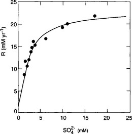
Fig. 5-4 The rate of bacterial sulfate reduction as a function of sulfate concentration. (Adapted from Berner (1984) with the permission of Pergamon Press.)

much less than 5 mM and the sulfate reduction rate does depend on the sulfate concentration (and may be independent of the concentration of organic carbon).

5.4.5 Kinetic Isotope Effects

Molecules containing different isotopic species of an element often react at different rates. The effect is noticeable if the rate-limiting step in a reaction is one in which a bond to the element in question is formed or broken. The primary kinetic isotope effect results from the lower vibrational frequencies of heavier isotopic species. The quantum mechanical zero point vibrational energies are also lower for heavier isotopes and thus slightly more energy is required to break a bond to ¹³C, for instance, than to ¹²C. Isotope ratios may be measured with high accuracy on small amounts of geochemical samples and thus one may infer something about the processes that form a compound from the observed isotope distribution.

For a kinetic isotope effect to exist, the reverse reaction must not occur to a significant extent (in which case we would have a thermodynamic isotope effect) and the molecules undergoing reaction must be drawn from a larger pool of molecules that do not react. If all the molecules are going to undergo reaction there will be no discrimination between isotopes and no kinetic isotopic effect. For these reasons, the kinetic isotope effect for ¹³C in living matter occurs in the early stages of the photosynthetic process when a small fraction of the CO₂ (or) available is added to organic substrates to form carboxylic acids.

Photosynthesis begins with the transfer of CO₂ into the cell from the atmosphere or water. Photosynthetic enzymes then transfer the inorganic carbon to a five-carbon organic compound to form two three-carbon carboxylic acid molecules. (This is the case for the C3 photosynthetic mechanism.) In these steps, reaction of ¹²CO₂ occurs slightly faster than reaction of ¹³CO₂ and the organism has a more negative δ¹³C than the atmosphere or ocean from which it grows. Thus, while marine inorganic carbon has δ¹³C of about 0‰ compared to the reference and atmospheric carbon has δ¹³C of about –7%, the δ¹³C values for plants range from –10 to – 30% (Schidlowski, 1988). The isotope distribution depends somewhat on the species of plant and it is a strong function of whether the plant fixes carbon by the C3 mechanism (most plants) or the C4 mechanism (a smaller group including corn, sugar cane, and some tropical plants).

Isotope effects also play an important role in the distribution of sulfur isotopes. The common state of sulfur in the oceans is sulfate and the most prevalent sulfur isotopes are ³²S (95.0%) and ³⁴S (4.2%). Sulfur is involved in a wide range of biologically driven and abiotic processes that include at least three oxidation states, S(VI), S(0), and S(–II). Although sulfur isotope distributions are complex, it is possible to learn something of the processes that form sulfur compounds and the environment in which the compounds are formed by examining the isotopic ratios in sulfur compounds.

5.5 Non-Equilibrium Natural Systems

Thus far we have studied thermodynamics and kinetics under the assumption that the systems of interest are in equilibrium. However, some natural systems have reaction rates so slow that they exist for long periods under non-equilibrium conditions. The formation of nitric oxide serves as an interesting example.

The net reaction for NO formation is N₂ + O₂ → 2NO, although the actual mechanism by which NO forms does not include the direct reaction of N₂ and O₂ to any significant extent. This direct reaction would involve the breaking of two strong bonds and the formation of two new bonds, an unlikely event. Rather, the oxidation of nitrogen begins with a simple reaction:

1: M + O₂ ↔ O + O + M

This reaction occurs to only a small extent, but the oxygen atoms thus formed may form NO through the following catalytic cycle.

2: O + N₂ ↔ NO + N

3: N + O₂ ↔ NO + O

Net: N₂ + O₂ ↔ 2NO

The reverse reactions of 1, 2, and 3 are also important in establishing the equilibrium between N₂, O₂, and NO₂.

At low temperatures the rates of these reactions are very slow either because the rate constants are very small or because the concentrations of O and N are very small. For these reasons, equilibrium is not maintained at the low temperatures typical of the atmosphere. However, as the temperature rises, the rate constants for the critical steps increase rapidly because they each have large activation energies – E_a = 494 kJ/mol for reaction 1 and 316 kJ/mol for reaction 2. The larger rate constants contribute to a faster rate of NO production, and equilibrium is maintained at higher temperatures. The time scale for equilibrium for the overall reaction N₂ + O₂ → 2NO is less than a second for T > 2000 K.

It may seem unrealistic to consider such high temperatures, but in fact, many processes raise air to very high temperatures. Hydrocarbon or biomass combustion can produce temperatures of 1500–3000 K and lightning discharges can produce temperatures of the order of 30 000 K (Yung and McElroy, 1979). Other processes capable of producing high temperatures include shock waves from comet or meteorite impacts (Prinn and Fegley, 1987) and nuclear bomb explosions (Goldsmith et al., 1973).

As the temperature of an N₂/O₂ mixture is increased above 2000 K the observed concentration of NO (as well as those for NO₂, N, O, and other species) will approach the equilibrium values appropriate for that temperature. As the temperature of the mixture of these gases decreases, the concentrations will follow the equilibrium values. Equilibrium will be maintained as long as the time scale for the chemical reaction is shorter than the time scale for the temperature change (that is, the chemical reaction is more rapid than the temperature change). The time scale for the chemical reaction increases rapidly as the temperature decreases because of the large activation energies. The concentrations of NO at ambient conditions reflect the lowest temperature at which the system was in equilibrium as it cooled.

The example described above for nitric oxide illustrates the interplay between thermodynamics and kinetics. At high temperatures, where the reaction rates are relatively high, the N₂ + O₂ → NO system is in equilibrium. At lower temperatures, however, the rate constants are so low that the system cannot achieve equilibrium and many of the thermodynamic principles described in this chapter would not apply.

The presence of a high concentration of oxygen in the contemporary atmosphere and the prevalence of substances that can react with oxygen in the atmosphere and on the surface of the Earth is another example of a non-equilibrium system.

Photosynthesis produces oxygen by the following redox reaction:

but most of the oxygen thus produced is removed by respiration and decomposition,

A small fraction (less than 1%) of the fixed carbon produced by photosynthesis is buried and physically removed from any potential reaction with oxygen (until the buried material is brought to the surface – at a much later time). Thus, the oxygen in our contemporary atmosphere is the consequence of many millions of years of fixed carbon burial. More details on this topic can be found in Chapters 8 and 11.

The high concentration of oxygen in the atmosphere plays a central role in the photochemistry and chemical reactivity of the atmosphere. Atmospheric oxygen also defines the oxidation reduction potential of surface waters saturated with oxygen. The presence of oxygen defines the speciation of many other aquatic species in surface waters.

Still, a question arises as to why the high concentration of oxygen in the atmosphere does not react with the large amounts of reduced substances present. After all, the reaction between oxygen and fixed carbon is very exergonic; AG for the decomposition reaction above is about – 480 kJ per mole of fixed carbon.

Oxygen concentrations can be high because the rates of many of the reactions of oxygen at ambient temperatures are very slow. The reaction of oxygen and fixed carbon by living systems involves control of the rate by a complex set of enzyme-mediated reactions. In fact, it’s difficult to imagine an extensive range of life on a planet without the presence of reasonable concentrations of reactants that are thermodynamically unstable, but inhibited from undergoing abiotic reaction by high activation energies. Substances that undergo rapid reactions in the absence of enzymes could never reach high concentrations to provide energy for non-photosynthetic organisms. Lovelock (1979) described this connection between extensive life on a planet and the presence of something like oxygen while contemplating ways to recognize the presence of extraterrestrial life on Mars and other planets.

5.6 Summary

Thermodynamics establishes the boundaries of what is possible in the natural world. In many cases enough information is available to enable us to determine the thermodynamic spontaneity of processes. What reaction will occur if a reaction does take place? We often know much less about how fast the reaction is. Will the spontaneous reaction occur within our lifetime? Will the system reach equilibrium? The question of rate involves many issues that are much less well understood. We probably know more about gas phase rates than we do about rates in other media. Even so, it has taken many years to sort out the puzzle of stratospheric ozone depletion. Rates in the aqueous phase and other condensed media are much less well understood. Biological processes involving metabolic pathways in countless organisms, catalytic effects involving trace species, and processes occurring at phase boundaries are among the factors that complicate an understanding of rates in the natural world.

Although many natural systems are far from equilibrium, many localized regions of natural systems are well described in thermodynamic and equilibrium terms. As a general rule, if the reactions that redistribute compounds between the reactant and product states are fast, then equilibrium conditions may be applied. In some cases, part of a system can be described in equilibrium terms and part cannot. As an example, ammonia is generally not in equilibrium with oxidized nitrogen in the atmosphere and surface waters and ammonia is not distributed between the oceans and atmosphere according to equilibrium expressions (Quinn et al., 1988). Nonetheless, the distribution between and NH₃(aq) is described by the usual equilibrium expression because the proton exchange reaction is very fast. Generally speaking, one must be cautious in applying equilibrium relationships unless it is known that the underlying reactions are fast.

Questions

5-1. Consider the reaction N₂(g) + 2O₂ ↔ 2NO₂(g), for which ΔG⁰₂₉₈ = 103.68 kJ/mol and ΔH⁰₂₉₈ = 67.70 kJ/mol. (a) Evaluate K_p for this reaction at 298 K. (b) For the atmosphere at sea level, P_O₂ = 0.21 bar and P_N₂ = 0.79 bar. Evaluate the pressure of NO₂ in equilibrium with these pressures of O₂ and N₂ at 298 K. (c) Evaluate K_p at 500 K assuming that ΔH⁰ is independent of temperature.

5-2. To illustrate an equilibrium involving different phases, consider the following important example. This could represent the equilibrium between a raindrop and atmospheric carbon dioxide:

(a) Show that The equilibrium constant is related to the Henry’s Law constant, M/bar at 25°C. It is often a very good approximation to equate the mole fraction of water to one. (b) If ΔG⁰ for H₂O(l) is –237.18 kJ/mol, and ΔG⁰ for CO₂(g) is –394.37 kJ/mol, estimate ΔG⁰ for H₂CO₃(aq). (c) If ΔH⁰ for the reaction is –20.4 kJ/mol, estimate the Henry’s Law constant at 30°C. (The answer to (c) points to the connection between a negative enthalpy change and a decrease of the equilibrium constant with increasing temperature. See the discussion on the actual states of “CO₂” in water in Section 5.2.4.)

5-3. Evaluate the alkalinities of the following solutions: (a) 0.10 M KHCO₃. (b) 0.10 M K₂CO₃. (c) 0.10 M Ca(OH)₂. (d) 0.10 M NH₄Cl.

5-4. The ratio of ¹⁸O to ¹⁶O atoms is about 2045:1000000 in ocean water. (a) Suppose that 10⁶ atoms of ¹⁶O water evaporate in equilibrium with ocean water at 298 K. How many ¹⁸0 atoms will be associated with these ¹⁶O atoms in the atmosphere? (b) Suppose now that the mixture of isotopes drifts to higher latitudes and is cooled to 293 K, whereupon half of the ¹⁶O atoms condense to form raindrops. What number of ¹⁸O atoms will condense and what number will remain in the atmosphere? (c) Evaluate δ¹⁸O for the precipitation that forms in (b) and for the vapor that remains in the atmosphere. Describe how δ¹⁸O will change as the moist air moves to yet higher latitudes and further condensation occurs.

5-5. Evaluate E⁰ for the reduction of to (3H⁺ + + 2e⁻ → + H₂O). ΔG⁰ values (all in kJ/mol): (–744.6), (–527.8), H₂O (–237.18).

5-6. Write a balanced reaction for the spontaneous process when we allow a path for electron flow between the O₂/H₂O electrode and the H⁺/H₂O electrode as described in Section 5.3.3.

5-7. In thinking about sulfur in the environment, we may need to include the pg lines for the O₂/H₂O/H₂ system. The line describing pε for O₂ at 1.0 bar in equilibrium with H₂O will lie above all of the sulfur diagram for the pH range 0 to 14. (a) If pε for electrons in equilibrium with O₂/H₂O is more positive than pε for electrons in equilibrium with/S⁰, which electrons will have greater activity? Will a spontaneous reaction occur involving O₂/H₂O and/S⁰?(b) Would you expect a sulfate solution to be stable in water saturated with O₂? (c) Would you expect a solution that is 0.10 M in HS⁻ andw in contact with 1.0 bar O₂ to be stable? What spontaneous reaction (if any) might occur?

5-8. Consider the NO/NO₂-catalyzed ozone destruction cycle, reactions 5 and 6 in Section 5.4.3. One could perform a calculation to determine which reaction is the rate-limiting step (i.e., the slowest step that determines the rate of the overall reaction) in this cycle. In this case, a theoretical doubling of k₅ reduces the ozone concentration by about 2%. On the other hand, doubling k₆ reduces the ozone concentration by nearly 50%. (a) Which reaction is the rate-limiting step in NO/NO₂-catalyzed ozone destruction? (b) The concentrations of NO and NO₂ are: [NO] = 2.9 × 10⁸/cm³ and [NO₂] = 6.1 × 10⁹/cm³. How do these data support or refute your answer to (a)?