Ice Sheets and the Ice-Core Record of Climate Change
18.1 Introduction
18.1.1 Historical Context
In the mid-19th century, Louis Agassiz and colleagues recognized that many features of the landscapes of northern Europe and North America could be sensibly explained only as products of glaciation (Agassiz, 1840). These features include bouldery ridges (called moraines) crossing flat lands, enormous boulders found far from their sources, deep lake basins, and ancient channels of enormous rivers. The realization that much of the now densely populated regions of Europe and North America were rather recently buried by ice lead to a startling revelation: the Earth experiences environmental changes of spectacular magnitude and global significance. Subsequently, careful analyses of the glacial deposits revealed that there had been at least several major episodes of glaciation. In the 1950s and 60s new geochemical and paleontologic tools painted a much more complete picture of these ice ages. In particular, the oxygen isotopic composition of seawater, whose history can be learned by analyzing cores of ocean-floor deposits, is a measure of continental ice-sheet volume. These data revealed that there were 30 or so major periods of glaciation over the past two million years, and these occurred with considerable temporal regularity.
Such major environmental changes present a tremendous opportunity for studying Earth systems and biogeochemical cycling. These changes may be viewed as global-scale experiments that have already been conducted for us. By elucidating their nature (the histories of both forcings and environments), we can learn much about the behavior of coupled Earth systems.
Records of past environmental change are preserved in a broad range of Earth materials. Past environments are inferred from “proxy” records, meaning measurements of physical and chemical parameters of marine and terrestrial sediment, polar ice, and other materials that were in some way influenced by their environment during accumulation. Examples of proxy records are the distribution of glacial deposits, the isotopic composition of terrestrial and marine sediments and ice, the abundance and species composition of plant and animal fossils, and the width of tree rings.
18.1.2 This Chapter
This chapter is a brief introduction to Earth’s historical environmental changes, with emphasis on the recent ice-age cycles. We chose this emphasis because preservation of these environmental records is much better than for earlier times, and because the ice ages constitute drastic changes in global environment which have occurred throughout the past two million years (the Quaternary) despite the constancy of the major boundary conditions controlling climate (solar luminosity, positions of the continents). Understanding the causes of these changes is crucial for assessing the modern environment’s potential for change. Current understanding is far from complete.
We will further focus much of this chapter on paleoclimate records obtained by analyzing ice cores extracted from the polar ice sheets. There are many important types of paleoclimate records, but the ice-sheet records have special importance. The ice sheets are the only significant accumulations of atmospheric sediment and therefore contain unique information about atmospheric composition and processes. In particular, atmospheric gases are trapped in glacial ice, so ice-core analysis can rather directly reveal changes in greenhouse gas composition through time. Readers wishing to see a more comprehensive treatment of the material in this chapter are referred to Crowley and North (1991) for general paleoclimatology, and Hammer et al. (1997) for ice-core studies.
The goal of this chapter is twofold: first, to present some of the most important aspects of Earth’s environmental history, and second, to communicate the power, complexity, and incompleteness of paleoclimatology through a presentation of one of its most important tools.
18.2 Quaternary Climate Change
18.2.1 Context
Over the last 60 to 70 million years the Earth has gradually cooled by 5 to 15°C and sea level has fallen by more than 200 m. Possible causes of this trend include changes in land distribution, ocean circulation, and atmospheric CO2. The land area in northern high latitudes has increased, and this may have allowed the growth of large ice sheets, resulting in cooler climate due to the increase in Earth’s albedo ( Chapter 7) (Turekian, 1996). Models and proxy measurements (Cerling et al., 1993; Berner, 1990) suggest that atmospheric CO2 content decreased substantially during this time, from values of 1000–2000 ppmv in the Cretaceous to 200–280 ppmv by the late Quaternary. One proposed explanation for this CO2 drawdown is continental weathering accompanying the uplift of high mountain ranges (Raymo and Ruddiman, 1992). Mountain uplift could also cool and dry the global climate by directly affecting large-scale atmospheric circulation and precipitation patterns (Ruddiman and Kutzbach, 1991). There is considerable debate, however, about whether increased mountain uplift was a cause or consequence of the climatic cooling of the past five million years which finally plunged Earth into the ice ages (Molnar and England, 1990). Nonetheless, in all these scenarios, the root cause of Earth’s cooling from the balmy Cretaceous to the modern glacial ages is the slow tectonic motions of the Earth’s lithospheric plates (see Chapter 9).
18.2.2 The Tempo of Quaternary Climate Change: Oxygen Isotopes and Orbital Forcing
In addition to being relatively cool, the climate of the last two million years has been quite variable. The early studies of glacial deposits on land established that Earth’s climate was much colder than present in the very recent geologic past, only a little over 10 millennia ago. Further studies indicated that periods of glaciation were interrupted by warm climates. More recently, a detailed picture of Quaternary climate changes has emerged from studies of ocean sediments. The largest amount of paleoclimate information from these sediments has come from studies of variations in abundance and species composition of planktonic (surface-water dwelling) and benthic (sea-floor dwelling) microscopic plants and animals, and the oxygen and carbon isotopic composition of the calcium carbonate shells of these organisms.
In modern sediments particular assemblages of species are characteristic of particular environmental conditions. Therefore it is possible to use species assemblages in ancient sediments to infer past sea-surface temperatures and other variables, and these techniques provide a wealth of paleoclimate information. Complementary information is provided by the oxygen isotopic composition of marine plankton’s calcium carbonate shells, which has varied significantly throughout the Quaternary. The δ18O(see Box 1) of these shells is a function of both the δ18O and the temperature of the water in which the shells grow. The measurements of δ18O on sea-core sediments therefore reveal a combined history of ocean temperature and ocean δ18O. Emiliani (1955) initially interpreted the Quaternary marine δ18O record as primarily an indicator of temperature change. Subsequent work (Shackleton, 1967) revealed that much of the signal instead resulted from changes in sea water δ18O, due to changes in volume of continental ice sheets and glaciers (see Section 18.3.2.1 below). The marine δ18O record is now interpreted primarily as a record of changes in continental ice volume. Continental ice volume expands (and ocean δ18O increases) during cooling climates as northern hemisphere ice sheets form and grow and the Antarctic ice sheet expands. Thus marine δ18O is a proxy for global climatic temperature, with high marine δ18O indicating cold climates. Because large-scale climate changes are required to grow large continental ice sheets, marine δ18O is one of the single best proxies for global climatic changes.
The two most common isotopes of oxygen are 16O and 18O, and the two natural isotopes of hydrogen are 1H and 2H or D (deuterium). If a sample of carbonate contains C18 moles of 18O and C16 moles of 16O, then define the heavy:light ratio as R18 = C18/C16. Similarly, natural water molecules are mostly of three types: H216O, H218O, and HD16O. For a given sample of water, call the number of moles of each W, W18, and WD, respectively. Then define the heavy:light ratios as R18 = W18/W and RD = WD/W. For either water or carbonate, theδ are defined as deviations of these ratios from standard values for these ratios (call the ratios of the standards S18 and SD):

For water, the standard ratios are approximately the average ratios for modern seawater (these standards are called SMOW, or Standard Mean Ocean Water), so δ18O and δD both equal zero for modern seawater (if a standard other than SMOW is used, this will not be true). δ values are typically very small numbers and so are usually multiplied by 1000, in which case the units are “per mil.”
Numerous studies of marine δ18O histories (and the strongly correlated species assemblages) demonstrate that global climate variations have followed a characteristic quasi-cyclic pattern over the past 2 Myr(Fig. 18-1). Dominant in the last 700 kyr of these records is an approximately 100 kyr cycle of glacial and interglacial periods (prior to this time an ∼40 kyr cycle dominated). This 100 kyr cycle has a characteristic asymmetrical “sawtooth” shape, with gradual descents into cold climate followed by abrupt terminations of glacial conditions and return to warm interglacial climate (Broecker and Denton, 1989). The warm interglacial climates are generally of brief duration relative to the whole cycle.
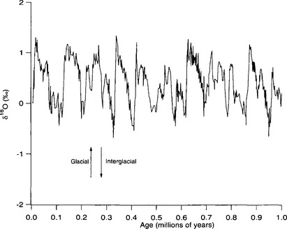
Fig. 18-1 Benthic foraminiferal oxygen isotope record from 3477 m water depth in the eastern tropical Pacific ocean from Ocean Drilling Program site 677 (Shackleton et al., 1990). 18O/16O ratios are expressed in the δ notation relative to the SMOW standard. Note the strong 100 kyr periodicity characteristic of Quaternary climate records.
Much of the variation in these time series for the past 700 kyr can be described by a combination of a 100 kyr cycle plus additional cycles with periods of ∼20 and ∼ 40 kyr. This result immediately suggests that the ice-age cycles are caused by variations in the amount and seasonally of solar radiation reaching the Earth (insolation), because the ∼20, ∼40, and ∼ 100 kyr periods of climate history match the periods of cyclic variations in Earth’s orbit and axial tilt. The hypothesis that these factors control climate was proposed by Milutin Milankovitch in the early part of the 20th century and is widely known as “Milankovitch Theory.” It is now generally accepted that the Milankovitch variations are the root cause of the important 20 and 40 kyr climate cycles. The 100 kyr cycle, however, proves to be a puzzle. The magnitude of the insolation variation at this periodicity is relatively trivial, but the 100 kyr cycle dominates the climate history of the last 700 kyr. Further, the insolation forcings do not directly predict the asymmetrical “sawtooth” form of the main cycles.
The three orbital parameters that control the amount and seasonality of incoming radiation are the tilt of the Earth’s spin axis, the eccentricity of the Earth’s orbit, and the precession of the equinoxes(Fig. 18-2). The tilt of the spin axis varies between 22° and 25°, with a period of 41 kyr. The eccentricity of the Earth’s elliptical orbit varies from nearly circular to 6%, with periods of 100 and 400 kyr. Precession of the equinoxes refers to the continual change in the timing of the seasons relative to the position of the Earth along its eccentric orbit (which determines the Earth to sun distance). Two processes influence equinox precession. First, the Earth’s spin axis does not have a fixed orientation in space, but rather wobbles in such a way that the geographic north pole describes a full circle in space every 26 000 years (Polaris is not always the North Star). Second, the ellipse of the orbit itself also rotates slowly, with a period of 22 000 years. The interaction of these two generates precession cycles with periods of 19 000 and 23 000 years.
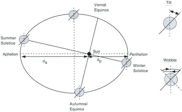
Fig. 18-2 Orbital parameters that control the seasonal and annual receipt of radiation at the Earth’s surface. The Earth’s rotational axis tilts and wobbles as shown. The eccentricity of the orbit is (dp – da)/(dp + da) which is zero for a circle but for the Earth’s orbit is sometimes as large as 0.06. (After Hartmann (1994, p. 303) and Turekian (1996, p. 80).)
What is the effect of these orbital variations on the input of solar radiation to the Earth? The precession cycles cause changes in the seasonal distribution of insolation. The seasons exist because the Earth’s spin axis is tilted. Northern hemisphere summer occurs when the Earth’s spin axis points toward the sun, and on the summer solstice the sun lies in the vertical plane containing the spin axis. Currently the summer solstice occurs at a position along the elliptical orbit for which the Earth-sun distance is near its maximum value (aphelion). Through time, the precession cycle shifts the position of the solstice along the orbit so that the Earth-sun distance on the day of summer solstice varies through time. Northern hemisphere summers are colder, and southern hemisphere summers warmer, if the summer solstice occurs when the Earth-sun distance is a maximum, as it is in the modern day. Eleven thousand years ago, when ice sheets were melting, the situation was reversed; northern hemisphere summer occurred while the Earth was closest to the sun (near perihelion), and summertime northern hemisphere insolation was greater than that today. Thus precession creates cyclical variations in seasonal radiation at periods of 19 and 23 kyr, and these variations are opposite in the northern and southern hemispheres. Compared to other Milankovitch forcings, precession causes the largest seasonal variations at low latitudes. The net global radiation received over a year is not affected by precession.
Tilt variations also do not affect the annual total of solar energy received by the whole Earth, but do change the annual total for polar regions (simultaneously for both hemispheres). Tilt also affects the seasonal insolation at high latitudes, with greater tilt leading to warmer summers and cooler winters in both hemispheres.
Eccentricity variations change the average Earth-sun distance such that annual insolation changes by approximately 0.2%, or 0.5 W/m2 at the Earth’s surface (Crowley and North, 1991). This is small compared to the 10% seasonal changes associated with the other Milankovitch cycles. That a 100 kyr periodicity characterizes both the eccentricity and the glacial-interglacial cycles may reflect an important role for the eccentricity cycle in causing exceptional highs of seasonal insolation (in concert with the other Milankovitch forcings) which may be necessary to terminate glaciations. How, and if, the eccentricity cycle influenced Quaternary climate is a major question in current research. An alternative, and not yet fully tested, explanation for the 100 kyr cycle is that there actually is a significant astronomical forcing of this period, related to tilt of the ecliptic with respect to a horizon of interstellar dust (Muller and MacDonald, 1997). Despite this uncertainty concerning the 100 kyr cycle, the marine oxygen isotope record provides convincing evidence that changes in the Earth’s orbit and tilt are a root cause of some climate changes throughout the Quaternary (Hays et al., 1976). Considerable effort has been devoted to understanding this connection. The match between periodicities of insolation and climate is robust, but many analyses have shown that the timing of insolation changes and global climate changes are correlated only if insolation is taken to be that for summer at mid-high latitudes in the northern hemisphere. This suggests the fundamental link between Milankovitch forcings and climate involves increased glacier melt rates during very warm summers, without opposing changes in very cold winters. In this way, greater seasonal contrast leads to the growth and decay of the great ice sheets on North America and Eurasia.
Though an important part of the Quaternary climate puzzle, this view of the ice-age cycles is by itself quite incomplete. If Milankovitch forcings alone govern climate change then:
1. Most climate variability will occur with 20 and 40 kyr periods.
We have already shown that 1 is not generally true. Later in this chapter we show that 2 and 3 are not generally true either. Thus there are additional important elements of the climate change engine.
18.2.3 A Closer Look at Glacial to Interglacial Climate Change
There is a much better record of the last major transition from glacial to interglacial climate than for earlier portions of the climate cycles. This transition therefore provides a useful starting point for examining the character of major climate changes, though each of these may have had unique elements.
18.2.3.1 The Ice-Age Earth
Approximately 20 kyr ago glaciation had attained its maximum extent (a time called the last glacial maximum or LGM). Much of Canada and the northern United States, as well as northern Europe and Asia, were covered by large ice sheets that in places exceeded 3 km in thickness(Fig. 18-3). Although the growth of these major ice sheets was the most dramatic change of the Earth’s surface, smaller ice caps and glaciers also advanced during the last glacial maximum. In Antarctica the West Antarctic ice sheet expanded significantly during the LGM (Denton et al., 1989), while the East Antarctic ice sheet expanded modestly. Concurrent with the growth of major ice sheets was a drop in sea level, with a maximum sea level depression during the LGM of approximately 120 m (Shackleton, 1987).
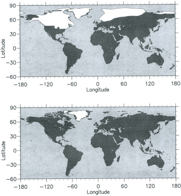
Fig. 18-3 Extent of ice sheet cover (shown as white) during the LGM (top panel) compared to modern (bottom panel), excluding Antarctica. Locations of ice sheets are approximate.
The Earth was drier than present during the LGM, and the hydrologic cycle slower. Polar snow accumulation rates were significantly depressed. Delivery of continental dust to the ice sheets and the ocean was enhanced, suggesting overall higher levels of aridity. Many studies of fossil pollen, and geomorphic features like sand dunes, support this view. Some regional exceptions existed; wet areas during the LGM included the Great Basin of North America, and portions of Russia, the Middle East, southern South America, and southern Australia (COHMAP, 1988; Crowley and North, 1991). Studies of terrestrial fossils, and pollen in particular, reveal equatorward shifts of vegetation zones during colder climates, and suggest that local climate changes were highly variable. Viewed as a whole, the terrestrial and marine records consistently show that environmental changes in polar regions were much greater than those in equatorial regions.
18.2.3.2 Global Temperature Change
In the 1970s the CLIMAP project compiled the analyses of marine sediment fossil assemblages (CLIMAP members, 1976) to produce global maps of sea surface temperatures during the LGM. These suggested that sea surface temperatures in the mid to high latitudes were depressed by up to 6 to 10°C, that areas of seasonal sea ice were larger, and that polar fronts were shifted to lower latitudes. Pollen-based reconstructions of mid-high-latitude land temperatures suggest temperature depressions of 4 to 8°C in the mid latitudes, and larger changes adjacent to the ice sheets. CLIMAP reconstructions for many areas of the tropics indicate little or no change in sea surface temperature, in contrast to the mid-high-latitude data. This appears inconsistent with locations of glacial deposits in New Guinea, Africa, South America, and Hawaii, all of which show that snowlines were depressed during the glacial period by up to 1000 m below modern levels. The latter suggests a much larger tropical temperature depression, approximately 5–6° C based on the 6° C/km decrease of temperature with increasing altitude in the troposphere. This conclusion is supported by newer paleotemperature proxies, including the noble gas composition of glacial age groundwater in tropical aquifers (Stute et al., 1992, 1995), and the Sr/Ca ratio of coral skeletons (Guilderson et al., 1994). However, it is possible that tropical temperature depression varied regionally. The magnitude and patterns of glacial-interglacial temperature change in the tropics remain subjects of active research.
18.2.3.3 Ocean Circulation
In the modern world, oceanic heat transport has a prominent role in determining global and regional climates. Colder ocean waters during the LGM suggest reduced LGM oceanic heat transport on average, but such changes cannot be inferred without knowledge of circulation changes too. Several geochemical proxies record ocean circulation changes. Most important are the carbon isotopic composition (δ13C) and the Cd/Ca ratio of planktonic and benthic foraminifera (Curry et al., 1988; Boyle et al., 1988). Cycling of both parameters depends on biological productivity in surface waters. Surface-water dwelling organisms preferentially remove 12C and Cd from surface waters and the rain of their carcasses to the deep sea causes surface waters to be depleted in Cd and enriched in 13C.
After transport to the deep sea (see Chapter 10), these surface-derived waters gradually enrich in Cd and 12C. More vigorous transport (meaning more vigorous formation of deep water and vertical mixing of the global ocean) causes deep waters to have lower Cd/Ca and higher δ13C, and this signal is recorded by benthic foraminifera. Much attention has focused on the deep-water formation sites in the North Atlantic Ocean, because these are coupled to the tremendous northward transport of heat by the Gulf Stream. Studies of foraminifera Cd/Ca and δ13C show that the formation of North Atlantic Deep Water was greatly reduced during the LGM, and replaced by formation of shallower intermediate water. This probably means that Gulf Stream heat transport was greatly reduced. Longer time-series indicate that variability in deep-water production was a general characteristic of glacial-interglacial cycles (Raymo et al., 1989). Further, rapid variations in deep-water formation correlate with rapid climate changes during the last glacial period (see 18.3.2.4). Thus changes in ocean heat transport likely have a large role in the climate cycles (Broecker and Denton, 1989).
18.3 Ice Sheets as Paleoclimate Archives
We now explore in detail the methods and results of ice-core paleoclimatology. The reward for this effort is an astonishing expansion of our knowledge of past environments, remarkable both for its implications and its level of detail.
18.3.1 Ice-Core Basics
In the interiors of ice sheets, there are boundaries (usually coincident with topographic ridges on the ice-sheet surface) separating regions where ice flows in one direction from regions where ice flows in the opposite direction. These boundaries are analogous to drainage divides separating watersheds, and are therefore called ice divides. At the ice divide, the ice motion is predominately vertical downward(Fig. 18-4) and sluggish so that ice deposited as snow on the surface at this one location accumulates there for a long time. Due to the spreading of the ice flow lines, a block of ice deposited at the surface is horizontally stretched as it descends, which causes the block to thin vertically, because volume of the block is conserved. Thus, the age of ice increases exponentially with depth beneath the ice divide. By extracting a core of ice at, or near, an ice divide, one can obtain a continuous record of atmospheric sediment that contains more and more years per length of core near the bottom. Core extraction is usually done with a drill that mechanically cuts a cylinder of ice, typically 10 to 15 cm in diameter. The locations of many important core sites are shown inFig. 18-5.
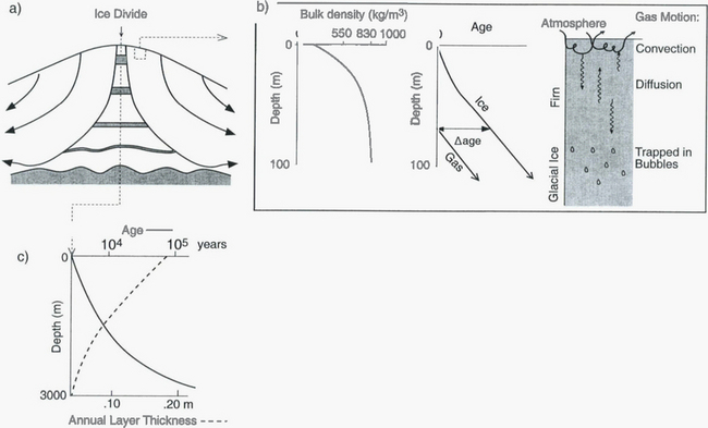
Fig. 18-4 (a) Cross-section through an ice divide showing flow lines and thinning of layers. (b) Closer look at the upper 100 m: characteristic density variations, age-depth relations for ice and gas, and mechanisms of gas transport. (c) Characteristic depth-age relation and annual layer thicknesses, with numbers chosen to represent central Greenland. Age axis is non-linear.
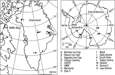
Fig. 18-5 Locations of important ice-core sites in Greenland and Antarctica The two central Greenland sites, GISP2 and GRIP, are collectively known as Summit. (after Paterson, 1994).
For an ice sheet of thickness H in equilibrium with a climate supplying accumulation at a rate (thickness of ice per unit time), the vertical velocity near the ice-sheet surface is
 and this velocity decreases to zero at the ice-sheet bed. A characteristic time constant for the ice core is
 The longest histories are therefore obtained from the thick and dry interiors of the ice sheets (particularly central East Antarctica, where
 ). Unfortunately, records from low
 sites are also low resolution, so to obtain a high-resolution record a high
 site must be used and duration sacrificed (examples are the Antarctic Peninsula
 and southern Greenland
 ).
).
18.3.1.1 Depth-age scales
Obtaining an accurate and detailed depth-age relationship for an ice core is, of course, a necessary task for learning paleoclimate histories. Approximate time scales can be calculated using numerical models of ice and heat flow for the core site (Reeh, 1989), constrained by estimates of the modern accumulation rate and by measurements of ice thickness from radio-echo-sounding surveys.
Once a core is extracted, measurements of seasonally varying properties allow identification of annual layers (Hammer et al., 1987). Counting these along the core, as one would count rings in a tree, yields a depth-age scale of high precision and very good accuracy. Useful seasonally varying properties include dust content, isotopic composition, concentrations of some chemical impurities, electrical conductivity (a proxy for core acidity), and physical stratigraphy (seen as variations in transmitted light seen through a sliced core). Annual layers must be preserved in the ice sheet for absolute age determination to be possible in this fashion. Annual layer preservation is good at high accumulation-rate sites in Greenland and West Antarctica, but not at the very dry sites in East Antarctica. In addition to such continual counting methods, one can determine the absolute age of ice by identifying the fallout from volcanic eruptions of known age.
The rapid global mixing of gases in the Earth’s atmosphere, in a few years’ time, enables powerful techniques for learning the depth-age scale of an ice core by correlating the variation of gases along one core to the same variations along another core for which absolute ages are known, and to marine sediment cores. Of particular use are the δ18O of O2 gas (Sowers et al., 1993; Bender et al., 1994) and methane (Blunier et al., 1998; Steig et al., 1998).
A very important complication in interpreting ice core records, and in defining depth-age relations, is the fact that snow transforms to ice 50 to 100 m below the surfaces of most polar ice sheets. This means the gas trapped in ice is actually younger than the solid ice at the same depth, and that a variety of processes can transport and redistribute gases in this snowy upper layer (called the firn). To understand this, and to prepare for subsequent discussions, we must discuss how snow converts to ice near the ice sheet surface.
18.3.1.2 Firn and gas trapping
At the ice-sheet surface, motion of water vapor very rapidly converts faceted and angular snow to solid ice spherules. Subsequently, the weight of overlying accumulation forces these into a more compact configuration by slip at their boundaries and creep deformation. Thereby the density of a given layer steadily increases through time, from a value of approximately 300 kg/m3 at deposition to an ultimate value of approximately 920 kg/m3 for glacial ice. Thus there is a marked increase of density with depth below the surface, with most of the variation occurring in the upper 100 m. Correspondingly, the air-filled pore spaces between ice grains become smaller and more isolated as depth (or age) increases. These pores are finally isolated as distinct bubbles at a bulk density of around 830 kg/m3. Above this level, which is generally 40 to 100 m deep, air spaces are interconnected and open to the atmosphere above. This entire zone is called the firn. In the firn, gases are free to move to and from the atmosphere, by wind-driven convection in the upper 10 m and by diffusion below this(Fig. 18-4). Thus the gas trapped in bubbles is younger than the age of the adjacent ice. This gas-age-ice-age difference (often referred to as Δage) today ranges from 30 years at ice-core sites with very high accumulation rates (> 100 cm/yr) to greater than 2000 years at low-accumulation-rate sites (<2 cm/yr). During glacial times, when snow accumulation rates were lower, Δage was larger. Below the firn is “glacial ice,” which retains visible bubbles until depths of 1500 m or so, where the gases finally are incorporated into the solid lattice as clathrates.
The interstitial air trapped during this process preserves a largely unaltered record of the composition of past atmospheres on time scales as short as decades and as long as several hundred thousand years. Such records have provided critical information about past variations in carbon dioxide (CO2), methane (CH4), nitrous oxide (N2O), carbon monoxide (CO), and the isotopic composition of some of these trace species. In addition, studies of the major elements of air: nitrogen, oxygen, and argon, and their isotopic composition, have contributed greatly to understanding of past climates and the processes that trap gases in ice. Gas records are discussed in Sections 18.3.2.3 and 18.3.5.
18.3.2 Thermometry: Tools and Results
18.3.2.1 Stable isotopes in water
One of the most important measurements made on an ice core is the isotopic composition of the water molecules composing the ice (Dansgaard, 1964), specifically δ18O and δD(see Box 1). Several complementary techniques that also reveal temperature histories are described further inSections 18.3.2.2 and 18.3.2.3. Consider a schematic cross-section through the Earth from low latitudes to the poles(Fig. 18-6). Water evaporates from the oceans in the subtropics (some moisture, not shown here, is contributed by the continents and the polar oceans as well) and is transported generally poleward. Along this path, the air mass cools as it rises and radiates heat, and consequently water vapor condenses and precipitates, progressively depleting the air mass of water along this path. Eventually this air mass snows onto the ice sheet. At each stage of this process, when water vapor is converted to liquid or solid, the heavy isotope of oxygen is preferentially removed from the vapor. Thus the vapor becomes progressively lighter and lighter isotopically along this path (see Box 2), so that the snow accumulating on the ice sheet is substantially isotopically lighter than the original source. In fact, ice sheets are so much isotopically lighter than the ocean that the growth and disappearance of ice sheets through the glacial-interglacial cycles causes significant changes to the δ of the ocean, despite its tremendous volume. The ocean becomes heavier by 1.2%o during extremes of glacial climate. This is the primary explanation for the δ18O variations of deep-sea sediments(discussed in Section 18.2.2).
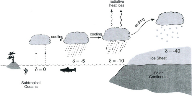
Fig. 18-6 Characteristic air-mass trajectory and corresponding per mil isotopic composition of precipitation, along a transect from the subtropics to a polar ice sheet. This is a highly schematic view of the true atmospheric system.
Further considering the system displayed inFig. 18-6 the total isotopic “lightening” of the vapor is a direct function of the fraction of water mass removed from the air. This fraction in turn is a function of the net cooling of the air mass. This suggests that S measured at the ice core site should be useful as some sort of thermometer. Most directly, it is a measure of the total temperature drop from source to the precipitating clouds over the ice-core site (see Box 2). Indeed, if one visits many locations on an ice sheet and measures the mean annual δ and the mean annual temperature at these sites, a very strong correlation between δ and temperature is found(Fig. 18-7). This is true both for the Greenland ice sheet and the Antarctic ice sheet, and for high-latitude precipitation in general (Jouzel et al., 1987). The strength of these correlations suggests that measurements of δ along an ice core may give an accurate, quantitative view of temperature history at the core site.
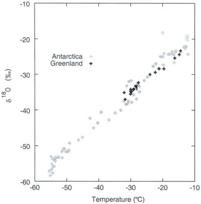
Fig. 18-7 Observed correlation of isotopic composition with temperature for near-surface snow in Greenland (Johnsen et al., 1989), and Antarctica (Dahe et al., 1994).
Box 2: Stable Isotope Tutorial
The global atmospheric circulation acts as an enormous filtration system, which depletes high-latitude precipitation of heavy isotope-bearing water molecules. Because of this system, measurements of the stable isotopic composition of the ice sheets and of ocean-floor sediments reveal very important paleo-environmental information (see Sections 18.2.2,18.3.2, and 18.3.3). Here we examine this filtration system at a physical level. This system was first understood by a great Danish geochemist named Willi Dansgaard (Dansgaard, 1964).
Tutorial: Equilibrium Processes
Inside the air mass moving poleward inFig. 18-6 there are moles of
 vapor,
 moles of
 vapor, and
 moles of HDO vapor. Write
 to signify either of the heavy-isotope-bearing vapors
 . Define the isotopic ratio of the vapor as
 . If the condensation of the vapor to form liquid water or solid ice is an equilibrium process, and this condensation is quickly removed from the air mass as precipitation, the corresponding isotopic ratio in the precipitation (Rpj) is proportional to that of the vapor

where the fractionation factor a is slightly greater than one, and is different for the deuterium and 18O systems. Call these α18 and αD respectively. At Earth surface temperatures, values for these range from 1.008 to 1.025 for α18 and 1.07 to 1.25 for αD and these are temperature dependent, and different for liquid-vapor and ice-vapor equilibrium (Horita and Wesolowski, 1994; Majoube, 1971; Merlivat and Nief, 1967). The definition of δ for the precipitation is (see Box 1)
where either Rs is a standard ratio. Note that the δ values for vapor and condensate (δv and δp) in equilibrium are related by
Differentiating both (B1) and (B2) shows that changes in the composition of precipitation and the composition of the vapor are related by
From the definition of Rv:
Mass conservation and equilibrium fractionation together require that
Combining (B4), (B5), and (B6) shows that
As water is almost entirely we can replace
 in (B7) with Nv where Nv is the total moles of water vapor in the air mass:
which describes a Rayleigh distillation process (Merlivat and Jouzel, 1979). The quantity Nv in a specified amount of air is proportional to the ratio of vapor pressure to total pressure, in accordance with the gas law. When precipitating, the air is nearly saturated with water vapor, so Nv per mass of air is directly proportional to the saturation vapor pressure es and inversely proportional to the total pressure P

The saturation vapor pressure is strictly a function of temperature as indicated by the Clausius–Clapeyron equation

where the constant Δ = 5435K. It is this basic thermodynamic principle that makes δ a thermometer. We can now integrate Equation (B8) to see how the isotopic composition of precipitation δpj changes as an air mass cools and its mixing ratio decreases (recall the j refers either to the 18O system or the deuterium system). It is instructive to first consider an approximation wherein αj has a constant (average) value . In this case Equation (B8) is easily integrated between initial and subsequent δpj values (δ0pj and δpj) and vapour contents (Nv0 and Nv) to show
into which we substitute (B9) and (B10) to show that, in terms of initial and subsequent temperatures (To and T) and pressures (P0 and P)
The thermometric nature of δ is clearly seen, and in particular the dependence of δ on the temperature drop from initial condensation temperature to final condensation temperature. In addition, δ depends on its initial value (the source-region composition δ0j) and on the net pressure change. This pressure dependence is not important for temporal changes in δ at ice core sites in the interiors of Antarctica and Greenland, but is important for the spatial variation in δ across the ice sheets. It may also be important at sites closer to the ice sheet margins, where elevation may have changed considerably through glacial—interglacial cycles. An example of the predicted isotope-temperature distribution with constant a using (B12) is shown inFig. 18-23. Now let us abandon our heuristic assumption of constant a. In reality, the fractionation is significantly enhanced at low temperatures; between 20°C and – 40°C (α18 – 1) increases by a factor of 1.3 and (αD– 1) increases by a factor of 1.6. This includes a 30% and 10% increase, respectively, at the transition from liquid-vapor equilibrium to ice-vapor equilibrium. This temperature dependence is not the primary reason for the thermometric properties of δ but it does enhance the sensitivity of δ to T in the polar regions, and must be included in calculations. An example of integrating Equation (B11) to solve for δ with the proper temperature dependence is shown inFig. 18-23. Achieving a good δ(T) prediction at low temperatures requires incorporating non-equilibrium fractionations (Jourel and Merlivat, 1984).
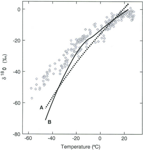
Fig. 18-23 Observed correlation of isotopic composition of precipitation with ground temperature (gray diamonds; Jouzel et al., 1987), and predictions of simple isotopic models. A, prediction with constant a; B, prediction with temperature-dependent α.
Meteoric Water Line and Deuterium Excess
Now consider the simultaneous evolution of δ18O and δD. Suppose an air mass having initial compositions δj = 0 cools and precipitates, always as an equilibrium process. According to the preceding analysis, measurements of both isotopic ratios in precipitation will plot on a curve with a slope approximately given by
which is very nearly a constant with a value between 7 and 9. This is the primary explanation for the Meteoric Water Line (see Section 18.3.3), which has a slope of 8 (Fig. 18-24). Deviations from a line of slope eight and zero intercept are called deuterium excess, .
.
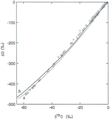
Fig. 18-24 Observed correlation (the Meteoric Water Line) of the two most important isotopic ratios in precipitation (gray diamonds; Jouzel et al., 1987 and Dahe et al., 1994), and predictions of simple isotopic models. A, prediction with constant α; B, prediction with temperature-dependent α.
Equilibrium isotopic fractionations explain the gross behavior of δ18O and δD in precipitation of mid to high latitudes.
The utility of δ as a thermometer gains further support from direct measurements showing correlation of temperature and δ of precipitation through time over seasonal cycles (Shuman et al., 1995). At longer temporal scales, temperature measurements in boreholes and gas composition measurements both provide temperature information which can be compared to δ. Results from such comparisons have so far supported the use of δ as a qualitative thermometer, but not a quantitative one.
There are many reasons to suspect that δ may not be a faithful quantitative thermometer. First, δ of the initial source water(s) can change through time, as ocean composition changes due both to ice-sheet growth and to changes in water flux from the continents. Source-water δ also can change through time as the source-water location (or, more generally, the spatial distribution of sources) changes, as a result of atmospheric circulation changes. Second, as described above, δ is primarily sensitive to the temperature difference between source and site. Therefore, coincident variation of temperature at source and site can significantly dampen δ changes at the ice-core site. δ will work best as a thermometer for the core site if the source temperature changes not at all. Independent variations in source and site temperature could possibly result in a complicated δ record whose meaning is ambiguous.
Important complications occur at the ice-core site. The seasonal variation of δ is much larger than the δ change accompanying climate changes, even for the great glacial-interglacial transitions. Yet precipitation does not necessarily fall uniformly throughout the year. Relatively small changes in the seasonal timing of precipitation could therefore cause changes in δ that may be misinterpreted as significant changes in climatic temperature. Precipitation biasing can be a problem at shorter temporal scales too, in that precipitation over the ice sheets accompanies advection of relatively warm air masses, so there will generally be a warm-weather bias to the stable isotope records.
All these potential complications mean that independent temperature-history information is very useful, though no other temperature reconstruction techniques yet match the very high resolution of these isotopes.
18.3.2.2 Borehole temperatures
The modern distribution of temperature at depth in an ice sheet also contains important paleoclimate information, and in particular provides a relatively direct measure of past climatic temperature at the ice-sheet surface. Near an ice divide, heat is transported downward in the ice via conduction and advection. Given a steady surface temperature (constant climate), the temperature at depth will evolve to have a relatively isothermal upper layer, due to downward transport of ice, and warmer ice at depth, due to heat flux from the Earth and to heat generation in the rapidly deforming basal layers(Fig. 18-8). If the climate warms abruptly, and maintains the new warmer temperature, the heat transfer processes will send a wave of warmth downward into the ice. Subsequent measurements of the temperature–depth distribution will reveal a cold spot, which is a direct remnant of the previous, cooler climate. By mathematically reversing this natural heat flow, we can reconstruct a history of climatic temperature variations through time. This mathematical reversal is accomplished by heat- and ice-flow modeling coupled to geophysical inverse techniques (Dahl-Jensen and Johnsen, 1986; Cuffey and Clow, 1997).
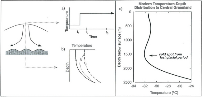
Fig. 18-8 Characteristic temperature–depth distributions at an ice divide. For a climatic temperature history as shown in (a) the temperature-depth distribution changes as shown in (b). Following the step increase in surface temperature, the initial steady temperature profile (t1 in (b)) is altered by a warming wave (e.g., at time t2) but eventually reaches a new steady profile by time t3. (c) Temperature data from Greenland measured by Gary Clow of the US Geological Survey, showing wiggles due to climate variations (Cuffey et al., 1995).
There are severe limits on the recoverable paleoclimate information by this method (MacAyeal et al., 1993). Reconstructions are only possible for long-term average temperatures and are restricted to the last glacial period and more recent times.
The power of this technique is due to the fact that the temperature-depth profile is a direct remnant of paleotemperatures at the ice-sheet surface. It provides a quantitatively accurate measure of long-term average temperatures. This allows the stable isotope records to be calibrated for major climate events (Cuffey et al., 1995).
18.3.2.3 Firn gas thermometry
The mobility of gases in the firn column leads to temperature-dependent changes in the composition of gas trapped in ice at the base of the firn (Severinghaus et al., 1998). If there is a rapid change in climatic temperature at the ice-sheet surface, a steep temperature gradient will temporarily exist throughout the firn. This will temporarily cause thermal fractionation of gas-phase isotopes, and consequently gases trapped into the ice during this time will have an unusual composition in terms of isotopic ratios such as 15N/14N. Thus, measurements of gas isotopic ratios along an ice core will show spikes corresponding to abrupt temperature changes in the distant past. Such data yield paleotemperature information in two ways. First, the magnitudes of these spikes are themselves measures of the magnitude of the ancient temperature change. Second, the along-core separation of the gas-phase spike from the solid ice δ change is a direct measure of the gas-ice age difference, Δage. This in turn enables an estimate of temperature prior to the climate change, because Δage depends on temperature and accumulation rate (the density-depth profile being a function of both of these) (Herron and Langway, 1980).
18.3.2.4 Thermometry: Results
Ice-core isotopic records from both hemispheres(Fig. 18-9) clearly show the cycling of Earth’s climate between cold glacial and warm interglacial phases (Jouzel et al., 1996; Johnsen et al., 1997). The interglacials have been relatively brief, approximately one quarter the duration of the glacials. The glacials generally become progressively colder throughout most of their duration, and then terminate rather abruptly. This long-term pattern of temperature variations is identical to that of global ice volume. The polar temperature histories have also been similar to the ice volume history in having significant variation at ∼20 and ∼40 kyr periodicities, in correlation with northern hemisphere insolation variations. And in both, the (unexplained) 100 kyr glacial-interglacial cycle dominates. The average ice-sheet surface temperature during the last glacial period was 15°C colder than at present in Greenland and possibly 8°C colder in central Antarctica. The shorter-duration cores from mid- and low-latitude mountain ice caps also show, qualitatively, a substantial temperature difference from glacial to interglacial (Thompson et al., 1995).
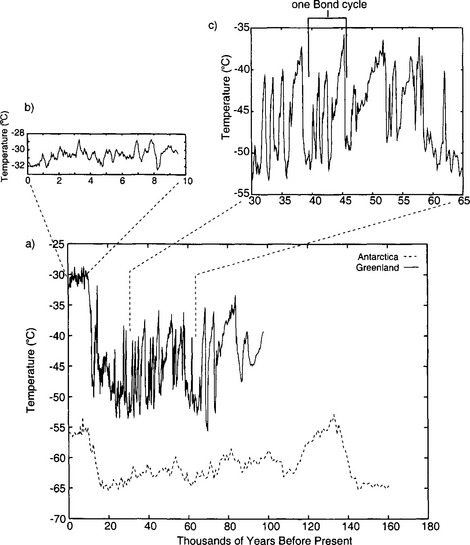
Fig. 18-9 (a) Temperature histories derived by borehole-temperature calibration of isotopic records, for Antarctica (Salamatin et al., 1998; Jouzel et al., 1993) and Greenland (Cuffey et al., 1995; Grootes et al., 1993). (b) A closer look at the Holocene. (c) A closer look at some of the rapid climate changes (D-O events) during the last glacial period. The magnitudes of these temperature swings are not yet calibrated, and may be only half as large as depicted here.
There is a striking contrast between the millennial variability of polar interglacial and glacial temperature histories. Whereas climate changes were frequent and large throughout the glacial period in both polar regions, the polar climate of the current interglacial (the Holocene) has been relatively stable (Dansgaard et al., 1993). The large, rapid millennial-scale climate change events during the glacial period are called Dansgaard–Oeschger (D–O) events in honor of their original discoverers. These many substantial climate changes within the last glacial period are definitively recorded as abrupt events in all ice cores from Greenland (Johnsen et al., 1997), and also appear in Antarctic cores in muted form (Bender et al., 1994). There are several lines of compelling evidence which argue that these isotopic changes are in fact temperature changes, and not simply changes in one of the other controls on δ: including the presence of gas isotopic spikes of appropriate magnitude, and coincident changes in CH4, accumulation rate, and atmospheric impurity deposition (see Sections 18.3.4,18.3.5.2, and 18.3.6).
The abrupt climate oscillations seen in the Greenland cores (D-O events) occurred in groups that outline a sawtooth pattern of initial abrupt warming followed by gradual cooling, each group lasting about 7 kyr (Bond et al., 1993). These are called Bond cycles(Figure 18-9). The D-O events within each Bond cycle show generally decreasing durations and maxima through time. Moreover, the Bond cycles are correlated to changes in sea-floor deposits, and in particular the cold extremes of the Bond cycles are coincident with massive iceberg discharge events from the North American ice sheet into the North Atlantic (Heinrich events; Broecker, 1994). This correlation, plus coincident changes in methane (see Section 18.3.5.2 below), plus the expression of these events in Antarctic cores and sea cores (e.g., Kennett and Ingram, 1995) show conclusively that these rapid environmental changes had global significance.
The most recent of these abrupt climate changes(11500 years ago; Fig. 18-9) was the termination of the Younger Dryas event, a 1000-year return to glacial conditions during the longer-term warming from glacial to interglacial (see Section 18.3.4). The termination of this cold climate was accomplished in a geologic instant – a mere 10 years. In this time, the temperature jumped by probably 5 to 10°C (Severinghaus et al., 1998) and the accumulation rate doubled. Earlier D–O events had many similarly abrupt transitions. Note, however, the lack of a prominent Younger Dryas event in the Antarctic.
The D-O events are far too rapid to be caused by insolation changes, and they most likely result from changes in ocean circulation. Their prominence and clarity in the Greenland cores relative to the Antarctic ones is due to the proximity of Greenland to the sites of deep-water formation in the North Atlantic and the tremendous amount of heat being delivered to them by the Gulf Stream (Broecker and Denton, 1989).
Though extremely stable compared to the glacial climate, the polar Holocene climate did vary. One notable rapid climate change event, a dip to lower temperature, occurred approximately 8 kyr ago (Alley et al., 1997). On average, the early Holocene was modestly warmer than the present. The past several thousand years have been cooler, especially during the 16th-19th centuries, a time known loosely as the Little Ice Age (LIA). There are direct records of this cold period from many places around the globe, and glaciers were substantially larger in mountain ranges of both hemispheres.
18.3.3 Deuterium Excess
Measurements of both the δ18O and the δD of precipitation over much of the globe reveal a very striking linear relationship between the two (an explanation is given in Box 2) called the Meteoric Water Line. The slope of this line is almost exactly dδD/dδ18 < O = 8 (Craig, 1961). If all isotopic fractionations in the water cycle occur during equilibrium processes, the intercept of this line would be approximately zero. Instead, the measured intercept is 8.6. This offset results from isotopic separation during evaporation from the ocean surface (Merlivat and Jouzel, 1979). Because this isotopic separation depends on evaporation rate it also depends on temperature, relative humidity and wind speed, all of which are interesting climatic parameters. Furthermore, the slope value of 8 also depends on air mass temperature early in its trajectory. For both of these reasons, measurements of deuterium excess (defined as d=δD – 8δ18O) along an ice core yield paleoclimate information (Jouzel et al., 1982; Johnsen et al., 1989), not about climate over the ice sheets but about climate of low to mid latitudes.
Analyses of d in modern snow (both its average value and its seasonal cycle) in Greenland and Antarctica show that the vapor source regions for the high-altitude interiors of the polar ice caps are located in the subtropics. Ice deposited in Antarctica during the last glacial period has average d lower by 4%o than the modern value, reflecting both colder ocean surface temperature and also higher relative humidity. In ice-age ice from Greenland, d varies from 4 to 8%o in anti-correlation with the temperature changes of the D-O events. This indicates a substantial northward shift of moisture sources during the warm phases of climate oscillations within the glacial period.
18.3.4 Accumulation Rates: Ancient Precipitation Gages
Accumulation rate is the net rate of mass addition to the ice-sheet surface (generally reported as thickness of ice per time), which equals the snowfall rate minus rate of loss by wind scour, sublimation and (at warm sites) melt. Snowfall rate is a climatic parameter of great interest, as it depends on atmospheric circulation and water content. Snowfall rate is approximately equal to accumulation rate at all but the driest of ice core sites.
To infer accumulation rate history from an ice core, one needs to measure the thickness of annual layers (either directly if annual layers are resolvable, or by differentiating the depth-age scale determined by other means) and then correct for the thinning of these layers caused by the ice flow(the vertical strain: Fig. 18-4). Estimates of vertical strain can be very uncertain for the deep part of an ice core. But vertical strain will not change rapidly with depth. Thus, if annual layers are resolvable one can learn relative accumulation rate changes across climate transitions with great confidence.
An alternative method for inferring accumulation rate relies on assuming that the rain of cosmogenic nuclides such as 10Be onto the ice sheet surface is known. Then high accumulation rate dilutes the cosmogenic nuclide so its concentration as measured in the ice core is inversely proportional to accumulation rate.
Accumulation rate histories from both Greenland and Antarctica all show substantially lower accumulation rates during glacial periods (Fig. 18-10), rates being as low as 25% of the modern value in central Greenland and 30% in East Antarctica. Much of this reduction is probably a consequence of thermodynamics; at saturation the content of water vapor in air is a strongly increasing function of temperature. During cold periods, the air masses over the ice sheets must be very dry. In central Greenland, accumulation rate inferences have annual resolution across the termination of the last glacial period, because annual layers are still readily distinguishable in ice of this age. At the end of the cold Younger Dryas period, accumulation rate doubled (Alley et al., 1993). Remarkably, this happened within a single decade. The earlier doubling of accumulation rate at 14 600 yr B.P. (before present) was similarly abrupt(Fig. 18-10).
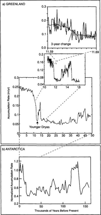
Fig. 18-10 (a) Accumulation rate history for Greenland (Alley et al., 1993; Cuffey and Clow, 1997), with insets focusing on the Younger Dryas cold interval and the very rapid termination of the last glaciation, with substantial change that occurred in only 3 years noted, derived from 10Be analysis. (after Alley et al., 1993). (b) Accumulation-rate history, normalized to the modern rate, for Antarctica (Raisbeck et al., 1987)
18.3.5 Trace Gases
18.3.5.1 Ice-core records of CO2
As explained in Section 18.3.1, the polar ice sheets trap and preserve air. Analyses (Sowers et al., 1997) of this air reveal the compositions of past atmospheres. One of the most important constituents that can be measured in ice samples is carbon dioxide (CO2). Excepting water vapor, a direct record of which is not preserved in polar ice, CO2 is the most important of Earth’s greenhouse gases, and past CO2 concentrations reveal significant variations in the global carbon cycle. The most reliable records of atmospheric CO2 are from Antarctic ice cores. Records from Greenland ice are not completely reliable due to high concentrations of carbonate dust in glacial-age ice there.
Ice-core records spanning the industrial revolution clearly show a large increase in CO2 levels over the last 200–250 years (Neftel et al., 1982; Etheridge et al., 1996). CO2 concentrations were approximately 275 ppmv (parts per million by volume) prior to 1750, and then began a steady rise to current levels of ∼360 ppmv. The most detailed ice-core record comes from Law Dome, a site in east Antarctica with a very high accumulation rate (∼1.2 m/yr) and accurate chronology(Fig. 18-11). Where this record overlaps the modern direct measurements of atmospheric CO2 agreement between the two records is excellent(Fig. 18-11).
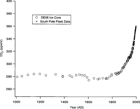
Fig. 18-11 Records of atmospheric CO2 in Antarctica for the past 1000 years. Plus signs are direct measurements of CO2 in air samples collected monthly at the South Pole (NOAA Climate Monitoring and Diagnostics Laboratory, Boulder, Colorado). Open circles are ice-core data from Law Dome, on the coast of east Antarctica (Etheridge et al., 1996).
Longer records show that atmospheric CO2 concentrations follow global climate trends (Barnola et al., 1987). Over the last two glacial-interglacial climate cycles, CO2 levels were approximately 280 ppmv during interglacial periods and substantially lower, approximately 190–210 ppmv, during the cold glacial(Fig. 18-12). A detailed record from the Byrd ice core illustrates the CO2 changes through the last glacial to interglacial transition(Fig. 18-13). CO2 levels began to rise about 18–20 kyr B.P. and reached interglacial levels by ∼ 10 000 kyr B.P.
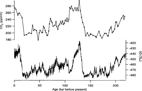
Fig. 18-12 Record of atmospheric CO2 over the past 220 000 years from the Vostok ice core (Jouzel et al., 1993; Barnola et al., 1987), and the corresponding deuterium isotope record temperature proxy (Jouzel et al., 1993) (see Section 18.3.2).
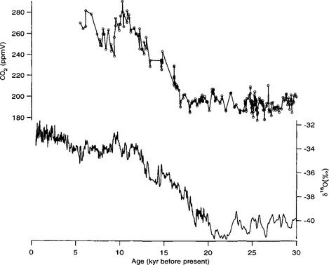
Fig. 18-13 High-resolution measurements of CO2 over the last glacial-interglacial transition from the Byrd ice core in west Antarctica (Neftel et al., 1982). Also plotted is the oxygen isotope record temperature proxy from the Byrd core (Johnsen et al., 1972). The time scale for the records plotted here is from Sowers and Bender (1995).
The nature and causes of the atmospheric CO2 concentration variations on different time scales are very interesting and only partially understood. The “anthropogenic transient” has been studied in detail. The period A.D. 1550–1800 was characterized by CO2 levels up to 6 ppm lower than the preceding 500 years (Fig. 18-11). The Little Ice Age (LIA) period of global cooling occurred during this time period, and cooler temperatures may have resulted in increased oceanic uptake of CO2 (due to the temperature dependence of its solubility), and enhanced wind-driven mixing of surface waters at high latitudes. Global cooling may also have influenced carbon uptake by terrestrial ecosystems. The rise in CO2 that began at about A.D. 1750 is believed to be due to a combination of land use changes (deforestation and other agricultural processes that release carbon to the atmosphere) and fossil fuel burning, with land use changes dominating prior to about A.D. 1900. Between A.D. 1000 and 1800, CO2 levels were between 275–284 ppmv(Fig. 18-11), and a value of 280 ppmv is often cited as the “pre-industrial” CO2 concentration. Records from the Byrd ice core show that during the entire Holocene period (0–10 000 years B.P.) CO2 levels actually varied between 245–280 ppm (Neftel et al., 1982) with a prominent minimum of 245–255 ppm at about 8000 years B.P.
The glacial-interglacial change in CO2 is about 80 ppm, and is not well understood. The shift occurred over about 8000 years during both the last and penultimate deglaciation. During the last deglaciation this rise in CO2 preceded sea-level rise and therefore the melting of ice sheets by 4 to 8 millennia (Sowers et al., 1993). During the penultimate deglaciation, the CO2 rise probably preceded sea-level rise by a few millennia (Broecker and Henderson, 1998). Both observations suggest an important role for CO2 in the warming during deglaciation and the CO2 change may have forced as much as 50% of the total glacial-interglacial warming (see Section 18.4.6 below).
Proposed explanations for glacial-interglacial CO2 change involve changes in ocean chemistry (see Chapter 10), either surface ocean total inorganic carbon (often abbreviated ΣCO2) levels or changes of the calcium carbonate budget of the ocean (Archer and Maier-Reimer, 1994; Broecker and Henderson, 1998). Much of the work on this subject has focused on the transition from low glacial CO2 levels to high interglacial CO2 levels, depicted in detail inFig. 18-12.
Changes in ΣCO2 could result from increases or decreases in the rate of organic carbon production in surface waters. Sinking organic material removes carbon from surface waters to the deep sea. Enhancement of this “biological pump” would decrease surface water PCO2 and draw down atmospheric CO2. If primary productivity (the rate at which plant organic matter is formed per unit area) during glacial times were higher than during interglacial times, atmospheric CO2 levels would have been lower due to this effect. One proposed mechanism for stimulating this additional productivity is enhanced phytoplankton growth due to higher fluxes of iron (a micronutrient) to the ocean surface in the dustier glacial atmosphere (Martin, 1990).
Mechanisms involving changes in the ocean’s calcium carbonate budget ( Chapter 10) invoke imbalances in the production, dissolution, and burial of calcium carbonate (the details of which are beyond the scope of this chapter) that can cause a rise or fall in atmospheric CO2. For example, if CaCO3 accumulation increased at the beginning of the glacial-interglacial transition, CO2 levels would rise, via the reaction . Possible reasons for changes in CaCO3 accumulation include growth or demise of coral reefs or shallow water carbonate sediments as sea-level rises or falls, changes in the ecology of marine plankton such that CaCO3 precipitating organisms are more or less abundant than other types of plankton, or changes in alkalinity of river waters. Because no proposed mechanisms appear to be fully supported by the paleoclimate record (Broecker and Henderson, 1998) the problem of adequately explaining the glacial-interglacial CO2 rise remains a major challenge.
18.3.5.2 Ice-core records of CH4
Methane (CH4), the Earth’s third most important greenhouse gas (behind water vapor and CO2) is produced almost exclusively by terrestrial sources (see Chapters 7 and 11). Natural methane sources include anaerobic microbial respiration in wetlands, termites, wild animals (ruminants), and a variety of other minor sources. Major anthropogenic sources are rice paddies, domestic cattle and other animals, and fossil fuel production. The primary methane sink is oxidation by OH in the troposphere, with a small fraction of the total methane production oxidized in soils and in the stratosphere ( Chapter 7).
Ice-core records covering the past three centuries (Etheridge et al., 1992; Blunier et al., 1993) show that methane concentration rose at the beginning of the industrial revolution, largely in parallel with increasing CO2 levels(Fig. 18-14). During the period from A.D. 900 to 1700, methane levels were between ∼675 and 725 ppbv, and started to rise sharply after about A.D. 1750 (Blunier et al., 1993). As this chapter is written, the global average value is 1730 ppbv (Dlugokencky et al., 1998). Levels are slightly lower in the southern hemisphere due to dominance of northern hemisphere sources. The ice-core values from the youngest section of the record shown inFig. 18-14 overlap, and agree well with, direct measurements at a site in Australia, supporting the fidelity of the ice core CH4 record. The growth rate of atmospheric methane increased from about 1 ppbv/yr in 1850 to 15 ppbv/yr in 1975 (Etheridge et al., 1992), with the exception of a period from 1920 to 1945 when the growth rate was stable. The general increase in growth rate during the industrial revolution presumably reflects the expansion of anthropogenic methane sources.
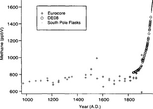
Fig. 18-14 Ice-core methane record for the past 1000 years. Plus signs are data from Eurocore in central Greenland (Blunier et al., 1993), and open circles are data from DE08, an ice core in East Antarctica (Etheridge et al., 1992). Dots are monthly atmospheric data from the South Pole (NOAA Climate Monitoring and Diagnostics Laboratory in Boulder, Colorado).
Longer ice-core records show that methane concentrations have varied on a variety of time scales over the past 220 000 years(Fig. 18-15) (Jouzel et al., 1993; Brook et al., 1996). Wetlands in tropical (30° S to 30° N) and boreal (50° N to 70° N) regions are the dominant natural methane source. As a result, ice-core records for preanthropogenic times have been interpreted as records of changes in methane emissions from wetlands. Studies of modern wetlands indicate that methane emissions are positively correlated with temperature, precipitation, and net ecosystem productivity (Schlesinger, 1996).
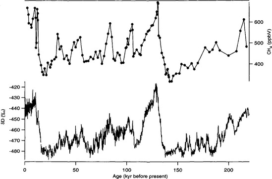
Fig. 18-15 Ice-core methane record from Vostok, Antarctica, for the past 220 000 years (Chappellaz et al., 1990; Jouzel et al., 1993).
Over the past 220 000 years methane concentrations ranged between 350 and 750 ppbv, compared to modern values in excess of 1700–1800 (Fig. 18-15). Over tens of millennia, methane variations appear to correspond to northern hemisphere insolation changes, correlate with Vostok paleotemperatures (Chappellaz et al., 1990) and have a strong 20 000 year periodicity, corresponding to the Earth’s precession cycle, which dominantly influences low-latitude climate. Changes in tropical monsoon strength have been proposed as a possible link; a more active monsoon and warmer temperatures could cause both greater wetland area and greater methane production in the tropics (Chappellaz et al., 1990). Recently, analysis of new 400 000+ year record from the Vostok site (Delmotte et al., 1998) suggests that a 40 000 year periodicity is also evident.
High-resolution methane records from Greenland (which in some cases resolve sub-century variation) considerably expand this picture of methane variability (Chappellaz et al., 1993; Brook et al., 1996). These records confirm the long-term patterns but also show higher-frequency millennial-scale variability closely associated with rapid temperature changes inferred from isotopic records; all of the interstadial events in the central Greenland δ18O record have correlated increases in atmospheric methane mixing ratio(Fig. 18-16). The methane response to rapid climate change during the last glacial period demonstrates that these rapid climate changes had widespread effects, because methane sources have a broad geographic distribution.
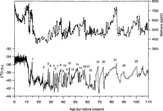
Fig. 18-16 Methane record for the past 110 000 years from the GISP2 ice core (Brook et al., 1996; Brook et al., in press). Numbers are labels for each of the warm “interstadial” periods within the cold glacial climate.
18.3.5.3 Ice-core records of N2O and other gases
Nitrous oxide (N2O) is a trace gas that contributes to the planetary greenhouse effect and to loss of stratospheric ozone ( Chapters 7 and 12). Ice-core data for N2O are considerably sparser than for CH4 and CO2. Machida et al. (1995) produced a high quality N2O record from a shallow Antarctic ice core (Fig. 18-17a) for the period A.D. 1750–1960. Their results show preanthropogenic levels of 273–280 ppbv, with an N2O minimum at about A.D. 1830, possibly coincident with the minimum in CO2. After about 1850, N2O levels rose, reaching values of 310 ppbv in the early 1990s. The preanthropogenic data from Machida et al. agree extremely well with similar measurements of N2O from South Pole firn air samples (Battle et al., 1996). The origin of the N2O rise during the anthropogenic period is not well understood. Possible sources include fertilizer, deforestation, combustion, and biomass burning.
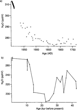
Fig. 18-17 Ice core records of N2O. (a) Data of Machida et al. (1995) from the H15 ice core, east Antarctica, for the time period 1750–1950, and monthly atmospheric N2O measurements at the South Pole from the NOAA Climate and Diagnostics Laboratory, Boulder, CO, for the period 1989–1998. (b) Data from Leuenberger and Siegenthaler (1992) from the Byrd ice core in West Antarctica.
Glacial-interglacial variations in N2O have been described by Leuenberger and Siegenthaler (1992) who showed that N2O levels during the glacial maximum at about 25 000 years B.P. were ∼ 190 ppbv (Fig. 18-17b). They found intermediate values of N2O (200–250 ppbv) between 30 000 and 40 000 years B.P.
Other trace gases important in atmospheric chemistry and climate (for example carbonyl sulfide and carbon monoxide) may also be measured in polar ice, and development of these and other measurements is underway in a number of laboratories around the world.
18.3.6 Non-Gaseous Impurities: Chemicals and Particles
In addition to the trace gases, many impurities, both soluble chemicals and insoluble particles, transfer from the atmosphere to the ice sheets and have measurable concentrations in ice cores. Such measurements are a window onto the history of atmospheric burdens and fluxes (from sources and to the ice sheets) for a great variety of aerosols (Delmas, 1992). These determine important radiative and chemical properties of the atmosphere, and are functions of atmospheric circulation intensity and the geography and strengths of sources and sinks. Inferring atmospheric loads and fluxes from concentrations in ice sheets is difficult and currently is plagued by important unsolved problems. A main difficulty is that we still do not have a quantitative understanding of the processes by which many species of atmospheric impurities are incorporated into ice.
Unlike the trace gases discussed in Section 18.3.5, most of the impurities discussed here have very short atmospheric residence times and are therefore not globally mixed. The records from Antarctica and Greenland therefore give unique information about the polar regions of each hemisphere.
Impurities travel from atmosphere to ice sheet surface either attached to snowflakes or as independent aerosols. These two modes are called wet and dry deposition, respectively. The simplest plausible model for impurity deposition describes the net flux of impurity to ice sheet (which is directly calculated from ice cores as the product of impurity concentration in the ice, Ci, and accumulation rate, ) as the sum of dry and wet deposition fluxes which are both linear functions of atmospheric impurity concentration Ca (Legrand, 1987):

where kd and kw are coefficients pertaining to dry and wet deposition, respectively. If an impurity deposits primarily by dry deposition, snowfall will act as a dilutant, so the ice-core concentration, Ci, will be inversely correlated to accumulation rate through time. If wet deposition predominates, Ci will be independent of accumulation rate and directly proportional to atmospheric concentration. In a general case, a plot of versus
 from ice-core data will, according to this simple model, yield a line whose slope and intercept are both proportional to ancient Ca and whose intercept indicates the importance of dry deposition. A change in Ca, across a climate transition is inferable from ratios of slopes and intercepts if the values kd and kw do not themselves change with climate. Herein lies the difficulty; this assumption is questionable and the model itself is a substantial simplification of reality for some species.
Most of the non-gaseous impurities in ice were once atmospheric aerosols. Atmospheric aerosols raining onto an ice sheet are of two types: primary aerosols, which are incorporated directly into the atmosphere as aerosols (these include continental dust and sea spray), and secondary aerosols which form in the atmosphere from gases. In addition to aerosol-derived impurities, some soluble gases in the atmosphere (HNO3 HCl, H2O2, and NH3) adsorb directly onto ice, and so are measured in a core as soluble ions rather than as constituents of trapped air bubbles. Some reactions occur during the aerosol phase which change the chemistry of primary aerosols. Primarily, secondary aerosol acids can react with salts in water droplets to separate the salts into metal ions and HCl gas. In modern Greenland and Antarctic snow, the secondary aerosol gas-derived acids dominate the chemistry, except very close to the coasts where sea salts can be important.
18.3.6.1 Sulfur cycle: and MSA
One of the most important of the acids is H2SO4, which (see Chapter 13 on the sulfur cycle) primarily results from dissolution of SO2 in water droplets. Both SO2 and the strong acid MSA are products of oxidation of DMS gas, which is emitted by organisms in the near-surface ocean. MSA is incorporated unaltered in the ice, so MSA measurements provide a relatively direct measure of DMS production and possible related albedo effects ( Chapter 13). (It does not provide a direct measure because H2SO4/MSA partitioning is not fixed.) The best measure of the relative contribution of biogenic gases to the total sulfur input is thought to be the MSA fraction (Whung et al., 1994), defined as the ratio MSA/(MSA+ ).
).
Histories of MSA and archived (Fig. 18-18) in the Greenland ice sheet (Saltzman et al., 1997) show that both atmospheric MSA concentrations and MSA fraction were lower during the cold glacial period than during the Holocene. The sulfur cycle-climate feedback was therefore probably a negative one in the North Atlantic, with increases in aerosol production accompanying, and opposing, climate warming from glacial to Holocene. However, MSA concentrations were low during the time of most rapid melt of the ice sheets (when presumably the ocean surface had relatively low salinity), and rose slowly throughout most of the Holocene, not peaking until approximately 3500 years ago. This slow response contrasts starkly with the rapid fluctuations of most climate parameters during deglaciation, and implies that the feedback is a delayed one. The most likely explanation for the slow response of the biogenic sulfur output, and for the glacial-interglacial contrast, is an ecological change, specifically a change in relative faunal abundances.
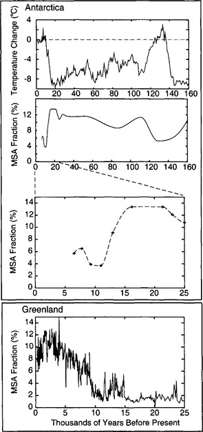
Fig. 18-18 Top two panels show the history of Antarctic MSA fraction (Legrand et al., 1991), and coincident isotopic temperature history (Jouzel et al., 1993). Bottom two panels present a closer look at the last 25 kyr, for both Antarctica and Greenland (Saltzman et al., 1997).
MSA and histories from Antarctica (Legrand et al., 1991) imply a very different response (Fig. 18-18) for the southern oceans than for those of the north. While
 not derived from seasalts was only modestly higher during glacial times (by less than a factor of two after accumulation correction), both MSA and MSA fraction were substantially higher during the coldest part of the last glacial period, approximately five times higher than Holocene values. Thus, in contrast to the North Atlantic, the southern oceans apparently yielded a substantial increase in biogenic sulfur flux during the glacial climate (and the associated climate feedback was positive). One possible explanation for this is that increased nutrient flux to the oceans via primary aerosols (see Section 18.3.5.1) fueled more biological activity.
Two further aspects of records deserve special mention. First, the recent and substantial anthropogenic production of SO2 has a clear signature in increased
 concentratons in Greenland accumulation, but not in northwestern Canada or the Antarctic (Mayewski et al., 1993). Second, large or local volcanic eruptions can produce substantial
 spikes.
18.3.6.2 Nitrogen cycle: and
and
The second important acid in polar snow is HNO3, which, along with other as well as NH3, can record nitrogen cycle perturbations. HNO3 and
 are products of NOx compound oxidation (see Chapter 12 on the nitrogen cycle), and
 is additionally a constituent of salts, such as Ca (NO3)2, which are primary aerosols. A major motivation for studying
 in ice cores is the role of its NOx precursors in controlling the oxidative capacity of the atmosphere. Both
 and
and are very interesting in that their histories do not correlate well with the vast majority of other ions and climate measures, especially in Greenland ice.
There are a wide variety of initial sources of for the ice sheets, including bacterial emissions, biomass burning, photochemical reactions, and lightning. These are generally low-mid-latitude continental sources. This very complicated mixed source renders interpretations of ice-core
 concentrations difficult. A further complication results from possible limitations on delivery of
 to ice-core sites by atmospheric circulation, due to the large distance from source regions to ice sheets coupled with limited residence times.
As with , anthropogenic activity has caused a modern increase in
 in Greenland firn (e.g., Mayewski et al., 1990). This appears to be the only unambiguous result from the many
 measurements. Atmospheric nitrate concentrations were approximately 20% lower over Greenland during glacial times than at present (Fuhrer and Legrand, 1997), which may reflect decreased nitrogen gas emissions from soils during the cold climate, but which may also reflect greater difficulty of transport resulting from the large ice sheets. In Antarctic ice, glacial-age nitrate concentrations are higher than in Holocene ice, and correlate strongly with primary aerosols from continental sources. Legrand et al. (1988) infer that much of this
 is from continental salts, and that the remainder, representing the gas-derived acid, had a lower concentration during the glacial than during the Holocene, as it did over Greenland.
Ammonium sources are biogenic and are also largely mid- or low-latitude continental. Main sources are emissions from soils and macro-biota, and fires. As with NO3, concentration depends importantly both on source strength and efficiency of transport from source to ice sheet. Atmospheric
 over Greenland was generally lower during the cold glacial climates, due to a combination of reduced source strength (resulting from colder and drier climate on the North American continent) and reduced transport of mid-latitude air into the Arctic (Meeker et al., 1997). But most of the
 variation is uncorrelated to the global climate, and in fact late Holocene
 concentrations are similar to those of the last glacial maximum. Greenland
 appears to be strongly correlated with summertime insolation in the northern hemisphere, except when the continental ice sheets were large, during which times
 was not delivered to the ice sheet efficiently.
18.3.6.3 Primary aerosols: seasalts and continental dust
The concentration of primary aerosols (Fig. 18-19) was substantially higher in the atmosphere of cold glacial climates than in that of warm interglacials (De Angelis et al., 1987; Mayewski et al., 1997). Many primary aerosols derive from seasalts (Na, Mg, Cl, K, and some Ca, SO4, NO3), whose entrainment in the atmosphere and deposition onto ice sheets increases strongly with increasing ocean surface wind speed and, less importantly, with decreasing sea-ice aerial cover. Other important primary aerosols are dust from the continents, especially insoluble particles (mostly aluminosilicates, for which Al is used as an index), but also CaCO3 and CaSO4, which are soluble. Entrainment and deposition of primary continental aerosol increases as a function of increased wind speed, increased aridity, and increased source area.
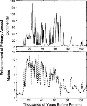
Fig. 18-19 Enhancement, relative to modern values, of marine and continental primary aerosols in Greenland through the last ice age (derived from Mayewski et al., 1997).
The markedly higher seasalt concentrations during glacial times are due to a combination of greater ocean surface wind strength in both hemispheres as well as stronger meridional transport (Herron and Langway, 1985). Estimates of the surface wind strength increase are 3 to 8 m/s. The markedly higher continental dust flux probably results from both increased wind strength and expansion of arid areas. Average dust grain size was larger during glacial times too, which indicates an increase in wind speed. The greater wind strength implied by these proxy records strongly suggests that the average equator-to-pole temperature gradients were larger during the cold climate. The isotopic signature of continental dust in both Greenland and Antarctica reveals the primary geographic source regions for ice age dust (Biscaye et al., 1997), which are central Asia and Patagonia, respectively. These areas must have been particularly dry then.
The increase in dust in the interior of Antarctica strongly implies that the flux of chemicals from continents to the southern oceans was also much higher during glacial times (Fig. 18-20). Because biological activity in vast areas of the southern oceans is limited by lack of nutrients (including iron) it is quite possible that this increase of dust flux stimulated marine biological activity where none exists during interglacials (the iron-fertilization hypothesis; see Section 18.3.5.1), which could contribute to reduction of atmospheric CO2. The temporal pattern of increases in continent-derived atmospheric dust is interesting in this context because of relative timing; it is clear from the ice-core records that dust flux increases occurred only well after temperature and greenhouse gas concentrations had begun to fall at the start of the last glacial period (De Angelis et al., 1987).
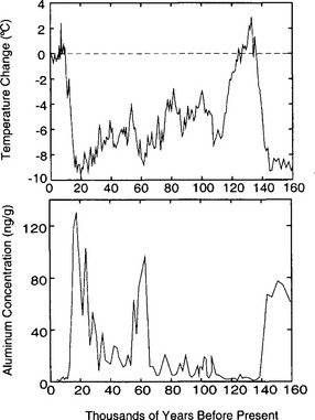
Fig. 18-20 Correlation of temperature history (Jouzel et al., 1993; Salamatin et al., 1998) and continent-derived dust reaching Antarctica (De Angelis et al., 1987).
Examples of inferred enhancements of atmospheric primary aerosol concentration in the glacial atmosphere relative to the modern are factors of 4 to 7 for insoluble particles from continents, and 3 for seasalts (Alley et al., 1995), over Greenland.
18.4 Some Lessons in Environmental History
18.4.1 Summary of the Ice-Age Experiment
Over the past two million years, changes of global average radiative energy input to the Earth have been regular but minor, while changes of seasonal energy input have been significant but asynchronous between north and south hemispheres. These insolation changes cause substantial global environmental changes, encompassing changes in atmospheric and oceanic composition and circulation, changes in the physical surfaces of continents, changes in the biosphere, and changes in associated chemical cycles. The transformation of a minor or geographically localized forcing into a major and global response is a direct consequence of both the strong coupling between diverse Earth systems and the operation of feedbacks.
The strong coupling of Earth systems is spectacularly evident in the ice-age cycles as nearly synchronous changes in temperature, precipitation, wind strength, ocean current strength, terrestrial and marine biota, continental ice volume, and atmospheric concentrations of greenhouse gases and aerosols. Many of these changes, or their direct consequences, are elegantly recorded in the 250 kyr environmental history retrieved from Vostok in the heart of the Antarctic ice sheet (Fig. 18-21), and in the history of the last major climate transition retrieved from central Greenland (Fig. 18-22).
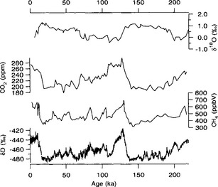
Fig. 18-21 The last 250 000 years of environmental history, recorded in the central Antarctic ice sheet. Bottom three panels are data from the Vostok ice core (Lorius et al., 1990; Jouzel et al., 1993). Top panel is marine data representing global ice volume (Shackleton et al., 1990).
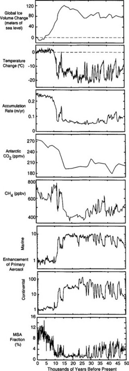
Fig. 18-22 The last 50 000 years of environmental history, recorded in central Greenland (GISP2 and GRIP ice cores), plus the CO2 record from Vostok, Antarctica, and global ice volume measured as sea level depression. (From top to bottom, references are: Shackleton, 1987; Cuffey et al., 1995 and Grootes et al., 1993; Cuffey and Clow, 1997; Chapellaz et al., 1990; Brook et al., 1996; Mayewski et al., 1997; Saltzman et al., 1997.)
In the global ice-age experiment, important positive feedbacks include long-term changes in continental-ice cover, sea-ice cover, greenhouse gas concentrations, oceanic heat transport, atmospheric aerosol load, and vegetation. Strongly positive rapid feedbacks are also operative. These most likely involve atmospheric water vapor and clouds, and seasonal snow cover, which together amplify temperature changes by a factor of two to four (see 18.4.6). Negative feedbacks are harder to identify, but probably involve poleward atmospheric heat transport, biogenic sulfur emissions in the northern hemisphere, and some aerosols. Many feedbacks that are not yet understood probably exist in addition to these, especially involving controls on biogeochemical cycling.
The Earth systems also act as a frequency modulator in the ice-age cycles. The dominant forcings of 20 and 40 kyr periodicity are directly expressed in environmental changes, but these are considerably over-shadowed by the 100 kyr periodicity of glacial-interglacial cycling, for which there is no significant forcing. This suggests that key elements of the Earth’s environmental systems have a long response time. Possible candidates are changes in the dynamic characteristics of the ice sheets themselves and the dependence of ice-sheet melt and calving rates on elevation changes caused by isostatic response of the Earth’s crust, which is rate-limited by creeping flow of the mantle (Peltier, 1987).
Another feature of the coupled Earth system exhibited in the ice-age experiment is that the global environment has modes, or relatively stable states that it maintains despite continual changes in external forcings. A manifestation is that extremes of climate have generally consistent values; the temperature minima attained during each of the past four glacial cycles are all very similar, as are each of the interglacial temperature maxima, despite the changing character of the insolation forcing. Climate modes likely reflect, in part, multiple stable configurations for ocean circulation. The consistency of extrema despite variable forcings, and the constancy of some climate periods despite continual changes in forcings (as during the Holocene) both indicate internal regulation of the Earth’s environmental systems. Self-regulation generally results from feedbacks (see Chapter 17).
18.4.2 Some Large and Abrupt Climate Changes
Despite gradual changes in forcings, some very large climate changes have occurred in very little time – on time scales that are short even compared to human lives and to cultural changes. The clearest example is the abrupt warming and increase in precipitation at the final termination of the last glacial period (the end of the Younger Dryas), which is recorded at high resolution in Greenland ice and shown by coincident methane changes and by southern hemisphere geologic records (Denton and Hendy, 1994) to involve a significant fraction of the globe. This particular change involved a sudden strengthening of the thermohaline circulation and consequent heat transport to the North Atlantic, and thus directly resulted from coupling of the oceans to other climate systems. A major question for research is whether such abrupt changes could be triggered by anthropogenic warming. There is at this point no reason to discount the possibility. Some modeling efforts (Stocker and Schmittner, 1997) have, for example, suggested that an increase in the freshwater flux to the North Atlantic from the continents could cause the thermohaline circulation to abruptly cease, plunging Europe into a cold climate unlike any in recent millennia.
18.4.3 Polar Amplification
A clear characteristic of global climate changes is their amplification in the polar regions. In glacial-interglacial cycling, temperature changes in the Arctic and Antarctic have been two to three times larger than the corresponding changes at low and mid-latitudes. This results, in part, from large albedo changes due to changing land and sea ice cover, and seasonal snowlines, and also from changes in ocean to atmosphere heat transfer as insulating sea-ice cover waxes and wanes. Polar amplification is very interesting because it implies the polar ice sheets (Greenland and West Antarctica) are particularly vulnerable to melt in a warmed climate, and because the melting of permafrost in tundra regions may release significant quantities of the powerful greenhouse gas CH4. The increase of global mean temperature over the past century has, however, been only modestly amplified over the North Atlantic, Scandinavia and Greenland (Overpeck et al., 1997), suggesting something is very different about the modern environment from past ones. Indeed there is now a substantial and negative anthropogenic radiative forcing at the mid-latitudes of the northern hemisphere, resulting from industry-generated particles and gases which form aerosols (see Chapter 7). Because these will change through time as technologies and economies change, it would be incorrect to view the modern Arctic as safe from amplified warming based on the past century.
18.4.4 Global Climate Sensitivity
One of the primary goals of “Earth systems” research is to learn how sensitive global climate is to changes in forcings, for instance how much temperature change results from a given increase in atmospheric CO2 content. A particular difficulty in learning the sensitivity to a given forcing is that the magnitude of climate change strongly depends on coincident changes in other forcings as a result of feedbacks and couplings. For the particular case of CO2, an initial increase in temperature due to CO2 change may increase atmospheric H2O and decrease polar albedo, both of which are strong climate forcings themselves. Subsequent changes in biogenic emissions and ocean circulation may be very important too. Thus the net sensitivity due to CO2 change is very difficult to quantify from physical models alone, due to the great complexity of system components and their couplings. Current models, for instance, do not attempt to predict changes in planetary albedo resulting from changes in marine biogenic emissions.
The information in paleoenvironmental records therefore is very valuable for better constraining sensitivities. The use of paleoenvironmental records is either through general circulation models (physical models of climate processes combined on a numerical imitation of our planet), or through robust but simplistic “state-variable” analyses.
18.4.5 General Circulation Models (GCMs)
Insofar as paleoenvironmental records reveal histories of both forcings and environments, the accuracy of GCMs may be tested by efforts to replicate these histories. Successful replication would suggest the models capture the essential behavior of the Earth and therefore have predictive ability. Further, GCM simulations of past climates may allow partitioning of net climate changes into components due to various forcings. GCM simulations of the ice-age Earth are very much works in progress.
Recent revisions to the boundary conditions (ice-sheet topography and sea surface temperatures) have added uncertainty to many of the GCM calculations of the past two decades. Moreover, all of these calculations use prescriptions for at least one central component of the climate system, generally oceanic heat transport and/or sea surface temperatures. This limits the predictive benefit of the models. Nonetheless, these models are the only appropriate way to integrate physical models of diverse aspects of the Earth systems into a unified climate prediction tool.
A consistent result from GCM simulations of ice-age climate is that the global cooling of 5 to 8°C can not result solely from the direct radiative forcings (Hansen et al., 1984; Webb et al., 1997) of insolation, greenhouse gas, ice cover and terrestrial albedo changes. To explain the ice ages, there must be a strong net feedback that magnifies temperature changes by a factor of 2 to 4. This feedback is most likely a combination of atmospheric water vapor and clouds. The global climate sensitivity implied by these models is at least 0.5°C/(W/m2), and plausibly greater than l°C/(W/m2).
18.4.6 State-Variable Analyses
An alternative approach to assessing climate sensitivity is to assume that some or all important elements of the Earth’s environmental systems are so strongly coupled (as one may infer fromFigs 18-21 and 18-22) that the behavior of the whole system may be represented by the behavior of a few variables, which are related using feedback factors or simple dynamic models. Though such analyses cannot substitute for process models operating on realistic geographic domains, they distill the essential lessons of environmental history without creating an illusory aura of physical completeness and accuracy.
Lorius et al. (1990) performed a simple multivariate analysis in which they correlate the temperature changes of the past 160 kyr (as recorded in the Vostok δD record) with changes in five forcings: atmospheric CO2 plus CH4, ice volume, aerosol loading (dust and separately), and insolation. These analyses establish that greenhouse gas variations correlate with temperature variations better than do any other forcings, and that these gas variations account for 40 to 60% of the climate change (and most likely 55 to 65%), in the correlative sense. This suggests that gas changes account for more than 2°C of the global deglacial warming. As the gas changes themselves can account directly for only 0.7°C, a feedback factor of greater than 3 is necessary (feedback factor being defined as the ratio of a temperature change to the temperature change due only to direct forcings).
A broader view was explored by Hoffert and Covey (1992), who used estimated forcings and geographically broad data from both the last glacial maximum and the mid Cretaceous to calculate two estimates of bulk climate sensitivity (change in temperature per change in radiative forcing) necessary to explain the paleotemperatures for these climates. Net forcings relative to the pre-industrial Holocene are –6.7 W/m2 and +15.7 W/m2 for the glacial and the Cretaceous, respectively, which yield sensitivities of 0.45°C/(W/m2) and 0.57°C/(W/m2). The recent revisions of last glacial maximum reconstructed temperatures (both low-latitude and polar) to lower values increases Hoffert and Covey’s LGM sensitivity to 0.9°C/(W/m2), and Lorius et al.’s feedback factor to 3.5 or 4. Regardless, all these sensitivities are comfortably within the range predicted for modern climate by GCMs. To infer a substantially lower sensitivity of Earth’s climate to forcings, one would have to invoke physically implausible large additional forcings for both Cretaceous and glacial periods. It is thus a reasonable suggestion (Hoffert and Covey, 1992) that these paleoclimate records preclude a low global sensitivity.
18.4.7 Perspective on Anthropogenic Forcings
Finally, paleoenvironmental records demonstrate conclusively that anthropogenic changes of CO2, CH4, SO4, NO3, and N2O are very large relative to their natural variability during the entire Holocene, and the modern polluted environment has no analog in at least the past 400 kyr. The magnitude of this human “experiment” is of the same magnitude as the natural experiment that buried the sites of Boston, Chicago, London and Stockholm beneath more than a kilometer of glacial ice, and produced the moraines and lakes that stimulated Agassiz’s revelations.
Agassiz, L. Etudes sur les glaciers. Amsterdam: Privately published; 1840.
Alley, R. B., Meese, D. A., Schuman, C. A., et al. Abrupt increase in Greenland snow accumulation at the end of the Younger Dryas event. Nature. 1993; 362:527–528.
Alley, R. B., Finkel, R. C., Nishiizumi, K., et al. Changes in continental and sea-salt atmospheric loadings in central Greenland during the most recent deglaciation: model-based estimates. J. Glaciol. 1995; 41:503–514.
Alley, R. B., Mayewski, P. A., Sowers, T., et al. Holocene climatic instability: a prominent, widespread event 8200 years ago. Geology. 1997; 25:483–486.
Archer, D., Maier-Reimer, E. Effect of deep sea sedimentary calcite preservation on atmospheric CO2 concentration. Nature. 1994; 367:260–264.
Barnola, J. M., Raynaud, D., Korotkevitch, Y. S., Lorius, C. Vostok ice core provides 160 000 year record of atmospheric CO2. Nature. 1987; 329:408–413.
Battle, M., Bender, M., Dowers, T., et al. Atmospheric gas concentrations over the past century measured in air from firn at the South Pole. Nature. 1996; 383:231–235.
Bender, M., Sowers, T., Dickson, M. -L., et al. Climate connections between Greenland and Antarctica during the last 100 000 years. Nature. 1994; 372:663–666.
Berner, R. A. Atmospheric carbon dioxide levels over Phanerozoic time. Science. 1990; 249:1382–1386.
Biscaye, P. E., Grousset, F. E., Revel, M., et al. Asian provenance of glacial dust (stage 2) in the Greenland Ice Sheet Project 2 ice core, Summit, Greenland. J. Geophys. Res. 1997; 102:26765–26781.
Blunier, T., Chappellaz, J. A., Schwander, J., et al. Atmospheric methane record from a Greenland ice core over the last 1000 years. Geophys. Res. Lett. 1993; 20:2219–2222.
Blunier, T., Chappellaz, J., Schwander, J., et al. Asynchrony of Antarctic and Greenland climate change during the last glacial period. Nature. 1998; 394:739–743.
Bond, G., Broecker, W., Johnsen, S., et al. Correlations between climate records from North Atlantic sediments and Greenland ice. Nature. 1993; 365:143–147.
Boyle, E. A. The role of vertical chemical fractionation in controlling late Quaternary atmospheric carbon dioxide. J. Geophys. Res. 1988; 93:701–715.
Broecker, W. S. Massive iceberg discharges as triggers for global climate change. Nature. 1994; 372:421–424.
Broecker, W. S., Denton, G. H. The role of ocean-atmosphere reorganizations in glacial cycles. Geochim. Cosmochim. Acta. 1989; 53:2465–2501.
Broecker, W. S., Henderson, G. M. The sequence of events surrounding Termination II and their implications for the cause of glacial-interglacial CO2 changes. Paleoceanography. 1998; 13:352–364.
Brook, E. J., Sowers, T., Orchardo, J. Rapid variations in atmospheric methane concentration during the past 110 000 years. Science. 1996; 273:1087–1091.
Brook, E. J., Harder, S., Severinghaus, J., and Bender, M. (in press). Atmospheric methane during the past 50 000 years: trends, interpolar gradient, and rate of change. In “AGU Monograph on Mechanisms of Millennial Scale Climate Change” (P. Clark, R. Webb, and L. Keigwin, eds). American Geophysical Union, Washington DC.
Cerling, T., Wang, Y., Quade, J. Expansion of C4 ecosystems as an indicator of global ecological change in the late Miocene. Nature. 1993; 361:344–345.
Chappellaz, J., Barnola, J. M., Raynaud, D., et al. Atmospheric methane record over the last climatic cycle revealed by the Vostok ice core. Nature. 1990; 345:127–131.
Chappellaz, J., Blunier, T., Raynaud, D., et al. Synchronous changes in atmospheric methane and Greenland climate between 40 and 8 kyr BP. Nature. 1993; 366:443–445.
CLIMAP Project members. The surface of the ice age Earth. Science. 1976; 191:1131–1137.
COHMAP Members. Climate changes of the last 18 000 years: Observations and model simulations. Science. 1988; 241:1043–1052.
Craig, H. Isotopic variations in meteoric waters. Science. 1961; 133:1702–1703.
Crowley, T. J., North, G. R. Paleoclimatology. Neuchatel: Oxford University Press; 1991.
Cuffey, K. M., Clow, G. D., Alley, R. B., et al. Large Arctic temperature change at the Wisconsin-Holocene glacial transition. Science. 1995; 270:455–458.
Cuffey, K. M., Clow, G. D. Temperature, accumulation and ice sheet elevation in central Greenland through the last deglacial transition. J. Geophys. Res. 1997; 102:26383–26396.
Curry, W. B., Duplessy, J. C., Labeyrie, L. D., Shackleton, N. J. Changes in the distribution of δ13C of deep water between the last glaciation and the Holocene. Paleoceanography. 1988; 3:317–341.
Dahe, Q., Petit, J. R., Jouzel, J., Stievenard, M. Distribution of stable isotopes in surface snow along the route of the 1990 International Trans-Antarctica Expedition. J. Glaciol. 1994; 40(134):107–118.
Dahl-Jensen, D., Johnsen, S. J. Paleotemperatures still exist in the Greenland ice sheet. Nature. 1986; 320:250–252.
Dansgaard, W. Stable isotopes in precipitation. Tellus. 1964; 16:436–468.
Dansgaard, W., Johnsen, S. J., Clausen, H. B., et al. Evidence for general instability of past climate from a 250-kyr ice-core record. Nature. 1993; 364:218–220.
De Angelis, M., Barkov, N. I., Petrov, V. N. Aerosol concentration over the last climatic cycle (160 kyr) from an Antarctic ice core. Nature. 1987; 235:318–321.
Delmas, R. J. Environmental information from ice cores. Rev. Geophys. 1992; 30:1–21.
Delmotte, M., Chappellaz, J., Raynaud, D., et al. Atmospheric methane changes during the last 400 kyr revealed by the Vostok ice core. EOS. 1998; 79:F151.
Denton, G. H., Bickheim, J., Wilson, S. C., Stuiver, M. Late Wisconsin and early Holocene glacial history, inner Ross Embayment, Antarctica. Quatern. Res. 1989; 31:151–182.
Denton, G. H., Hendy, C. H. Younger Dryas age advance of Franz Josef Glacier in the Southern Alps of New Zealand. Science. 1994; 264:1434–1437.
Dlugokencky, K., Masarie, A., Lang, P. M., Tans, P. P. Continuing decline in the growth rate of the atmospheric methane burden. Nature. 1998; 393:447–450.
Emiliani, C. Pleistocene temperatures. J. Geol. 1955; 63:538–578.
Etheridge, D. M., Pearman, G. I., Fraser, P. J. Changes in tropospheric methane between 1841 and 1978 from a high accumulation rate Antarctic ice core. Tellus. 1992; 44B:282–294.
Etheridge, D. M., Steele, L. P., Lagenfelds, R. L., et al. Natural and anthropogenic changes in atmospheric CO2 over the last 1000 years from air in Antarctic ice cores. J. Geophys. Res. 1996; 101:4115–4128.
Fuhrer, K., Legrand, M. Continental biogenic species in the Greenland Ice Core Project ice core: Tracing back the biomass history of the North American continent. J. Geophys. Res. 1997; 102(C12):26735–26745.
Grootes, P. M., Stuiver, M., White, J. W. C., et al. Comparison of oxygen isotope records from the GISP2 and GRIP Greenland ice cores. Nature. 1993; 366:552–554.
Guilderson, T. P., Fairbanks, R. G., Rubenstone, J. L. Tropical temperature variations since 20 000 years ago: modulating interhemispheric climate change. Science. 1994; 263:663–665.
Hammer, C. U., Clausen, H. B., Dansgaard, W., et al. Dating of Greenland ice cores by flow models, isotopes, volcanic debris, and continental dust. J. Glaciol. 1987; 20:3–26.
Hammer C., Mayewski P. A., Peel D., Stuiver M., eds. Greenland Summit ice cores. J. Geophys. Res.; 102. 1997:26317–26886.
Hansen, J., Lacis, A., Rind, D., et al, Climate sensitivity: analysis of feedback mechanisms. Geophys. Monogr. ; 20. Am. Geophys. Union, New York, 1984. 130–163.
Hartman, D. Global Physical Climatology. Washington DC: Academic Press; 1994.
Hays, J. D., Imbrie, J., Shackleton, N. J. Variations in the Earth’s orbit: Pacemaker of the ice ages. Science. 1976; 194:1121–1132.
Herron, M. M., Langway, C. C. Firn densification: An empirical model. J. Glaciol. 1980; 25:373–385.
Herron, M. M., Langway, C. C., Jr., Chloride, nitrate and sulfate in the Dye 3 and Camp Century Greenland ice coresLangway C. C., Jr., et al, eds. Greenland Ice Core: Geophysics, Geochemistry and the Environment. Geophys. Monogr. Series; 33. AGU, New York, 1985. 77–84.
Hoffert, M. I., Covey, C. Deriving global climate sensitivity from paleoclimate reconstructions. Nature. 1992; 360:573–576.
Horita, J., Wesolowski, D. J. Liquid-vapor fractionation of oxygen and hydrogen isotopes of water from the freezing to the critical temperature. Geochim. Cosmochim. Acta. 1994; 58(16):3425–3437.
Johnsen, S. J., Dansgaard, W., Clausen, H. B., Langway, C. C. Oxygen isotope profiles through the Antarctic and Greenland ice sheets. Nature. 1972; 235:429–434.
Johnsen, S. J., Dansgaard, W., White, J. W. C. The origin of Arctic precipitation under present and glacial conditions. Tellus. 1989; 41:452–469.
Johnsen, S. J., Clausen, H. B., Dansgaard, W., et al. The δ18O record along the Greenland Ice Core Project deep ice core and the problem of possible Eemian climatic instability. J. Geophys. Res. 1997; 102(C12):26397–26410.
Jouzel, J., Merlivat, L., Lorius, C. Deuterium excess in an East Antarctic ice core suggests higher relative humidity at the oceanic surface during the last glacial maximum. Nature. 1982; 299:688–691.
Jouzel, J., Merlivat, L. Deuterium and oxygen 18 in precipitation: modelling of the isotopic effects during snow formation. J. Geophys. Res. 1984; 89(D7):11749–11757.
Jouzel, J., Russell, G. L., Koster, R. D., et al. Simulations of the HDO and O atmospheric cycles using the NASA GISS general circulation model: the seasonal cycle for present-day conditions. J. Geophys. Res. 1987; 92(D12):14739–14760.
Jouzel, J., Barkov, N. I., Barnola, J. M., et al. Extending the Vostok ice-core record of paleoclimate to the penultimate glacial period. Nature. 1993; 364:407–412.
Jouzel, J., Waelbroeck, C., Malaize, B., et al. Climatic interpretation of the recently extended Vostok ice records. Clim. Dynam. 1996; 12:513–521.
Kennett, J. P., Ingram, B. L. A 20,000-year record of ocean circulation and climate change from the Santa Barbara Basin. Nature. 1995; 377:510–514.
Colloque C1 Legrand, M. Chemistry of Antarctic snow and ice. J. Physique. 1987; 48(3):77–86.
Legrand, M. R., Lorius, C., Barkov, N. I., Petrov, V. N. Vostok (Antarctica) ice core: atmospheric chemistry changes over the last climatic cycle (160 000 years). Atmos. Environ. 1988; 22(2):317–331.
Legrand, M., Feniet-Saigne, C., Saltzman, E. S., et al. Ice core record of oceanic emissions of dimethyl sulphide during the last climate cycle. Nature. 1991; 350:144–146.
Leuenberger, M., Siegenthaler, U. Ice-age concentration nitrous oxide from an Antarctic ice core. Nature. 1992; 360:449–451.
Lorius, C., Jouzel, J., Raynaud, D., et al. The ice-core record: climate sensitivity and future greenhouse warming. Nature. 1990; 347:139–145.
MacAyeal, D. R., Firestone, J., Waddington, E. Paleothermometry redux. J. Glaciol. 1993; 39(132):423–431.
Machida, T., Nakazawa, T., Fujji, Y., et al. Increase in atmospheric nitrous oxide concentration during the last 250 years. Geophys. Res. Lett. 1995; 22:2921–2924.
Majoube, M. Fractionnement en oxygene 18 et en deuterium entre l’eau et sa vapeur. J. Chim. Phys. 1971; 68:1423–1436.
Martin, J. H. Glacial-interglacial CO2 change: The iron hypothesis. Paleoceanography. 1990; 5:1–13.
Mayewski, P., Lyons, B., Spencer, M. J., et al. An ice core record of atmospheric response to anthropogenic sulphate and nitrate. Nature. 1990; 346:554–556.
Mayewski, P. A., Meeker, L. D., Twickler, M. S., et al. Ice core sulphate from three northern hemisphere sites: Source and temperature forcing implications. Atmos. Environ. A. 1993; 27(17/18):2915–2919.
Mayewski, P. A., et al. Major features and forcing of high-latitude northern hemisphere atmospheric circulation using a 110 000-year-long glaciochemical series. J. Geophys. Res. 1997; 102(C12):26345–26366.
Meeker, L. D., Mayewski, P. A., Twickler, M. S., et al. A 110 000-year history of change in continental biogenic emissions and related atmospheric circulation inferred from the Greenland Ice Sheet Project Ice Core. J. Geophys. Res. 1997; 102(C12):26489–26504.
Merlivat, L., Nief, G. Fractionnement isotopique lors des changements d’etats solide-vapeur et liquide-vapeur de l’eau a des temperatures inferieures a 0°C. Tellus. 1967; 19(1):122–127.
Merlivat, L., Jouzel, J. Global climatic interpretation of the deterium-oxygen 18 relationship for precipitation. J. Geophys. Res. 1979; 84:5029–5033.
Molnar, P., England, P. Late Cenezoic uplift of mountain ranges and global climate change: chicken or egg? Nature. 1990; 346:29–34.
Muller, R. A., MacDonald, G. J. Glacial cycles and astronomical forcing. Science. 1997; 277(5323):215–218.
Neftel, A., Oeschger, H., Schwander, J., et al. Ice core sample measurements give atmospheric CO2 content during the past 40 000 years. Nature. 1982; 295:220–223.
Overpeck, J., Hughen, K., Hardy, D., et al. Arctic environmental change of the last four centuries. Science. 1997; 278:1251–1256.
Paterson, W. S. B. The Physics of Glaciers, 3rd edn. Washington DC: Pergamon; 1994.
Peltier, W. R., Glacial isostasy, mantle viscosity and Pleistocene climatic changeRuddiman W. F., Wright H. E., Jr., eds. North America and Adjacent Oceans during the last deglaciation. The Geology of North America; Vol. K-3. Geological Society of America, Tarrytown, NY, 1987. 155–182.
Raisbeck, G. M., Yiou, F., Bourles, D., et al. Evidence for two intervals of enhanced 10Be deposition in Antarctic ice during the last glacial period. Nature. 1987; 326:273–277.
Raymo, M. E., Ruddiman, W. F., Backman, J., et al. Late Pliocene variation in northern hemisphere ice sheets and north Atlantic deep water circulation. Paleoceanography. 1989; 4:413–446.
Raymo, M. E., Ruddiman, W. F. Tectonic forcing of late Cenozoic climate. Nature. 1992; 359:117–122.
Reeh, N. Dating by ice flow modeling: a useful tool or an exercise in applied mathematics? In: Oeschger H., Langway C. C., eds. The Environmental Record in Glaciers and Ice Sheets. Boulder, CO: Wiley; 1989:141–159.
Ruddiman, W. F., Kutzbach, J. E. Plateau uplift and climatic change. Scient. Am. 1991; 264:66–75.
Salamatin, A. N., Lipenkov, V. Y., Barkov, N. I., et al. Ice core age dating and paleothermometer calibration based on isotope and temperature profiles from deep boreholes at Vostok Station (East Antarctica). J. Geophys. Res. 1998; 103(D8):8963–8977.
Saltzman, E. S., Whung, P. -Y., Mayewski, P. A. Methanesulfonate in the Greenland Ice Sheet Project 2 Ice Core. J. Geophys. Res. 1997; 102(C12):26649–26658.
Saltzman, B., Verbitsky, M. Late Pleistocene climatic trajectory in the phase space of global ice, ocean state, and CO2: Observations and theory. Paleoceanography. 1994; 9(6):767–779.
Schlesinger, W. H. Biogeochemistry: an analysis of global change. New York: Academic Press; 1996.
Severinghaus, J. P., Sowers, T., Brook, E. J., et al. Timing of abrupt climate change at the end of the Younger Dryas interval from thermally fractionated gases in polar ice. Nature. 1998; 391:141–146.
Shackleton, N. J. Oxygen isotope analyses and Pleistocene temperatures re-assessed. Nature. 1967; 215:15–17.
Shackleton, N. J. Oxygen isotopes, ice volume and sea level. Quatern. Sci. Rev. 1987; 6:183–190.
Shackleton, N. J., Berger, A., Peltier, W. R. An alternative astronomical calibration of the lower Pleistocene timescale based on ODP Site 677. Trans R. Soc. Edin. Earth Sci. 1990; 81:251–261.
Shuman, C. A., Alley, R. B., Anandakrishnan, S., et al. Temperature and accumulation at the Greenland Summit: Comparison of high-resolution isotope profiles and passive microwave brightness temperature trends. J. Geophys. Res. 1995; 100(D5):9165–9177.
Sowers, T., et al. A 135,000 year Vostok-SPEC-MAP common temporal framework. Paleoceanography. 1993; 8:737–766.
Sowers, T. A., Bender, M. Climate records during the last deglaciation. Science. 1995; 269:210–214.
Sowers, T., Brook, E. J., Etheridge, D., et al. An interlaboratory comparison of techniques for extracting and analyzing trapped gases in ice cores. J. Geophys. Res. 1997; 102:26527–26538.
Steig, E. J., Brook, E. J., White, J. W. C., et al. Synchronous climate changes in Antarctica and the North Atlantic. Science. 1998; 282:92–95.
Stocker, T. F., Schmittner, A. Influence of CO2 emission rates on the stability of the thermohaline circulation. Nature. 1997; 388(6645):862–865.
Stute, M., Schlosser, P., Clark, J. F., Broecker, W. S. Paleotemperatures in the southwestern United States derived from noble gases in groundwater. Science. 1992; 256:1000–1003.
Stute, M., Schlosser, P., Talma, A. S., et al. Uniform cooling of the low latitude continents during the last glacial maximum. EOS. 1995; 76:F296.
Thompson, L., et al. Late glacial stage and Holocene tropical ice core records from Huascaran, Peru. Science. 1995; 269:46–50.
Turekian, K. K. T. Global Environmental Change. Prentice Hall; 1996.
Webb, R. S., Rind, D. H., Lehman, S. J., et al. Influence of ocean heat transport on the climate of the Last Glacial Maximum. Nature. 1997; 385:695–699.
Whung, P. -Y., Saltzman, E. S., Spencer, M. J., et al. A two hundred year record of biogenic sulfur in a south Greenland ice core (20D). J. Geophys. Res. 1994; 97:6023–6036.